Theory of four-wave mixing and accompanying dissociation and population transfer controlled with laser-induced continuum structures

Abstract

A theory is developed and applied to the study of opportunities and specific features of coherent control of four-wave mixing as well as of the accompanying processes in the continuous-wave regime, which involve transitions between bound and free quantum states. Such opportunities become feasible through constructive and destructive interference of quantum pathways. Two coupling schemes of practical importance are investigated. In the first, a ladder energy level scheme, fully-resonant sum-frequency nonlinear-optical generation of short-wavelength radiation driven by several strong fields is investigated. The relaxation processes as well as absorption of the fundamental and generated radiations, which play an important role, are taken into consideration. It is shown that the generation output can be considerably increased through the appropriate adjustment of several laser-induced continuum structures. In the second, a folded scheme, a possible control of two-photon dissociation ($\Lambda$-scheme) using auxiliary laser radiation applied to the adjacent bound-free transition ($V$-configuration) is investigated. Besides dissociation, the proposed method enables one to control population transfer between two upper discreet levels via the lower-energy dissociation continuum, while direct transition between these states is not allowed. The opportunities of manipulating these processes as well as of four-wave-mixing-based spectroscopy are explored both analytically and through a numerical simulation for Na₂ dimers.

PACS: 42.50.Hz, 42.50.Ct,42.65.Ky, 42.65.Yj, 32.80.Fb., 32.80.Qk

Contents

1. Introduction 2

2. Four-wave mixing, absorption and refractive indices in ladder
      energy-level schemes controlled by interference of two LICS 4
      2.1. Equations for coupled electromagnetic waves and their solution 4
      2.2. Density matrix master equations and their solutions 5
      2.3. Laser-induced structures in absorption and refraction spectra
              at discrete and continuous transitions 9
      2.4. Resonance sum-frequency generation in strongly-absorbing media
              enhanced by quantum interference 12
      2.5. Absorption and dispersive spectra at Doppler-broadened transitions 17

3. Four-wave mixing, dissociation and population transfer controlled
      by LICS in folded energy-level schemes 19
      3.1. Quasistationary solution of density matrix equations 21
              3.1.1. Open configuration 24
              3.1.2. Closed configuration 25
      3.2. Numerical analysis 26
              3.2.1. Coherent control of populations and dissociation in folded schemes 27
              3.2.2. Coherent control of generated radiation in folded schemes 29

Conclusions 33

1 Introduction

The opportunities of laser control of optical properties and chemical reactivity of substances associated with the continuum energy states of atoms and molecules, and based on nonlinear quantum coherence and interference processes, have attracted considerable attention since their theoretical prediction GP2 , GP3 and experimental realization GP9 . These effects were shown to provide the feasibility of manipulating the spectral characteristics of the absorption, refraction, and nonlinear-optical conversion of weak radiations by an additional strong field, which is in resonance with a transition between an excited vacant level and a state in the continuum. The strong-field effects in such coupling configuration manifest themselves by the appearance of spectral autoionizing-like laser-induced continuum structures (LICS). In the presence of a real resonance autoionizing level a strong field has a strong influence on the spectral characteristics of this resonance too AI1 , AI2 , AI3 , Gel . The effects of the LICS on the absorption, refraction, nonlinear-optical generation and photoionization may differ significantly (see, for example, Refs Gel , Kn , Fau , 2a , 2c , Cav , 2d1 , bull , Kimb , 2e and the references therein). Most of the recent publications consider LICS in photoionization. The influence of real autoionizing levels and of the LICS on nonlinear susceptibility and four-wave mixing (FWM) has been investigated for frequencies of the other fields far from one-photon resonances 2c , Kimb . The interference of two LICS was shown to bring new qualitative effects in spectral properties of absorption, refraction and nonlinear optical generation of short-wavelength radiation Kimb .

Recently, the laser and chemical communities have focused on coherent quantum control of chemical reactions and other dissipation processes like photodissociation of molecules and photoionization of atoms TR1 , BrSh , TR2 , Br1 , D1 , Sh1 , D2 , U1 , U2 , 1D , 1DD , D4 , D3 , Br2 , R1 , Br3 , Br4 , Br5 , D5 , D8 , D9 , R2 , R3 , R4 , Gor1 , Sh2 , Sh3 , 102 , Mcool , R5 , R6 , R9 , Band , Br6 , R7 , R8 , 117 . In many cases, such control is based on implementation of the interference of different quantum channels, which give rise to laser-induced continuum structures (LICS) in the dissociation and ionization continua. Recent experiments aimed at control of photoionization of metastable helium atoms and some other processes making use of this technique are reported elsewhere Half , Yats , Berg .

This paper further develops theoretical approaches to these problems and reports novel opportunities for manipulating spectral characteristic of short-wavelength generation and photodissociation through the interplay of two LICS induced by strong continuous-wave laser fields coupling the dissociation continuum to two different bound states. Primary attention is paid to two important applications: (1) coherent control of sum-frequency short-wavelength generation in a ladder-type energy-level scheme (depicted in Fig. 1) and (2) coherent control of dissociation, population transfer and four-wave mixing feasible in a folded-type scheme (depicted in Fig. 9).

As concerns the first problem, we generalize our investigation of the LICS to the case of several strong control fields in situations when one can expect the strongest enhancement of the generated power. We consider the combined influence of the interference of two laser-induced structures in the continuum and of the laser-induced transparency (for the one-photon-resonant initial radiation and for the generated radiation) on the processes of nonlinear-optical generation of short-wavelength radiation. We demonstrate for the first time that nonlinear interference resonances in the output power of the radiation generated in an absorbing medium may differ considerably from the corresponding resonances in a transparent medium because of the combined influence of the nonlinear resonances in the nonlinear polarization and in absorption of both the initial and generated radiations.

A two-photon dissociation ($\Lambda$-scheme) controlled by an auxiliary laser field coupling continuum with another discrete state ($V$-configuration) is investigated for the second problem. All the coupled radiations are strong enough to drive molecular transitions. The proposed technique enables the coherent laser control of dissociation related to the lower laying molecular ’dark’ states that are not connected with the ground one by the allowed transition. On the other hand, the scheme under consideration enables one to transfer the population between two upper bound states which are not connected directly by the allowed transition. An analytical solution of the corresponding master density matrix equations of the problem is obtained, and a numerical analysis for relevant experimental conditions Half , Berg is performed. The possibility of manipulating the dissociation spectra and populations of excited states at the expense of the interference of quantum pathways through a variety of continuum states is explored. The dependence of the effects on the composed Fano parameters related to high excited levels, on the detuning between two LICS and on the intensities of the laser radiation is investigated.

2 Four-wave mixing, absorption and refractive indices in ladder energy-level schemes controlled by interference of two LICS

2.1 Equations for coupled electromagnetic waves and their solution

Let us consider four plane-polarized electromagnetic waves travelling along the $z$ axis of an isotropic medium,

$$E^{j}(z,t)={\rm Re}\{E_{j}(z)\exp[{\rm i}(\omega_{j}t-k_{j}z)]\},$$ (2.1)

where $k_{j}$ is the complex wave-number corresponding to the frequency $\omega_{j}$ ($j=1,2,3,S$). We assume that the fields $E_{1}$ and $E_{S}$ are weak compared to the driving fields $E_{2}$ and $E_{3}$, which do not vary along the medium. On the contrary, the fields $E_{1}$ and $E_{S}$ can change considerably along the medium, because of both absorption and nonlinear-optical conversion. Then the spacial behavior of the waves $E_{S}$ and $E_{1}$ is described by two coupled reduced wave equations,

$$dE_{S}(z)/dz ={\rm i}2\pi k_{S}^{\prime}\chi^{(3)}_{S}E_{2}E_{3}E_{1}(z)\exp({\rm i}\Delta kz),$$

$$dE_{1}(z)/dz ={\rm i}2\pi k_{1}^{\prime}\chi^{(3)}_{1}E^{*}_{2}E^{*}_{3}E_{S}(z)\exp(-{\rm i}\Delta kz).$$ (2.2)

Here $k_{j}=k_{j}^{\prime}-{\rm i}k_{j}^{\prime\prime}=(2\pi\omega_{j}/c)\chi_{j}$, $k_{j}^{\prime\prime}=\alpha_{j}/2$, and $\chi_{j},\alpha_{j}$ are the effective linear susceptibilities and absorption indices for the corresponding radiations, and $\chi^{(3)}_{1},\chi^{(3)}_{S}$ are the nonlinear susceptibilities describing the four-wave mixing processes: $\omega_{S}\leftrightarrow\omega_{1}+\omega_{2}+\omega_{3}$, $\Delta k=k_{S}-k_{1}-k_{2}-k_{3}$. The quantum conversion efficiency of the radiation $E_{1}$ into $E_{S}$ varies along the medium as

$$\eta_{{\rm q}}=(k_{1}^{\prime}/k_{S}^{\prime})|E_{S}(z)/E_{1}(0)|^{2}\exp(-\alpha_{S}z).$$ (2.3)

Let us first consider the case of low efficiency, for which the change in the $E_{1}$ caused by the nonlinear-optical conversion can be ignored. Then the second equation in (2.2) can be ignored as well and, with the account of the boundary condition $E_{S}(z=0)=0$, one obtains the following for the generated radiation and quantum conversion efficiency:

$$E_{S}(z)=(2\pi k_{S}^{\prime}/\Delta k)\chi_{S}^{(3)}E_{1}E_{2}E_{3}[\exp(-{\rm i}\Delta kz)-1],$$ (2.4)

$$\eta_{\rm q}(z)={k_{S}^{\prime}}{k_{1}}^{\prime}(\big{|}2\pi\chi_{S}^{(3)}E_{2}E_{3}\big{|}^{2}/|\Delta k|^{2})\exp(-\alpha_{S}z)\big{|}\exp(-{\rm i}\Delta kz)-1\big{|}^{2}.$$ (2.5)

If the medium length is much shorter than the minimum absorption length $L_{abs}=\min\{L_{1}=2/\alpha_{1},L_{S}=2/\alpha_{S}\}$ and both of these are assumed much shorter than the coherence length $L_{coh}=\Delta k^{\prime-1}$, then Eq. (2.5) reduces to the approximate formula

$$\eta_{{\rm q}}={k_{S}}^{\prime}{k_{1}}^{\prime}\big{|}2\pi\chi_{S}^{(3)}E_{2}E_{3}\big{|}^{2}L_{\rm e}^{2},$$ (2.6)

where $L_{\rm e}$ represents either the length of the medium (in the case of weak absorption) or the optimal length of the order of $\min\{L_{abs},L_{coh}\}$.

For a medium with substantial absorption dispersion ($\alpha_{1}\neq\alpha_{S}$), but $\Delta k^{\prime}=0$ and $\chi^{(3)}_{1}=\chi^{(3)*}_{S}$, the solution of equations (2.2), for the more general case of considerable conversion, takes the form tim

$$\eta_{\rm q}(z)=4\frac{\tilde{\eta}_{{\rm q}0}}{|b|}\exp\left[-(\alpha_{1}+\alpha_{S})\frac{z}{2}\right]\left[{\rm sinh}^{2}\left(\sqrt{\frac{(|b|-b)}{2}}\frac{z}{2}\right)+\sin^{2}\left(\sqrt{\frac{(\mid b\mid+b)}{2}}\frac{z}{2}\right)\right].$$ (2.7)

Here $\tilde{\eta}_{q0}=k_{1}^{\prime}k_{S}^{\prime}\mid 2\pi\chi^{(3)}_{S}E_{2}E_{3}\mid^{2}$ is the conversion efficiency per unit of the medium length under constant fundamental radiations, and $b=4\tilde{\eta}_{q0}-(\alpha_{1}-\alpha_{S})^{2}/4$ defines the difference between the rates of absorption and nonlinear-optical conversion of the radiations. If $b<0$, the conversion rate of $\hbar\omega_{1}$ photons into $\hbar\omega_{S}$ photons is less than their absorption rate; if $b=0$, the photon absorption and conversion rates are equal; and if $b>0$, the nonlinear-optical conversion rate exceeds the absorption rate. In the latter case, one can expect an oscillatory dependence of the transfer of the weak radiations from one to the another and back along the medium.

The susceptibilities $\chi^{(3)}_{S}$, $\chi^{(3)}_{1}$, $\chi_{S}$ and $\chi_{1}$ can be derived from the medium polarizations at the corresponding frequencies:

$$P(\omega_{j})=\chi_{j}E_{j},\quad P^{\rm NL}(\omega_{S})=\chi^{(3)}_{S}E_{1}E_{2}E_{3},\quad P^{\rm NL}(\omega_{1})=\chi^{(3)}_{1}E_{S}E^{*}_{2}E^{*}_{3}.$$ (2.8)

These components can be calculated conveniently with the aid of a density matrix, $\rho_{ij}$, as

$$\mathcal{P}(\omega_{j})=N\rho_{ij}(\omega_{j})d_{ji}+{\rm c.c.},$$ (2.9)

where $N$ is the atomic number density in the medium, and ${d}_{ji}$ is a matrix element of the projection of the transition electric-dipole moment along the direction of the electric vector of the corresponding field. The problem of finding and optimizing the quantum efficiency of the conversion process thus reduces to finding the off-diagonal elements of the density matrix.

2.2 Density matrix master equations and their solutions

First, we shall consider the transition scheme depicted in Fig. 1. A strong field ${\mathit{E}}_{2}$ at frequency $\omega_{2}$ is close to resonance with the transition between levels $m$ and $n$, while the strong fields ${\mathit{E}}$ and ${\mathit{E}}_{3}$ at frequencies $\omega$ and $\omega_{3}$ are in resonance with the transitions between levels $f$ and $n$ and some states in the continuum. Radiation at the frequency $\omega_{S}$ can be either a probe or generated by four-wave mixing. We shall investigate the influence of the strong fields on the spectral characteristics of the absorption of the radiations ${\mathit{E}}_{1}$ and ${\mathit{E}}_{S}$ at the frequencies $\omega_{1}$ and $\omega_{S}$ (both as independent probe radiations or, alternatively, as the frequencies linked through generation, $\omega_{S}=\omega_{1}+\omega_{2}+\omega_{3}$). The field $E_{1}$ is assumed close to resonance with the transition from the ground state to the level $m$ and $E_{S}$ to the transition from the ground state to the continuum. These radiations are weak, so that a change in the level populations due to all resonant couplings can be ignored. We neglect the degeneration of all states, including those in the continuum. In addition to the contribution of the off-resonant continuum states, we account for the contribution of discrete off-resonant levels which are combined to form the level $k$ in Fig. 1. We suppose that the detunings $\mid\omega_{1}$-$\omega_{gm}\mid$, $\mid\omega_{1}+\omega_{2}-\omega_{gn}\mid$ and $\mid\omega-\omega_{3}-\omega_{nf}\mid$ are considerably less than all the other detunings.

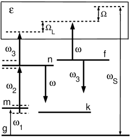
Figure 1: LICS-based coherent control in ladder schemes.

The equations for the density matrix, considered in the interaction representation to within the first order of perturbation theory in weak fields, can be written as follows:

$$d\rho_{gm}/dt+\Gamma_{gm}\rho_{gm}={\rm i}(\rho_{gg}V_{gm}+\rho_{gn}V_{nm}),$$

$$d\rho_{gn}/dt+\Gamma_{gn}\rho_{gn}={\rm i}\int\rho_{g\varepsilon}V_{\varepsilon n}d\varepsilon+{\rm i}\rho_{gm}V_{mn}+{\rm i}\sum\rho_{gk}V_{kn},$$

$$d\rho_{gf}/dt+\Gamma_{gf}\rho_{gf}={\rm i}\int\rho_{g\varepsilon}V_{\varepsilon f}d\varepsilon+{\rm i}\sum\rho_{gk}V_{kf},$$ (2.10)

$$d\rho_{g\varepsilon}/dt={\rm i}(\rho_{gg}V_{g\varepsilon}\hbox{{+}}\rho_{gn}V_{n\varepsilon}\hbox{{+}}\rho_{gf}V_{f\varepsilon}),$$

$$d\rho_{gk}/dt+\Gamma_{gk}\rho_{gk}={\rm i}(\rho_{gn}V_{nk}+\rho_{gf}V_{fk}).$$

Here, the index $\varepsilon$ denotes the continuum states; $V_{mn}=G_{mn}\exp[{\rm i}(\omega_{2}-\omega_{nm})t],V_{g\varepsilon}=G_{g\varepsilon}\exp[{\rm i}(\omega_{S}-\omega_{g\varepsilon})t],V_{n\varepsilon}=G_{n\varepsilon}\exp[{\rm i}(\omega_{3}-\omega_{n\varepsilon})t],V_{gm}=G_{gm}\exp[{\rm i}(\omega_{1}-\omega_{gm})t],V_{f\varepsilon}=G_{f\varepsilon}\exp[{\rm i}(\omega-\omega_{f\varepsilon})t],V_{kn}=G_{kn}\exp[{\rm i}(\omega-\omega_{kn})t],V_{kf}=G_{kf}\exp[{\rm i}(\omega_{3}-\omega_{kf})t]$ are the matrix elements of the Hermitian interaction Hamiltoman $\hat{V}$, considered in the electric-dipole approximation and in the interaction representation (in units of $\hbar$); $V_{ij}$ = $V^{*}_{ji};G_{mn}=-{E}_{2}{d}_{mn}/2\hbar,G_{g\varepsilon}=-{E}_{4}{d}_{g\varepsilon}/2\hbar,$ etc.; and $\Gamma_{ij}$ is the homogeneous half-width of the $i-j$ transition. In the approximation of the weak fields $E_{1}$ and $E_{S}$, we obtain $\rho_{gg}\approx 1,\rho_{m}\approx\rho_{n}\approx\rho_{f}<<1.$

Under steady-state conditions, each off-diagonal element of the density matrix is a sum of two components, which may oscillate at different frequencies:

$$\rho_{g\varepsilon} =r_{g\varepsilon}\exp[{\rm i}(\omega_{S}-\omega_{g\varepsilon})t]+R_{g\varepsilon}\exp[{\rm i}(\omega_{1}+\omega_{2}+\omega_{3}-\omega_{g\varepsilon})t],$$

$$\rho_{gn} =r_{gn}\exp[{\rm i}(\omega_{S}-\omega_{3}-\omega_{gn})t]+R_{gn}\exp[{\rm i}(\omega_{1}+\omega_{2}-\omega_{gn})t],$$

$$\rho_{gm} =r_{gm}\exp[{\rm i}(\omega_{S}-\omega_{3}-\omega_{2}-\omega_{gm})t]+R_{gm}\exp[{\rm i}(\omega_{1}-\omega_{gm})t],$$ (2.11)

$$\rho_{gf} =r_{gf}\exp[{\rm i}(\omega_{S}-\omega-\omega_{gf})t]+R_{gf}\exp[{\rm i}(\omega_{1}+\omega_{2}+\omega_{3}-\omega-\omega_{gf})t],$$

$$\rho_{gk} =r_{gk}\exp[{\rm i}(\omega_{S}-\omega_{3}-\omega-\omega_{gk})t]+R_{gk}\exp[{\rm i}(\omega_{1}+\omega_{2}-\omega-\omega_{gk})t].$$

By substituting (2.11) into (2.10), one can see that the set of differential equations under consideration reduces to two independent sets of algebraic equations, where each refers to the processes determined by only one weak field:

$${\rm i}R_{gm}D_{gm}=-G_{gm}-R_{gn}G_{nm},\qquad D_{gm}=\Gamma_{gm}+{\rm i}(\omega_{1}-\omega_{gm}),$$

$${\rm i}R_{gn}D_{gn}=-\int R_{g\varepsilon}G_{\varepsilon n}d\varepsilon-R_{gm}G_{mn}-R_{gk}G_{kn},\/D_{gn}=\Gamma_{gn}+{\rm i}(\omega_{1}+\omega_{2}-\omega_{gn}),$$

$${\rm i}R_{g\varepsilon}D_{g\varepsilon}=-R_{gn}G_{n\varepsilon}-R_{gf}G_{f\varepsilon},\qquad D_{g\varepsilon}={\rm i}(\omega_{1}+\omega_{2}+\omega_{3}-\omega_{g\varepsilon}),$$ (2.12)

$${\rm i}R_{gf}D_{gf}=-\int R_{g\varepsilon}G_{\varepsilon f}d\varepsilon-R_{gk}G_{kf},\qquad D_{gf}=\Gamma_{gf}+{\rm i}(\omega_{1}+\omega_{2}+\omega_{3}-\omega-\omega_{gf}),$$

$${\rm i}R_{gk}D_{gk}=-(R_{gn}G_{nk}-R_{gf}G_{fk}),\qquad D_{gk}=\Gamma_{gk}+{\rm i}(\omega_{1}+\omega_{2}-\omega-\omega_{gk}),$$

$${\rm i}r_{g\varepsilon}p_{g\varepsilon}=-G_{g\varepsilon}-r_{gn}G_{n\varepsilon}-r_{gf}G_{f\varepsilon},\qquad p_{g\varepsilon}={\rm i}(\omega_{S}-\omega_{g\varepsilon}),$$

$${\rm i}r_{gn}p_{gn}=-\int r_{g\varepsilon}G_{\varepsilon n}d\varepsilon-r_{gm}G_{mn}-r_{gk}G_{kn},\/p_{gn}=\Gamma_{gn}+{\rm i}(\omega_{S}-\omega_{3}-\omega_{gn}),$$

$${\rm i}r_{gm}p_{gm}=-r_{gn}G_{nm},\qquad p_{gm}=\Gamma_{gm}+{\rm i}(\omega_{S}-\omega_{3}-\omega_{2}-\omega_{gm}),$$ (2.13)

$${\rm i}r_{gf}p_{gf}=-\int r_{g\varepsilon}G_{\varepsilon f}d\varepsilon-r_{gk}G_{kf},\qquad p_{gf}=\Gamma_{gf}+{\rm i}(\omega_{S}-\omega-\omega_{gf}),$$

$${\rm i}r_{gk}p_{gk}=-r_{gn}G_{nk}-r_{gf}G_{fk},\qquad p_{gk}=\Gamma_{gk}+{\rm i}(\omega_{S}-\omega_{3}-\omega-\omega_{gk}).$$

Here and later the repeated index $k$ indicates summation over all discrete off-resonant levels combined to form the level $k$.

Equations (2.12) describe the absorption of ${E}_{1}$ and generation at the frequency $\omega_{S}$, whereas (2.13) presents the absorption of ${E}_{S}$ and parametric conversion of $E_{S}$ back into $E_{1}$. One can solve (12) by substituting the third equation into the second and fourth. Then, in the calculation of the integrals, one can employ the $\zeta$-function,

$$[-{\rm i}(\omega_{S}-\omega_{\varepsilon g})]^{-1}=\pi\delta(\omega_{S}-\omega_{\varepsilon g})+{\rm i}{\cal P}(\omega_{S}-\omega_{\varepsilon g})^{-1},$$ (2.14)

where $\delta(\xi)$ is the delta function, and $\cal P$ is the principal value obtained by integration. This leads to the following equations:

$$R_{g\varepsilon}={\rm i}[G_{n\varepsilon}-G_{f\varepsilon}(\gamma_{nf}/\gamma_{ff})\beta_{f}(1-{\rm i}q_{nf})/X_{f}]R_{gn}/D_{g\varepsilon},$$

$$R_{gm}={\rm i}\frac{G_{gm}+R_{gn}G_{nm}}{X_{m}\Gamma_{gm}},\>R_{gn}=-\frac{G_{gm}G_{mn}X_{f}}{\Gamma_{gf}\Gamma_{gn}X_{m}(1+g_{nn})(X_{n}X_{f}-K+A_{m}X_{f})},$$ (2.15)

where

$$\beta_{f} =g_{ff}/(1+g_{ff}),\quad\beta_{n}=g_{nn}/(1+g_{nn}),\quad g_{nn}=\gamma_{nn}/\Gamma_{gn},\quad g_{ff}=\gamma_{ff}/\Gamma_{gf},$$

$$K =\beta_{f}\beta_{n}(1-{\rm i}q_{nf})^{2},\quad A_{m}=g_{mn}/X_{m}(1+g_{nn}),\quad g_{mn}=|G_{mn}|^{2}/\Gamma_{gm}\Gamma_{gn};$$

$$q_{ij} =\delta_{ij}/\gamma_{ij},\>\gamma_{ij}=\pi\hbar G_{i\varepsilon}G_{\varepsilon j}\mid_{\varepsilon=\hbar\omega_{S}}+{\rm Re}(G_{ik}G_{kj}/p_{gk}),$$

$$\delta_{ij} =\hbar P\int d\varepsilon\frac{G_{i\varepsilon}G_{\varepsilon j}}{(\hbar\omega_{S}-\varepsilon)}+{\rm Im}[G_{ik}G_{kj}/p_{gk}],$$

$$X_{i} =1+{\rm i}x_{i},\>x_{n}=(\Omega_{1}+\Omega_{2}-\delta_{nn})/(\Gamma_{gn}+\gamma_{nn}),\>x_{m}=\Omega_{1}/\Gamma_{gm},$$

$$x_{f} =(\Omega_{1}+\Omega_{2}-\Omega_{L}-\delta_{ff})/(\Gamma_{gf}+\gamma_{ff})=(\omega_{1}+\omega_{2}+\omega_{3}-\omega-\omega_{gf}-\delta_{ff})/(\Gamma_{gf}+\gamma_{ff}),$$

$$\Omega_{L} =(\omega+\omega_{gf})-(\omega_{3}+\omega_{gn}),\>\Omega_{1}=\omega_{1}-\omega_{gm},\quad\Omega_{2}=\omega_{2}-\omega_{mn}.$$ (2.16)

Here $\Omega_{L}$ is the spacing between the quasi-levels induced by the radiations $E$ and $E_{3}$ in the continuum. The Fano parameters $q_{ij}$ fano are assumed real and indicate the ratio of the light-induced shifts and the broadening of the corresponding resonances by the control fields. In the adopted approximation, these parameters are independent of the field intensities and are governed solely by the properties of the investigated atom.

Following the same procedure as above and bearing in mind the condition $\omega_{S}=\omega_{1}+\omega_{2}+\omega_{3}$, one finds from the set of equations (2.13) that

$$r_{g\varepsilon} ={\rm i}\{G_{g\varepsilon}-G_{f\varepsilon}(\gamma_{gf}/\gamma_{ff})\beta_{f}(1-{\rm i}q_{gf})/X_{f}+r_{gn}[G_{n\varepsilon}-G_{f\varepsilon}(\gamma_{nf}/\gamma_{ff})\beta_{f}(1-{\rm i}q_{nf})/X_{f}]\}/p_{g\varepsilon},$$

$$r_{gm} ={\rm i}\frac{r_{gn}G_{nm}}{X_{m}\Gamma_{gm}},\>r_{gn}=\frac{(1-{\rm i}q_{fn})(1-{\rm i}q_{gf})\gamma_{gf}\gamma_{fn}/(\Gamma_{gf}+\gamma_{ff})-(1-{\rm i}q_{gn})X_{f}\gamma_{gn}}{(1+g_{nn})\Gamma_{gn}(X_{f}X_{n}-K+A_{m}X_{f})}.$$ (2.17)

The calculation of $R_{gm}$ from (2.15) and $r_{g\varepsilon}$ from (2.17), and application of formulas (2.8) and (2.9) after integration over the continuum states, gives the following expressions for the absorption and refractive indices at the frequencies $\omega_{1}$ and $\omega_{S}$, respectively:

$$\dfrac{\alpha(\omega_{1})}{\alpha_{10}} ={\rm Re}F_{1},\>\dfrac{n(\omega_{1})-1}{2(n_{1\max}-1)}={\rm Im}F_{1},$$

$$F_{1} =\dfrac{1}{X_{m}}{\biggl{[}}1-\dfrac{A_{m}X_{f}}{X_{n}X_{f}+A_{m}X_{f}-K}{\biggr{]}},$$ (2.18)

$$\dfrac{\alpha(\omega_{S})}{\alpha_{S0}} ={\rm Re}F_{S},\>\dfrac{n(\omega_{S})-1}{2(n_{S\max}-1)}={\rm Im}F_{S},$$

$$F_{S} =\biggl{[}1-\dfrac{X_{f}X_{n}(A_{n}+A_{f})-U+A_{m}A_{f}X_{f}}{{X_{f}X_{n}-K+A_{m}X_{f}}}\biggr{]}$$

$$=\biggl{[}1-A_{f}-A_{n}-\dfrac{K(A_{n}+A_{f})-U-A_{m}A_{n}X_{f}}{X_{f}X_{n}-K+A_{m}X_{f}}\biggr{]}$$

$$=\biggl{[}1-A_{f}-\widetilde{A}_{n}-\dfrac{K(\widetilde{A}_{n}+A_{f})-U}{X_{f}\widetilde{X}_{n}-K}\biggr{]}.$$ (2.19)

Here $\alpha_{10}$ is the absorption index with the fields intensities and detunings turned to zero, and $\alpha_{S0}$ is the similar quantity for a transition to the continuum; $n_{1\max}$ and $n_{S\max}$ are the maximum values of the corresponding refractive indices under control fields turned off; and

$$A_{f}=\beta_{f}{(1-{\rm i}q_{gf})^{2}/X_{f}};\>A_{n}=\beta_{n}{(1-{\rm i}q_{gn})^{2}/X_{n}};\>U=2\beta_{f}\beta_{n}(1-{\rm i}q_{gf})(1-{\rm i}q_{fn})(1-{\rm i}q_{ng}).$$

The functions $\widetilde{A}_{n}=\beta_{n}(1-{\rm i}q_{gn})^{2}/\widetilde{X}_{n}$ and $\widetilde{X}_{n}=X_{n}+A_{m}$ account for the perturbation of a two-photon resonance with the level $n$ by the strong fields. The expressions for the refractive index are obtained on the assumption that this index is close to unity in the absence of the fields.

The calculation of $R_{g\varepsilon}$ and $r_{gm}$ from the expressions (2.15) and (2.17), which is carried out making use of formulas (2.8) and (2.9) and integration over the states in the continuum, gives expressions for the FWM nonlinear susceptibility at $\omega_{S}=\omega_{1}+\omega_{2}+\omega_{3}$ as

$$\frac{\chi^{(3)}(\omega_{S})}{\chi_{S0}^{(3)}}=\frac{X_{f}-\beta_{f}(1-{\rm i}q_{nf})(1-{\rm i}q_{fg})/(1-{\rm i}q_{ng})}{X_{m}(1+g_{nn})(X_{n}X_{f}-K+A_{m}X_{f})},$$ (2.20)

and for the nonlinear susceptibility determining conversion of the $E_{S}$ radiation back into the radiation of frequency $\omega_{1}$ as

$$\frac{\chi^{(3)}(\omega_{1})}{\chi_{10}^{(3)}}=\frac{X_{f}-\beta_{f}(1-{\rm i}q_{nf})(1-{\rm i}q_{fg})/(1-{\rm i}q_{ng})}{X_{m}(1+g_{nn})(X_{n}X_{f}-K+A_{m}X_{f})}$$ (2.21)

In the expressions (2.20) and (2.21), the quantities $\chi^{(3)}_{S0}$ and $\chi^{(3)}_{10}$ are fully-resonant nonlinear susceptibilities for non-perturbative weak fields.

2.3 Laser-induced structures in absorption and refraction
spectra at discrete and continuous transitions

In this subsection, we analyze and compare the effects of strong fields on discrete and continuous spectra with the aid of the derived formulas. An important difference is seen as compared with similar effects if solely discrete transitions are involved Sok , Vved . The results given below demonstrate considerable perturbations of discrete spectra by the radiations coupled to the continuum. The first term in (2.18) represents the field-unperturbed absorption coefficient for the $gn$ transition, and the second term refers to the cumulative effects of the strong fields. The coefficient $A_{m}$ represents splitting of a resonance into two components by the strong field $E_{2}$ Sok , Vved and modified by the strong field $E_{3}$. The function $K$ describes modification of these effects by the strong field $E$. It is proportional to the product of the intensities of the fields $E$ and $E_{3}$. The effects in question disappear when any of these fields is turned off. Since the field $E_{2}$ is in resonance with a discrete transition and the fields $E_{3}$ and $E$ are coupled to the continuum, the spectral properties of the corresponding contributions are different. If $E_{3}=0$ ($\gamma_{n}=0,\beta_{n}=0,K=0,g_{nn}=0$), the equation for absorption in (2.18) converges to the standard one for three-level nonlinear spectroscopy Sok , Vved ,

$${\alpha(\omega_{1})/\alpha_{01}}=\hbox{Re\,}\left[X_{n}\left/\left(X_{n}X_{m}+\frac{g_{mn}}{1+g_{nn}}\right)\right.\right].$$ (2.22)

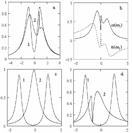
Figure 2: Absorption index at $\omega_{1}$ (reduced by its resonant value in the absence of all strong fields) vs one-photon detunings $\Omega_{1}/\Gamma_{gm}$. Here, $q_{ff}=0.9$, $q_{nn}=0.5$, $\Gamma_{gm}/\Gamma_{gf}=100$, and $\Gamma_{gm}/\Gamma_{gn}=10$. (a,b): $\Omega_{2}=0$, $q_{fn}=1.5$, $g_{mn}=7$, $\gamma_{ff}/\Gamma_{gf}=2$. (a): $\gamma_{nn}=0(1)$, $\gamma_{nn}/\Gamma_{gn}=5$, $\Omega_{L}/\Gamma_{gm}=0.8(2)$. (b): $\gamma_{nn}/\Gamma_{gn}=5$, $\Omega_{L}=0$. (c,d): $\Omega_{2}/\Gamma_{mn}=0.3$, $g_{mn}=70$, $\gamma_{ff}/\Gamma_{gf}=10$, $\Omega_{L}/\Gamma_{gm}=-1.1$, $\gamma_{nn}=0(1)$, $\gamma_{nn}/\Gamma_{gn}=50(2)$. (c): $q_{fn}=15$. (d): $q_{fn}=1.5$.

The factor in the parentheses in the above formula has two singularities with respect to $x_{m}$, which indicates splitting of the resonance into two maxima. The positions of these maxima and their relative amplitudes may vary depending on the parameters of the fields and transitions. Resonance splitting is stipulated by the appearance of coherence at the transition $ng$ and by the consequent appearance of additional quantum transitions in which photons of frequency $\hbar\omega_{1}$ may participate. The phase and relaxation properties of the corresponding term in nonlinear polarization at the frequency $\omega_{1}$ are represented by the dispersion function $X_{n}$. The additional strong fields $E_{3}$ and $E$ perturb the quantum system, which, as pointed out earlier, causes additional modification of the laser-induced quasi-levels and resonances. The changes in the refractive index can he explained similarly.

The spectral characteristics of absorption at the frequency $\omega_{S}$ are governed by the interference between three quantum pathways: directly to the continuum, to level $f$, and also to the superposition of levels $n$ and $m$. The influence of the first two processes was investigated earlier in Refs. GP2 , GP3 , Kn , Vved and is accounted for by the function $\widetilde{A}_{l}$ in the equations (2.19). The strong fields $E_{3}$ and $E_{2}$ lead to additional changes in the spectra. The additional independent structure, described in these expressions by the function $\widetilde{A}_{n}$, is supplemented by the interference structures proportional to the functions $K$ and $U$, which disappear when any of the fields $E_{3}$ or $E$ is turned off or when the spacing between the quasi-levels $\Omega_{L}$ is increased.

Figure 2 shows the dependence of the absorption index at $\omega_{1}$ on the scaled detunings from the bare-state one-photon resonance $\Omega_{1}/\Gamma_{gm}$. The dashed plot at Fig. 2(b) shows the lineshape of the dispersive index at the frequency $\omega_{1}$ for the same parameters. The plot indicates very strong dispersion, induced by the dressing fields coupled to both discrete and continuum states. Figures 2(c) and 2(d) illustrate the sensitivity of the spectra, induced jointly by two dressing fields $E_{3}$ and $E$, on the Fano parameter $q_{fn}$. One can create transparency in certain frequency intervals of the discrete transitions or, on the contrary, eliminate effects of the dressing fields with the aid of destructive interference by varying the intensities and detunings of the driving fields as well as the coupled levels.

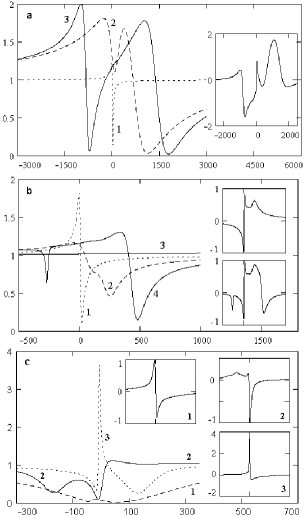
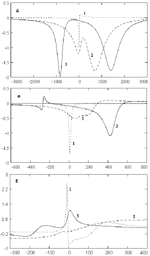
Figure 3: Absorption index at $\omega_{S}$ (reduced by its value in the absence of all strong fields) vs detunings $\Omega/\Gamma_{fg}=(\omega_{S}-\omega-\omega_{fg})/\Gamma_{fg}$ (a-c). The inserts are the interference contributions to the corresponding curves vs detuning (for (b,c) the detuning interval is the same as for the main curves). Here $\Gamma_{gm}/\Gamma_{gf}=100$, $\Gamma_{gm}/\Gamma_{gn}=10$. (a,b): $q_{ff}=0.9$, $q_{nn}=0.9$, $\Omega_{L}/\Gamma_{gf}=-110$, and $\Omega_{2}/\Gamma_{gf}=30$. (a): $q_{gf}=-0.5$, $q_{gn}=-0.95$, $q_{fn}=15$. (b): $q_{gf}=-0.95$, $q_{gn}=-0.5$, $q_{fn}=15$(1,2,3), $q_{fn}=150$(4). (1) $E_{2}=E_{3}=0$, $\gamma_{ff}/\Gamma_{gf}=10$. (2-4) $g_{mn}=70$, $\gamma_{nn}/\Gamma_{gn}=50$. (2) $\gamma_{ff}=0$. (3,4) $\gamma_{ff}/\Gamma_{gf}=10$. (c): $q_{gf}=0.95$, $q_{gn}=0.01$, $q_{ff}=0.01$, $q_{nn}=-5$, $q_{fn}=1.5$, $\Omega_{2}/\Gamma_{gf}=0$, $\gamma_{ff}/\Gamma_{gf}=10$, $\Gamma_{gf}=-1530$. (2,3) $\gamma_{nn}/\Gamma_{gn}=5$. (2) $\Omega_{L}/\Gamma_{gf}=-110$. (3) $\Omega_{L}/\Gamma_{gf}=-405$. (d-f): Scaled dispersive profile of LICS at $\omega_{S}$ vs $\Omega/\Gamma_{fg}$. (All parameters are the same as in plots (a-c), consequently.) In the absence of the driving fields absorption level corresponds to 1, dispersive – to zero.

Figures 3(a) and 3(b) show the dependence of the absorption index at the frequency $\omega_{S}$ (reduced by its value in the absence of the dressing fields) on the scaled detuning $\Omega/\Gamma_{fg}=(\omega_{S}-\omega-\omega_{fg})/\Gamma_{gf}$. The plots indicate the sensitivity of the probe field absorption on the Fano parameters (in the considered cases on $q_{gf}$ and $q_{gn}$) and demonstrate new possibilities for manipulation of LICS with extra dressing fields coupling adjacent transitions. Interference contributions, which disappear in the absence of either the $E$ or $E_{3}$ field, are shown in the inputs to the figure. Figure 3(c) demonstrates the sensitivity of the absorption spectrum on the strength of the driving field $E_{3}$ as well as on the spacing of two quasi-levels, induced in the continuum (on two-photon detuning $\Omega_{L}=\omega-\omega_{3}-\omega_{fn}$). The figures show possible manipulation of LICS in the absorption index for a probe radiation (including formation of transparency windows). This is brought about by the interference of two LICS (quantum pathways via discreet and continuum states), induced by the fields at $\omega_{3}$ and $\omega$ and modified by the strong field at $\omega_{2}$.

The refractive index is proportional to the derivative of the structures over frequency. The plots 3(d,e,f) display the potential of manipulating the magnitude and lineshape of the factor $(n(\omega_{S})-1)/(n_{S\max}-1)$ with the change of intensities and detunings of the dressing fields, as well as strong dependence on the Fano parameters, which may find applications in short-wavelength optics.

The nonlinear interference effects involving quantum transitions may influence differently the linear and nonlinear susceptibilities. Therefore, under certain conditions a reduction in the absorption of the initial and generated radiations can be simultaneously followed by an increase in the nonlinear polarization caused by the resonant effects and by the constructive interference in the strong fields. It is thus possible to increase considerably the power of the generated short-wavelength radiation.

2.4 Resonance sum-frequency generation in strongly-absorbing media enhanced by quantum interference

In weak fields the nonlinear susceptibility increases strongly upon approaching to discrete resonances, but this is accompanied by enhancement of the absorption of the initial radiations. Depending on the detunings from the resonances, on the ratio of the oscillator strengths of the transitions, and on the radiation intensities, either the absorption of the initial radiation $E_{1}$ or of the generated radiation may predominate. A numerical analysis of the influence of these factors on changes in the frequency dependence of the power of the generated short-wavelength radiation during the course of propagation in an optically dense medium can be made if the quantum efficiency of conversion given by expression (2.7) is rewritten in the form:

$$\eta_{\rm q}(z)=\frac{4\overline{\eta}_{{\rm q}0}}{|\overline{b}|}\exp\big{[}-(\overline{\alpha}_{1}+C\overline{\alpha}_{S}){z_{0}}\big{]}\bigg{\{}{\rm sinh}^{2}\bigg{[}\sqrt{{(|\overline{b}|-\overline{b})C/2}}\cdot{z_{0}}\bigg{]}+\sin^{2}\bigg{[}\sqrt{{(\mid\overline{b}\mid+\overline{b})C/2}}\cdot{z_{0}}\bigg{]}\bigg{\}},$$ (2.23)

where $\overline{\eta}_{{\rm q}0}=\tilde{\eta}_{{\rm q}0}/(\alpha_{10}\alpha_{S0}),\>\overline{b}=b/(\alpha_{10}\alpha_{S0})=4\overline{\eta}_{{\rm q}0}-(\overline{\alpha}_{1}-C\overline{\alpha}_{S})^{2}/4C,\>\overline{\alpha}_{1}=\alpha_{1}/\alpha_{10};\>\overline{\alpha}_{S}=\alpha_{S}/\alpha_{S0},\>C=\alpha_{S0}/\alpha_{10},\>andz_{0}=z\alpha_{10}/2$.

The expression for $\overline{\eta}_{{\rm q}0}$, describing the quantum efficiency of conversion over a distance $1/\sqrt{\alpha_{10}\alpha_{S0}}$, considered within the approximation of ignoring absorption of given fields, becomes

$$\overline{\eta}_{{\rm q}0}=\eta_{{\rm q}0}^{0}|\overline{\chi}^{(3)}|^{2}g_{mn}g_{nn},$$ (2.24)

where $\eta_{{\rm q}0}^{0}$ is the quantum efficiency of conversion based on the resonant unperturbed nonlinearity over a distance $1/\sqrt{\alpha_{10}\alpha_{S0}}$ in fields corresponding to $g_{mn}=g_{nn}=1;\>\overline{\chi}^{(3)}=\chi^{(3)}/\chi_{0}$. We shall henceforth use the following approximate expressions:

$$\alpha_{10}=4\pi{\omega_{1}}{|d_{gm}|^{2}/c\hbar\Gamma_{gm}},\>\alpha_{S0}=4\pi^{2}{(\omega_{S}/c)}|d_{g\varepsilon}|^{2}\bigg{|}_{\varepsilon=\hbar\omega_{3}},$$

$$|\chi_{0}|^{2}=(\pi/2\hbar^{2})^{2}(1+q_{gn}^{2})|d_{gm}d_{mn}d_{n\varepsilon}d_{\varepsilon g}|^{2}(\Gamma_{gm}\Gamma_{gn})^{-2}.$$ (2.25)

In this approximation the factor $\eta_{{\rm q}0}^{0}$ is determined completely by the Fano parameter $q_{gn}$:

$$\eta_{{\rm q}0}^{0}=k_{1}^{\prime}k_{S}^{\prime}|2\pi\chi_{0}|^{2}|\big{/}d_{mn}d_{n\varepsilon}|^{2}\pi(16\hbar^{3}\Gamma_{gm}\Gamma_{gn}^{2})^{-1}\alpha_{10}\alpha_{S0}=(1+q_{gn}^{2}).$$ (2.26)

As pointed our earlier, the laser-induced absorption and transparency resonances of the radiation $E_{1}$ can be interpreted as splitting of the level $m$ into quasi-levels by the strong field $E_{2}$ (in combination with the fields $E_{3}$ and $E$). The laser-induced resonances of the generated radiation are determined by two quasi-levels in the continuum and appear near the frequencies $\omega_{ng}+\omega_{3}$ and $\omega_{fg}+\omega$. These quasi-levels are separated by an energy $\hbar\Omega_{L}$. The detuning of the generated radiation frequency from the first resonance amounts to $\Omega_{S}=\Omega_{1}+\Omega_{2}$, and that from the second resonance is $\Omega=\Omega_{S}-\Omega_{L}$. The corresponding quantum channels may interfere differently when the detunings $\Omega_{1},\>\Omega_{2}$ and $\Omega_{L}$ are altered, which is manifested in the spectral characteristics of the absorption and nonlinear-optical generation processes. The relative role of these channels is governed by the intensities of the radiations, by their detunings from the resonances, and by the ratio of the oscillator strengths for the $g-m$ and $g-\varepsilon$ transitions. We shall now illustrate these relationships by considering several numerical models.

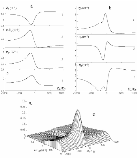
Figure 4: Dependence of the absorption indices $\alpha_{1}/\alpha_{10}$ and $\alpha_{S}/\alpha_{10}$, of the value $\overline{\eta}_{{\rm q}0}$ (that is proportional to the squared modulus of the amplitude of the nonlinear polarization at the entrance to the medium), and of the conversion rate $\overline{b}$ on the detuning $\Omega_{L}$ (a). Dependence of the quantum conversion efficiency $\eta_{\rm q}$ on $\Omega_{L}$ for $z\alpha_{10}=8.5\cdot 10^{3}$ (1), $z\alpha_{10}=1\cdot 10^{4}$ (2), and $z\alpha_{10}=2\cdot 10^{4}$ (3) (b). Dependence of the quantum conversion efficiency $\eta_{\rm q}$ on the optical thickness and on $\Omega_{L}$ (c). Here, $C=10^{-5}$, $g_{ff}=150$, $g_{nn}=200$, $g_{mn}=9000$, $\Omega_{1}/\Gamma_{gf}=5000$, $\Omega_{2}/\Gamma_{gf}=-5100$, $q_{fg}=0.95$, $q_{gn}=-2$, $q_{ff}=0.01$, $q_{nn}=-5$, $q_{fn}=0$, $\Gamma_{gm}/\Gamma_{gf}=100$, $\Gamma_{gm}/\Gamma_{gn}=10$ (a-c).

Figure 4 illustrates the case when the integral oscillator strength for a transition to an energy interval $E$ (of the order of the level widths) in the continuum is considerably less than for the $gm$ transition $(C=10^{-5})$. The frequencies $\omega_{1}$ and $\omega_{2}$ are detuned far from their one-photon transitions, but the frequency sum is close to a perturbed two-photon resonance. It is evident from Fig. 4 that changes in $\Omega_{L}$ (because of variation of the frequencies $\omega$ or $\omega_{3}$) reduce, for the selected Fano parameters and radiations, the absorption coefficient $\alpha_{1}$ by approximately threefold, increase $\alpha_{S}$ approximately by a factor of 3.8 in one detuning interval, and reduce considerably this coefficient in the other interval, whereas the square of the modulus of the nonlinear polarization (proportional to $\overline{\eta}_{{\rm q}0}$) increases by a factor of 1.9 (these changes are relative to the values of the corresponding parameters in the far wings where the effects of the strong field $E$ do not appear) [Fig. 4 (a)]. The absorption coefficient for a transition to the continuum remains on the whole much less than $\alpha_{1}$ ($\alpha_{S}/\alpha_{1}=C\overline{\alpha}_{S}/\overline{\alpha}_{1}\approx 10^{-2}$). In a certain range of $\Omega_{L}$, the sign of $\overline{b}$ becomes positive, and the nonlinear-optical conversion rate begins to exceed the rate of absorption of the radiation. It is in this interval that there is a sharp maximum of the quantum efficiency of conversion (the dependence of this conversion efficiency on the optical thickness and on $\Omega_{L}$ is demonstrated in Fig. 4 (c), where the maximum $\eta_{{\rm q}\max}=0.29$ is reached for $z\alpha_{10}=4000$). The absorption of the radiation $E_{1}$ alters considerably the dependence of the power of the generated radiation on $\Omega_{L}$ along the medium [Fig. 4 (b)].

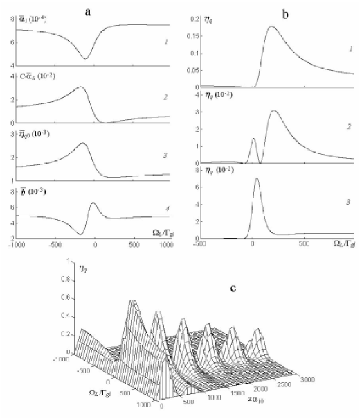
Figure 5: Absorption indices $\alpha_{1}/\alpha_{10}$ and $\alpha_{S}/\alpha_{10}$, the value $\overline{\eta}_{{\rm q}0}$ and conversion rate $\overline{b}$ plotted as a function of $\Omega_{L}$ (a). Dependence of the quantum conversion efficiency $\eta_{\rm q}$ on $\Omega_{L}$ along the medium computed for $z\alpha_{10}=4.5\cdot 10^{2}$ (1), $z\alpha_{10}=5\cdot 10^{2}$ (2), and $z\alpha_{10}=5.5\cdot 10^{2}$ (3) (b). Dependence of $\eta_{\rm q}$ on the optical thickness and on $\Omega_{L}$ (c). Here, $C=3\cdot 10^{-2}$, $g_{nn}=500$, $g_{mn}=8000$ (a-c). The other parameters are the same as in Fig. 4.

Figure 5 is computed for the case where the detuning from a one-photon resonance is still large, but the oscillator strengths for a discrete transition and a transition to the continuum differ less $(C=3\cdot 10^{-2})$. Then, under the action of the field $E$, variation of $\Omega_{L}$ can reduce the absorption coefficient $\alpha_{1}$ by a factor of just 1.5, whereas the absorption coefficient $\alpha_{S}$ increases approximately threefold in one interval, but falls considerably in the other interval; practically throughout the whole range of the detuning $\Omega_{L}$, the dominant effect is the absorption transition into the continuum ($\alpha_{S}/\alpha_{1}\approx 70$), and $\overline{\eta}_{{\rm q}0}$ increases by a factor of 1.9 [Fig. 5(a)]. The quantity $\overline{b}$ is always positive and has a characteristic maximum in a certain interval of $\Omega_{L}$. For a given detuning, the rate of conversion begins to exceed the rate of absorption so much that an oscillatory regime appears along the medium. Propagation in an optically-dense medium makes the spectrum of the output power significantly dependent on the optical length of the medium, i.e., on $z$ or on the concentration $N$ of atoms. The absolute amplitude and the position of the maximum change, and new resonances appear [Fig. 5(b)]. At the first maximum (corresponding to $z\alpha_{10}\approx 125$) the quantum efficiency of conversion can reach 0.9 [Fig. 5(c)], which is three times greater than in the preceding case.

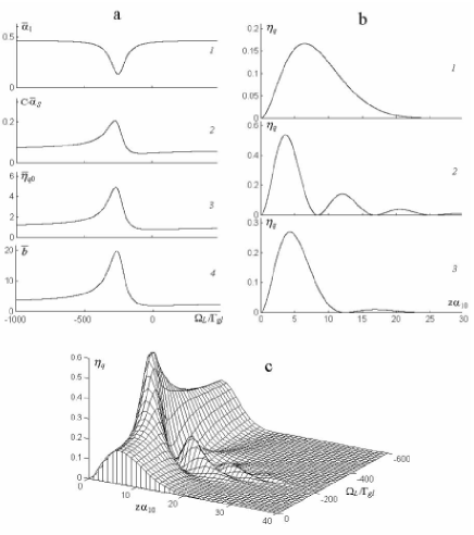
Figure 6: Dependence of the absorption indices $\alpha_{1}/\alpha_{10}$ and $\alpha_{S}/\alpha_{10}$, of the value $\overline{\eta}_{{\rm q}0}$, and of the conversion rate $\overline{b}$ on $\Omega_{L}$ (a). Dependence of the quantum conversion efficiency $\eta_{\rm q}$ on the optical thickness for $\Omega_{L}/\Gamma_{gf}=0$ (1), $\Omega_{L}/\Gamma_{gf}=-250$ (2), $\Omega_{L}/\Gamma_{gf}=-400$ (3) (b). Dependence of the quantum conversion efficiency $\eta_{\rm q}$ on the optical thickness and on $\Omega_{L}$ (c). Here, $g_{ff}=100$, $g_{nn}=5$, $g_{mn}=7$, $\Omega_{1}/\Gamma_{gf}=0$, $\Omega_{2}/\Gamma_{gf}=-250$ (a-c). The other parameters are the same as in Fig. 5.

In view of the nonresonant nature of the interaction, the attainment of such high values of the quantum efficiency of conversion requires high intensities of the $E_{2}$ and $E_{3}$, radiations, and also long lengths (or high densities of atoms) of the medium. The use of resonant processes makes it possible to reduce the required intensities and to reach considerable values of the quantum efficiency by optimization of the bleaching and interference effects. Figure 6 illustrates the case where the ratio of oscillator strengths is the same as in Fig. 5, but there is no detuning from a one-photon resonance. At intensities of the $E_{2}$ radiation three orders of magnitude less than in the preceding case, it is possible to reduce the absorption coefficient of the $E_{1}$ radiation approximately by a factor of 10 compared with the value of this coefficient in the absence of strong fields (the maximum effect of the field $E$ is a reduction in this coefficient by a factor of 1.5) [Fig. 6(a)]. In the region of reduction in $\alpha_{1}$, the value of $\alpha_{S}$ increases approximately threefold and $\overline{\eta}_{{\rm q}0}$ by a factor of 4.7. The absorption coefficients $\alpha_{1}$ and $\alpha_{S}$ are then comparable, and the nonlinear-optical conversion rate exceeds considerably, in a wide range of $\Omega_{L}$, the rates of absorption of the radiations, reaching a sharp maximum at $\Omega_{L}/\Gamma_{gf}=-250$. This gives rise to an oscillatory regime of generation along the medium in this detuning range [Figs. 6(b,c)], i.e., it leads to the feasibility of total (apart from that lost by absorption) conversion of the radiations $E_{1}$ and $E_{S}$ (and vice versa) for certain products of the length of the medium and the concentration of atoms. For the selected parameters, the conversion efficiency at the first maximum (where $z\alpha_{10}\approx 5$) reaches 0.54. This is less than in the preceding case because of the much greater absolute values of the absorption coefficient, but this efficiency is reached at much lower intensities and for much smaller lengths of the nonlinear medium and much lower concentration of atoms in this medium.

2.5 Absorption and dispersive spectra at Doppler-broadened transitions

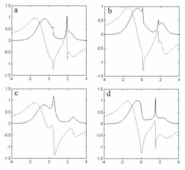
Figure 7: Absorption (solid) and refractive (dash) indices at $\omega_{1}$ (reduced by its value in the absence of all strong fields) in a Doppler-broadened medium vs detunings $\Omega_{1}/\Delta\omega_{1D}$. Here, the Doppler HWHM $\Delta\omega_{1D}=16.65\Gamma_{gm}$, the wavevector orientations are ${\bf k}\uparrow\uparrow{\bf k}_{1}$, ${\bf k}_{2}\uparrow\uparrow{\bf k}_{3}\uparrow\downarrow{\bf k}_{1}$, and $k_{2}/k_{1}=0.9$, $k_{3}/k_{1}=0.5$, $k/k_{1}=0.6$ (${\bf k}_{i}$ is wave-vector corresponding to the frequency $\omega_{i}$), $\Gamma_{gm}/\Gamma_{gf}=100$, $\Gamma_{gm}/\Gamma_{gn}=10$; $|G_{mn}|^{2}/(\Delta\omega_{1D})^{2}=1$, $q_{nn}=0.5$, $q_{ff}=0.9$, $\Omega_{2}/\Delta\omega_{1D}=9$. (a,b): $\gamma_{nn}/\Delta\omega_{1D}=0.2$, $\gamma_{ff}/\Delta\omega_{1D}=0.1$, $q_{fn}=0.5$. (a): $\Omega_{L}=0$. (b-d): $\Omega_{L}/\Delta\omega_{1D}=-0.8$. (c): $\gamma_{nn}/\Delta\omega_{1D}=0.8$, $\gamma_{ff}/\Delta\omega_{1D}=0.3$, $q_{fn}=-1.5$. (d): $\gamma_{nn}/\Delta\omega_{1D}=0.2$, $\gamma_{ff}/\Delta\omega_{1D}=0.8$, $q_{fn}=1.5$.

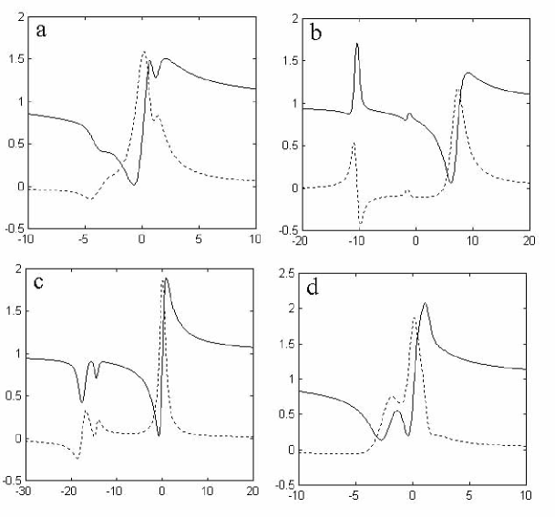
Figure 8: Absorption (solid) and refractive (dash) indices at $\omega_{S}$ (reduced by its value in the absence of all strong fields) at Doppler-broadened transitions vs detunings $\Omega/\Delta\omega_{4D}=(\omega_{S}-\omega-\omega_{fg})/\Delta\omega_{SD}$. Here, the Doppler HWHM $\Delta\omega_{SD}=5\cdot 10^{3}\Gamma_{gf}$; the wavevector orientations are ${\bf k}\uparrow\uparrow{\bf k}_{3}\uparrow\uparrow{\bf k}_{2}\uparrow\uparrow{\bf k}_{4}$, and $k/k_{4}=0.8$, $k_{3}/k_{4}=0.3$, $k_{2}/k_{4}=0.37$, $\Gamma_{gm}/\Gamma_{gf}=100$, $\Gamma_{gm}/\Gamma_{gn}=10$; $|G_{mn}|^{2}/(\Delta\omega_{SD})^{2}=1$, $\gamma_{nn}/\Delta\omega_{SD}=0.4$, $\gamma_{ff}/\Delta\omega_{SD}=0.8$, $q_{gf}=0.95$, $q_{gn}=0.01$, $q_{ff}=0.01$, $q_{nn}=-5$. (a): $q_{fn}=1.5$, $\Omega_{L}/\Delta\omega_{SD}=1.5$, $\Omega_{2}/\Delta\omega_{SD}=2.2$. (b-d): $\Omega_{2}=0$. (b): $q_{fn}=15$, $\Omega_{L}/\Delta\omega_{SD}=1.5$. (c): $q_{fn}=-1.5$, $\Omega_{L}/\Delta\omega_{SD}=15$. (d): $q_{fn}=-1.5$, $\Omega_{L}/\Delta\omega_{SD}=-0.5$.

A Lorentzian line profile with near natural linewidth can be observed only by making use special techniques, like atomic jets. Analysis shows that the contributions of atoms at different velocities in a Doppler-broadened medium may completely change the features described above. Figures 7 and 8 demonstrate that proper adjustment of the orientation of the wavevectors, along with the intensities and detunings of the coupled waves, provides additional means to manipulate the lineshape. Moreover, enhanced subDoppler structures can be formed by the compensation for Doppler shifts by power shifts. For details of the physics, see Sh , Ba and references therein. The plots dshow that the interference of contributions from the atoms at different velocities brings an important distinction in appearance of quantum interference processes at coupled discrete and continuous states. The figures show that the appearance of quantum interference at Doppler-broadened transitions also may be both constructive and distractive, depending on the detunings of $\omega-\omega_{3}$ from $\omega_{nf}$, on the Fano parameters, on the detunings from the two-photon resonance $gn$, on the ratios of the wavenumbers, and on orientations of the wavevectors.

3 Four-wave mixing, dissociation and population transfer controlled by LICS in folded energy-level schemes

Here, we will consider the folded scheme, which is characteristic for molecules with low-lying predissociation states. Such a coupling configuration allows coherent laser control of dissociation through the ’dark’ states that are not connected with the ground one by the allowed transition. On the other hand, the scheme under consideration enables one to transfer the population between two upper bound states which are not connected directly too. Thus, we will explore the possibilities of manipulating dissociation and populations of excited states through implementation of the interference of quantum pathways via a variety of low-lying continuum states.

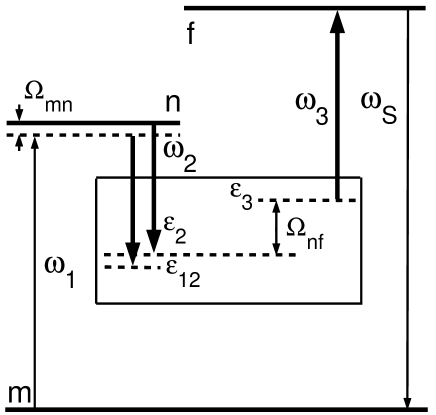
Figure 9: LICS-based coherent control in the folded schemes.

The proposed coupling scheme is illustrated in the energy level diagram depicted in Fig. 9. The radiation at frequency $\omega_{1}$ couples the bound-bound transition $m-n$, and radiations at the frequencies $\omega_{2}$ and $\omega_{3}$ couple the bound states $n$ and $f$ with the states of dissociation continuum $\varepsilon$, as shown in the picture. Density matrix equations, which are employed for investigating population transfer, account for both relaxation and incoherent excitation of the discrete states:

$$\dot{\rho}_{n\varepsilon}=i\left(\rho_{nn}V_{n\varepsilon}+\rho_{nf}V_{f\varepsilon}\right),$$

$$\dot{\rho}_{f\varepsilon}=i\left(\rho_{ff}V_{f\varepsilon}+\rho_{fn}V_{n\varepsilon}\right),$$

$$\dot{\rho}_{m\varepsilon}=i\left(\rho_{mn}V_{n\varepsilon}+\rho_{mf}V_{f\varepsilon}\right),$$

$$\dot{\rho}_{mn}+\Gamma_{mn}\rho_{mn}=i\left(\rho_{mm}V_{mn}+\int d\varepsilon\rho_{m\varepsilon}V_{\varepsilon n}-V_{mn}\rho_{nn}\right),$$

$$\dot{\rho}_{mf}+\Gamma_{mf}\rho_{mf}=i\left(\int d\varepsilon\rho_{m\varepsilon}V_{\varepsilon f}-V_{mn}\rho_{nf}\right),$$ (3.27)

$$\dot{\rho}_{nf}+\Gamma_{nf}\rho_{nf}=i\left(\int d\varepsilon\rho_{n\varepsilon}V_{\varepsilon f}-\int d\varepsilon V_{n\varepsilon}\rho_{\varepsilon f}-V_{nm}\rho_{mf}\right),$$

$$\dot{\rho}_{\varepsilon\varepsilon}=-2\hbox{Re\,}\left(i\int d\varepsilon V_{\varepsilon n}\rho_{n\varepsilon}+i\int d\varepsilon V_{\varepsilon f}\rho_{f\varepsilon}\right),$$

$$\dot{\rho}_{nn}+\Gamma_{n}\rho_{nn}=-2\hbox{Re\,}\left(i\int d\varepsilon V_{n\varepsilon}\rho_{\varepsilon n}+iV_{nm}\rho_{mn}\right)+Q_{n},$$

$$\dot{\rho}_{ff}+\Gamma_{f}\rho_{ff}=-2\hbox{Re\,}\left(i\int d\varepsilon V_{f\varepsilon}\rho_{\varepsilon f}\right)+Q_{f},$$ (3.28)

$$\dot{\rho}_{mm}+\Gamma_{m}\rho_{mm}=-2\hbox{Re\,}\left(iV_{mn}\rho_{nm}\right)+Q_{m}+w_{nm}\rho_{nn}.$$

Here, $Q_{i}$ is the rate of incoherent excitation to level $i$, $\Gamma_{i}\rho_{ii}$ is the rate of relaxation, $w_{nm}$ is the probability of excitation of level $m$ due to the relaxation transitions from level $n$, and $V_{jk}$ and $V_{j\varepsilon}$ are the corresponding matrix elements of the quasi-resonant electrodipole interaction of the driving field and molecules scaled to Planck’s constant $\hbar$. The system of equations (3.28) corresponds to the case of an open energy level configuration. This implies that all the levels coupled with the driving fields, including level $m$, can be incoherently excited from the reservoir of much greater populated lower levels, so that the parameters $Q_{j}$ are constant.

For the closed schemes, i.e., the schemes where level $m$ is a ground one, and therefore incoherent excitation of the upper levels depends on population transfer stimulated by the applied fields, the equations for the populations take the form

$$\dot{\rho}_{ff}+\Gamma_{f}\rho_{ff}=-2\hbox{Re\,}\left(i\int d\varepsilon V_{f\varepsilon}\rho_{\varepsilon f}\right)+w_{f}\rho_{mm},$$

$$\dot{\rho}_{nn}+\Gamma_{n}\rho_{nn}=-2\hbox{Re\,}\left(i\int d\varepsilon V_{n\varepsilon}\rho_{\varepsilon n}+iV_{nm}\rho_{mn}\right)+w_{n}\rho_{mm},$$ (3.29)

$$\rho_{mm}=1-\rho_{nn}-\rho_{ff}-\int\dot{W}dt.$$

Here, $w_{i}$ describes the probability of excitation to level $i$ from the ground state, and $\dot{W}$ is rate of dissociation.

In the equations (3.27), the terms like $\rho_{\varepsilon k}V_{kj}$ ($j,k=n,m$) are discarded. This is valid because coherence at discrete-discrete two-photon transitions is usually much stronger than that at bound-free two-photon transitions. The driving fields couple the interval of continuum states in the vicinity of the resonant energy $\varepsilon_{0}$ that is roughly equal to the width of the coupled power-broadened discrete levels. However, the oscillation strength at a bound-free transition is distributed over a much wider energy interval. Therefore, the fraction of oscillator strength attributed to the coupled energy interval is usually relatively small. The requirement derived with the aid of the Laplace transformation indicates that the indicated terms in the above equations can be neglected until

$${\partial f}/{\partial\varepsilon_{\varepsilon=\varepsilon_{0}}}>>\hbar|V_{jk}|{\partial^{2}f}/{\partial\varepsilon^{2}_{\varepsilon=\varepsilon_{0}}},$$ (3.30)

where $f(\varepsilon)$ is the energy density of the transition oscillator strength. Such a requirement is fulfilled practically for all realistic atomic and molecular continua in the energy range that is well above the ionization or dissociation threshold.

3.1 Quasistationary solution of density matrix equations

In this section we shall assume that all radiations are continuous waves or rectangular pulses with duration $\tau$ that is much greater than all relaxation times in the quantum system under investigation. We will consider also the case of small loss of molecules due to dissociation for the period of measurement or the pulse duration, so that the quasi-stationary regime is established. The corresponding requirement is

$$\int\limits_{0}^{\tau}\dot{W}dt=W(\tau)<<1,$$ (3.31)

where the dissociation yield $\dot{W}dt$ is described by the equation

$$\dot{W}=\dot{\rho}_{\varepsilon}=-2\hbox{Re\,}\left(i\int d\varepsilon V_{\varepsilon n}\rho_{n\varepsilon}+i\int d\varepsilon V_{\varepsilon f}\rho_{f\varepsilon}\right).$$ (3.32)

Quasi-stationary solutions of the density matrix can be found in the form

$$\rho_{ii}=r_{i}\quad(i=m,n,f),\quad\rho_{ij}=r_{ij}\exp(i\Omega_{ij}t),\quad\rho_{j\varepsilon}=r_{j\varepsilon}\exp(i\Omega_{j\varepsilon}t),$$

$$V_{ij}=G_{ij}\exp(i\Omega_{ij}t),\quad V_{j\varepsilon}=G_{j\varepsilon}\exp(i\Omega_{j\varepsilon}t).$$ (3.33)

Here, $G_{ij}=E_{k}d_{ij}/2\hbar$, $G_{j\varepsilon}=E_{k}d_{j\varepsilon}/2\hbar$, $\Omega_{mn}=\omega_{1}-\omega_{mn}$, $\Omega_{nf}=\omega_{3}-\omega_{2}-\omega_{nf}$, $\Omega_{mf}=\omega_{1}-\omega_{2}+\omega_{3}-\omega_{mf}$, $\Omega_{n\varepsilon}=\omega_{2}-\omega_{n\varepsilon}$, $\Omega_{f\varepsilon}=\omega_{3}-\omega_{f\varepsilon}$, and $\Omega_{m\varepsilon}=\omega_{1}-\omega_{2}-\omega_{m\varepsilon}$. The amplitudes of the resonant fields $E_{k}$ (see Fig. 9), and consequently all amplitudes $r_{i}$, $r_{ij}$, and $r_{j\varepsilon}$, are assumed to be independent of time. Then, by introducing the expressions (3.33) to the equations (3.27), we can reduce them to a system of algebraic ones:

$$ir_{n\varepsilon}p_{n\varepsilon}=-r_{n}G_{n\varepsilon}-r_{nf}G_{f\varepsilon},\quad p_{n\varepsilon}=i(\omega_{2}-\omega_{n\varepsilon});$$

$$ir_{f\varepsilon}p_{f\varepsilon}=-r_{f}G_{f\varepsilon}-r_{fn}G_{n\varepsilon},\quad p_{f\varepsilon}=i(\omega_{3}-\omega_{f\varepsilon});$$

$$ir_{m\varepsilon}p_{m\varepsilon}=-r_{mn}G_{n\varepsilon}-r_{mf}G_{f\varepsilon},\quad p_{m\varepsilon}=i(\omega_{1}-\omega_{2}-\omega_{m\varepsilon});$$

$$ir_{mn}p_{mn}=-\int d\varepsilon r_{m\varepsilon}G_{\varepsilon n}-r_{m}G_{mn}+G_{mn}r_{n},\quad p_{mn}=\Gamma_{mn}+i(\omega_{1}-\omega_{mn});$$ (3.34)

$$ir_{mf}p_{mf}=-\int d\varepsilon r_{m\varepsilon}G_{\varepsilon f}+G_{mn}r_{nf},\quad p_{mf}=\Gamma_{mf}+i(\omega_{1}-\omega_{2}+\omega_{3}-\omega_{mf});$$

$$ir_{nf}p_{nf}=-\int d\varepsilon r_{n\varepsilon}G_{\varepsilon f}+\int d\varepsilon G_{n\varepsilon}r_{\varepsilon f}+G_{nm}r_{mf},\quad p_{nf}=\Gamma_{fn}\pm i(\omega_{3}-\omega_{2}-\omega_{nf}).$$

Further by introducing the solutions of the first, second and third equations to the integrals and with the aid of the $\zeta$-function (2.14), we obtain

$$r_{mn}\left[\delta_{nn}^{m}-\Omega_{mn}+i(\Gamma_{mn}+\gamma_{nn}^{m})\right]=\left(r_{n}-r_{m}\right)G_{mn}-r_{mf}\left(\delta_{fn}^{m}+i\gamma_{fn}^{m}\right),$$

$$r_{mf}\left[\delta_{ff}^{m}-\Omega_{mf}+i(\Gamma_{mf}+\gamma_{ff}^{m})\right]=G_{mn}r_{nf}-r_{mn}\left(\delta_{nf}^{m}+i\gamma_{nf}^{m}\right),$$ (3.35)

$$r_{nf}\left[\delta_{ff}^{n}-\delta_{nn}^{f}-\Omega_{nf}+i(\Gamma_{nf}+\gamma_{ff}^{n}+\gamma_{nn}^{f})\right]=G_{nm}r_{mf}+r_{f}\left(\delta_{nf}^{f}-i\gamma_{nf}^{f}\right)-r_{n}\left(\delta_{nf}^{n}+i\gamma_{nf}^{n}\right),$$

where

$$\gamma_{nn}^{m}=\pi\hbar G_{n\varepsilon_{12}}G_{\varepsilon_{12}n}+\hbox{Re\,}\left(G_{nk}G_{kn}/p_{mk}\right),$$

$$\delta_{nn}^{m}=\hbar{\cal P}\int d\varepsilon\cdot G_{n\varepsilon}G_{\varepsilon n}/(\varepsilon_{12}-\varepsilon)+\hbox{Im\,}\left(G_{nk}G_{kn}/p_{mk}\right);$$

$$\gamma_{ff}^{m}=\pi\hbar G_{f\varepsilon_{12}}G_{\varepsilon_{12}f}+\hbox{Re\,}\left(G_{fk}G_{kf}/p_{mk}\right),$$

$$\delta_{ff}^{m}=\hbar{\cal P}\int d\varepsilon\cdot G_{f\varepsilon}G_{\varepsilon f}/(\varepsilon_{12}-\varepsilon)+\hbox{Im\,}\left(G_{fk}G_{kf}/p_{mk}\right);$$

$$\gamma_{nf}^{m}=\pi\hbar G_{n\varepsilon_{12}}G_{\varepsilon_{12}f}+\hbox{Re\,}\left(G_{nk}G_{kf}/p_{mk}\right),$$ (3.36)

$$\delta_{nf}^{m}=\hbar{\cal P}\int d\varepsilon\cdot G_{n\varepsilon}G_{\varepsilon f}/(\varepsilon_{12}-\varepsilon)+\hbox{Im\,}\left(G_{nk}G_{kf}/p_{mk}\right);$$

$$\gamma_{fn}^{m}=\pi\hbar G_{f\varepsilon_{12}}G_{\varepsilon_{12}n}+\hbox{Re\,}\left(G_{fk}G_{kn}/p_{mk}\right),$$

$$\delta_{fn}^{m}=\hbar{\cal P}\int d\varepsilon\cdot G_{f\varepsilon}G_{\varepsilon n}/(\varepsilon_{12}-\varepsilon)+\hbox{Im\,}\left(G_{fk}G_{kn}/p_{mk}\right);$$

$$\gamma_{nn}^{n}=\pi\hbar G_{n\varepsilon_{2}}G_{\varepsilon_{2}n}+\hbox{Re\,}\left(G_{nk}G_{kn}/p_{kn}\right),$$

$$\delta_{nn}^{n}=\hbar{\cal P}\int d\varepsilon\cdot G_{n\varepsilon}G_{\varepsilon n}/(\varepsilon_{2}-\varepsilon)+\hbox{Im\,}\left(G_{nk}G_{kn}/p_{kn}\right);$$

$$\gamma_{ff}^{n}=\pi\hbar G_{f\varepsilon_{2}}G_{\varepsilon_{2}f}+\hbox{Re\,}\left(G_{fk}G_{kf}/p_{kn}\right),$$

$$\delta_{ff}^{n}=\hbar{\cal P}\int d\varepsilon\cdot G_{f\varepsilon}G_{\varepsilon f}/(\varepsilon_{2}-\varepsilon)+\hbox{Im\,}\left(G_{fk}G_{kf}/p_{kn}\right);$$

$$\gamma_{nf}^{n}=\pi\hbar G_{n\varepsilon_{2}}G_{\varepsilon_{2}f}+\hbox{Re\,}\left(G_{nk}G_{kf}/p_{kn}\right),$$ (3.37)

$$\delta_{nf}^{n}=\hbar{\cal P}\int d\varepsilon\cdot G_{n\varepsilon}G_{\varepsilon f}/(\varepsilon_{2}-\varepsilon)+\hbox{Im\,}\left(G_{nk}G_{kf}/p_{kn}\right);$$

$$\gamma_{fn}^{n}=\pi\hbar G_{f\varepsilon_{2}}G_{\varepsilon_{2}n}+\hbox{Re\,}\left(G_{fk}G_{kn}/p_{kn}\right),$$

$$\delta_{fn}^{n}=\hbar{\cal P}\int d\varepsilon\cdot G_{f\varepsilon}G_{\varepsilon n}/(\varepsilon_{2}-\varepsilon)+\hbox{Im\,}\left(G_{fk}G_{kn}/p_{kn}\right);$$

$$\gamma_{nn}^{f}=\pi\hbar G_{n\varepsilon_{3}}G_{\varepsilon_{3}n}+\hbox{Re\,}\left(G_{nk}G_{kn}/p_{kf}\right),$$

$$\delta_{nn}^{f}=\hbar{\cal P}\int d\varepsilon\cdot G_{n\varepsilon}G_{\varepsilon n}/(\varepsilon_{3}-\varepsilon)+\hbox{Im\,}\left(G_{nk}G_{kn}/p_{kf}\right);$$

$$\gamma_{ff}^{f}=\pi\hbar G_{f\varepsilon_{3}}G_{\varepsilon_{3}f}+\hbox{Re\,}\left(G_{fk}G_{kf}/p_{kf}\right),$$

$$\delta_{ff}^{f}=\hbar{\cal P}\int d\varepsilon\cdot G_{f\varepsilon}G_{\varepsilon f}/(\varepsilon_{3}-\varepsilon)+\hbox{Im\,}\left(G_{fk}G_{kf}/p_{kf}\right);$$

$$\gamma_{nf}^{f}=\pi\hbar G_{n\varepsilon_{3}}G_{\varepsilon_{3}f}+\hbox{Re\,}\left(G_{nk}G_{kf}/p_{kf}\right),$$ (3.38)

$$\delta_{nf}^{f}=\hbar{\cal P}\int d\varepsilon\cdot G_{n\varepsilon}G_{\varepsilon f}/(\varepsilon_{3}-\varepsilon)+\hbox{Im\,}\left(G_{nk}G_{kf}/p_{kf}\right);$$

$$\gamma_{fn}^{f}=\pi\hbar G_{f\varepsilon_{3}}G_{\varepsilon_{3}n}+\hbox{Re\,}\left(G_{fk}G_{kn}/p_{kf}\right),$$

$$\delta_{fn}^{f}=\hbar{\cal P}\int d\varepsilon\cdot G_{f\varepsilon}G_{\varepsilon n}/(\varepsilon_{3}-\varepsilon)+\hbox{Im\,}\left(G_{fk}G_{kn}/p_{kf}\right).$$

and

$$\varepsilon_{12} =\hbar(\omega_{1}-\omega_{2}),\quad\varepsilon_{2}=E_{n}-\hbar\omega_{2},\quad\varepsilon_{3}=E_{f}-\hbar\omega_{3},$$ (3.39)

$$p_{mk} =\Gamma_{mk}+i(\omega_{1}-\omega_{2}-\omega_{mk}),\quad p_{kn}=\Gamma_{kn}+i(\omega_{kn}-\omega_{2}),\quad p_{kf}=\Gamma_{kf}+i(\omega_{kf}-\omega_{3}).$$

Besides the continuum states, a contribution of other non-resonant levels $k$ is taken into account too and a sum over repeating $k$ index is assumed. The contribution from these levels may occur commensurable to that of the continuum states. As seen from the equations (3.35), the values $\gamma_{ij}$ and $\delta_{ij}$ describe light-induced broadening and shifts of discrete resonances stipulated by the induced transitions between them through the continuum. The parameters $q_{ij}=\delta_{ij}/\gamma_{ij}$ are analogous to the Fano parameters for autoionizing states. Within the validity of (3.30), their dependence on the field intensities can be neglected. These parameters determine the most important features of the processes under investigation since they characterize the relative integrated contribution of all off-resonant quantum states compared to the resonant ones.

With the aid of (3.34), the equation for the dissociation rate (3.32) takes the form

$$\dot{W}=\dot{r}_{\varepsilon}=2\left[\gamma_{nn}^{n}r_{n}+\gamma_{ff}^{f}r_{f}+2\hbox{Re\,}(\gamma_{fn}r_{nf})\right].$$ (3.40)

The first two terms on RHS describe induced transitions to the continuum from the corresponding discrete levels, whose populations are determined by a variety of processes. Most important is the last term describing quantum interference, which occurs if two LICS overlap. Let us consider specific features of the processes in both open and closed energy level configurations.

3.1.1 Open configuration

In this case in the same way as above, one obtains

$$r_{m}\Gamma_{m}=w_{nm}r_{n}+Q_{m}-2\hbox{Re\,}(iG_{mn}r_{nm}),$$

$$r_{f}(\Gamma_{f}+2\gamma_{ff}^{f})=Q_{f}-2\hbox{Re\,}\left(r_{nf}[\gamma_{fn}^{f}+i\delta_{fn}^{f}]\right),$$ (3.41)

$$r_{n}(\Gamma_{n}+2\gamma_{nn}^{n})=Q_{n}-2\hbox{Re\,}\left(iG_{nm}r_{mn}+r_{nf}[(\gamma_{fn}^{n}-i\delta_{fn}^{n}]\right).$$

Then the solution of (3.35) and (3.41) can be presented in the form

$$r_{nf}={\left\{(r_{n}-r_{m})|G_{mn}|^{2}\gamma_{nf}^{m}(1-iq_{nf}^{m})-[r_{f}\gamma_{nf}^{f}(1+iq_{nf}^{f})+r_{n}\gamma_{nf}^{n}(1-iq_{nf}^{n})]Y\right\}}Z^{-1},$$

$$r_{m}=(L_{1}C_{1}+L_{2}S_{1})/(C_{1}C_{2}-S_{1}S_{2}),\,r_{n}=(L_{2}+S_{2}r_{m})/C_{1},$$

$$r_{f}=[Q_{f}+2r_{n}B_{4}^{fn}+2(r_{m}-r_{n})M_{4}^{fm}]Y_{f}^{-1}.$$ (3.42)

The notations introduced here are as follows:

$$C_{1}=Y_{nm}Y_{f}-L_{1}L_{2},\,C_{2}=[\Gamma_{m}+2(G-M_{1}^{mm})]Y_{f}-4M_{4}^{fm}M_{3}^{mf},$$

$$S_{1}=[w_{nm}+2(G+M_{1}^{mn}-D)]Y_{f}+2L_{2}M_{3}^{mf},\,S_{2}=PY_{f}+2M_{4}^{fm}L_{1},$$

$$F_{1}=Q_{m}Y_{f}+2Q_{f}M_{3}^{mf},\quad F_{2}=Q_{n}Y_{f}-Q_{f}L_{1},\,P=2(G-M_{1}^{nm}+D),$$

$$L_{1}=2(B_{3}^{nf}-2M_{3}^{mf}),\,L_{2}=2(B_{4}^{fn}-M_{4}^{fm}),\,Y_{f}=\widetilde{\Gamma}_{f}-2B_{2}^{ff},$$

$$Y_{nm}=\widetilde{\Gamma}_{n}+2(G-B_{1}^{nn}+M_{1}^{mn}-D),\,G=|G_{mn}|^{2}\hbox{Re\,}(y_{mf}/Y),$$

$$B_{i}^{jl}=\gamma_{nn}^{j}\gamma_{nn}^{l}\hbox{Re\,}(b_{i}^{jl}Y/Z),\,M_{i}^{jl}=|G_{mn}|^{2}\gamma_{nn}^{j}\gamma_{ff}^{l}\hbox{Re\,}(b_{i}^{jl}/Z),$$

$$D=|G_{mn}|^{4}\gamma_{nn}^{m}\gamma_{ff}^{m}\hbox{Re\,}[k_{1}^{mm}/(YZ)],\,j,l=m,n,f;$$

$$Y=y_{mn}y_{mf}-\gamma_{nn}^{m}\gamma_{ff}^{m}b_{1}^{mm},\,Z=y_{mf}y_{nf}y_{mn}-\gamma_{nn}^{m}\gamma_{ff}^{m}b_{1}^{mm}y_{nf}+|G_{mn}|^{2}y_{mn},$$

$$y_{mn}=\widetilde{\Gamma}_{mn}+i(\Omega_{mn}-\delta_{nn}^{m}),\,y_{mf}=\widetilde{\Gamma}_{mf}+i(\Omega_{mf}-\delta_{ff}^{m}),$$

$$y_{nf}=\widetilde{\Gamma}_{nf}+i(\Omega_{nf}+\delta_{nn}^{f}-\delta_{ff}^{n}),\,b_{1}^{jl}=k_{o}(1-iq_{fn}^{j})(1-iq_{nf}^{l}),$$

$$b_{2}^{jl}=k_{o}(1+iq_{fn}^{j})(1+iq_{nf}^{l}),\,b_{3}^{jl}=k_{o}(1-iq_{fn}^{j})(1+iq_{nf}^{l}),$$

$$b_{4}^{jl}=k_{o}(1+iq_{fn}^{j})(1-iq_{nf}^{l}),\,k_{o}=(\gamma_{nf}^{j}\gamma_{fn}^{l})/(\gamma_{nn}^{j}\gamma_{ff}^{l}),\,\widetilde{\Gamma}_{nf}=\Gamma_{nf}+\gamma_{nn}^{f}+\gamma_{ff}^{n},$$

$$\widetilde{\Gamma}_{mn}=\Gamma_{mn}+\gamma_{nn}^{m},\,\widetilde{\Gamma}_{mf}=\Gamma_{mf}+\gamma_{ff}^{m},\,\widetilde{\Gamma}_{n}=\Gamma_{n}+2\gamma_{nn}^{n}+w_{nm},\,\widetilde{\Gamma}_{f}=\Gamma_{f}+2\gamma_{ff}^{f}.$$ (3.43)

First, consider the effect of the interference of two LICS in the case where the laser field at discrete transition is turned off ($G_{mn}=0$). Then the solution (3.42) takes the more simple form of

$$r_{nf}=-[r_{f}\gamma_{nf}^{f}(1+iq_{nf}^{f})+r_{n}\gamma_{nf}^{n}(1-iq_{nf}^{n})]y_{nf}^{-1},\,r_{m}=Q_{m}/\Gamma_{m}+w_{nm}r_{n},$$

$$r_{n}=(Q_{n}Y_{f}-2Q_{f}\gamma_{nn}^{n}\gamma_{ff}^{f}\hbox{Re\,}\left(b_{3}^{nf}/y_{nf}\right))/\Delta,$$

$$r_{f}=(Q_{f}Y_{n}+2Q_{n}\gamma_{nn}^{f}\gamma_{ff}^{n}\hbox{Re\,}\left(b_{4}^{fn}/y_{nf}\right))/\Delta,$$

$$Y_{n}=\widetilde{\Gamma}_{n}-2\gamma_{nn}^{n}\gamma_{ff}^{n}\hbox{Re\,}\left(b_{1}^{nn}/y_{nf}\right),\,Y_{f}=\widetilde{\Gamma}_{f}-2\gamma_{nn}^{f}\gamma_{ff}^{f}\hbox{Re\,}\left(b_{2}^{ff}/y_{nf}\right),$$

$$\Delta=Y_{f}Y_{n}-4(\gamma_{nn}^{n}\gamma_{nn}^{f})^{2}\hbox{Re\,}\left(b_{4}^{fn}/y_{nf}\right)\hbox{Re\,}\left(b_{3}^{nf}/y_{nf}\right).$$ (3.44)

The process of dissociation is described by the formula (3.40) with the aid of (3.44). All the terms proportional to $\hbox{Re\,}(...)$ describe interference processes and disappear for either of the driving fields $E_{2}$ or $E_{3}$ being turned off. The corresponding spectral structures are power broadened (terms with $\gamma$) and of an asymmetric shape that is determined by the power-shifts (terms with $\delta$) and by the Fano parameters $q$ for the corresponding coupled excited levels. The position and shape of the laser-induced autoionizing-like resonance within the continuum can be varied with the change of the frequencies and intensities of the driving fields. Constructive interference can be turned into destructive by small variation of the overlap of two LICS, which forms a basis for coherent quantum control of photophysical processes by the driving lasers. This will be illustrated below with numerical examples.

If either $E_{2}$ or $E_{3}$ is turned off ($\gamma_{nf}^{j}=0$), the equations (3.42) take the standard form that accounts for power-broadening of the level $f$ or $n$ depending on which field is turned off. When $E_{3}=0$, we obtain

$$r_{m} =\frac{Q_{m}+Q_{n}w_{nm}/\widetilde{\Gamma}_{n}+2(Q_{m}+Q_{n})|G_{mn}|^{2}/|y_{mn}|^{2}}{\Gamma_{m}+2(\Gamma_{m}+\widetilde{\Gamma}_{n}-w_{nm})|G_{mn}|^{2}/|y_{mn}|^{2}},\quad r_{f}=Q_{f}/\widetilde{\Gamma}_{f},$$

$$r_{n} =\frac{Q_{m}\Gamma_{m}/\widetilde{\Gamma}_{n}+2(Q_{m}+Q_{n})|G_{mn}|^{2}/|y_{mn}|^{2}}{\Gamma_{m}+2(\Gamma_{m}+\widetilde{\Gamma}_{n}-w_{nm})|G_{mn}|^{2}/|y_{mn}|^{2}},\quad\dot{W}=2\gamma_{nn}^{n}r_{n}.$$ (3.45)

These expressions describe a process of two-photon dissociation without any interference phenomena in the spectral continuum. Opportunities for manipulating dissociation and population transfer through the interference of two LICS follows from a comparison of equations (3.42) and (3.45).

3.1.2 Closed configuration

Assuming $\int\dot{W}dt<<1$ in (3.29), so that $r_{m}+r_{n}+r_{f}\approx 1$, the equations for levels populations in a closed scheme can be written as

$$r_{n}\widetilde{\Gamma}_{n} =-2\hbox{Re\,}\left[iG_{nm}r_{mn}+r_{nf}(\gamma_{fn}^{n}+i\delta_{fn}^{n})\right]+w_{n}r_{m},$$

$$r_{f}\widetilde{\Gamma}_{f} =-2\hbox{Re\,}\left[r_{fn}(\gamma_{nf}^{f}+i\delta_{nf}^{f})\right]+w_{f}r_{m},\ r_{m}=1-r_{n}-r_{f}.$$ (3.46)

Then, with the aid of (3.35), the solution for the populations of the excited levels can be presented in the form

$$r_{m}= 1-r_{n}-r_{f},\quad r_{n}=\left[Y_{f}(w_{n}+P)+L_{1}(w_{f}+2M_{4}^{fm})\right]{\Delta_{c}}^{-1},$$

$$r_{f}= \left[Y_{nm}(w_{f}+2M_{4}^{fm})+L_{2}(w_{n}+P)\right]{\Delta_{c}}^{-1},$$ (3.47)

$$\Delta_{c}= (\widetilde{\Gamma}_{n}+w_{n}+4G-2B_{1}^{nn})(Y_{f}+w_{f}+2M_{4}^{fm})-(w_{f}-2B_{4}^{fn})(w_{n}+P-L_{1}).$$ (3.48)

The other notation are the same as in (3.43). Equations (3.48) describe similar interference structures as discussed in the previous sections, but account for the effects of driving fields on incoherent excitation. For $E_{1}$ turned off, these equations describing LICS reduce to

$$r_{n} =\left(Y_{f}w_{n}+k_{n}w_{f}\right)/\Delta_{c}^{\prime},\quad r_{f}=\left(Y_{n}w_{f}+k_{f}w_{n}\right)/\Delta_{c}^{\prime},$$

$$\Delta_{c}^{\prime} =(Y_{f}+w_{f})(Y_{n}+w_{n})-k_{n}k_{f},$$ (3.49)

$$k_{n} =2\gamma_{nn}^{n}\gamma_{ff}^{f}\hbox{Re\,}\left(b_{3}^{nf}/y_{nf}\right)-w_{n},\quad k_{f}=2\gamma_{nn}^{n}\gamma_{ff}^{f}\hbox{Re\,}\left(b_{4}^{fn}/y_{nf}\right)-w_{f},$$ (3.50)

and the dissociation rate is calculated with the aid of equation (3.40). In the case of $E_{3}=0$, dissociation from an incoherently populated level $n$ is described by the equation in the common form of

$$\dot{W}/2=\gamma_{nn}^{n}w_{n}/(\Gamma_{n}+2\gamma_{nn}^{n}+w_{n}).$$ (3.51)

Two-photon dissociation from the ground level, when the field $E_{3}$ is off, can be analyzed with the formula

$$\dot{W}/2=\frac{\gamma_{nn}^{n}(w_{n}+2|G_{mn}|^{2}\widetilde{\Gamma}_{mn}/|y_{mn}|^{2})}{\widetilde{\Gamma}_{n}+w_{n}+4|G_{mn}|^{2}\widetilde{\Gamma}_{mn}/|y_{mn}|^{2}}.$$ (3.52)

To a some extent, LICS can be treated as dressed multiphoton resonances accompanied by the interference of different quantum pathways. As follows from (3.42) and (3.48), when such resonances are not fulfilled and $|y_{nf}|,|y_{mf}|\gg\gamma,|G_{mn}|$, all interference structures disappear. The possibility of coherent quantum control of photodissociation based on the derived equations is illustrated below with the aid of a numerical model relevant to electronic-vibration-rotation terms of the molecule Na₂ in the next section.

3.2 Numerical analysis

Many experiments on coherent control of branching chemical reactions have been carried out with sodium dimers Na₂. In this case, level $m$ of our model (Fig. 9) can be attributed to the state $X^{1}\Sigma_{g}^{+}(v=0,J=45)$ for the close configuration and $X^{1}\Sigma_{g}^{+}(v=14,J=45)$ for the open one, levels $n$ and $f$ to the states $A^{1}\Sigma_{u}^{+}(v=6,J=46)$ and $B^{1}\Pi_{u}(v=5,J=45)$ correspondingly, and the continuum states $\varepsilon$ to the dissociation continuum Na(3s)+Na(3s). The relevant relaxation constants are: $\Gamma_{m}=2\cdot 10^{7}\,c^{-1}$, $\Gamma_{n}=\Gamma_{f}=1.2\cdot 10^{8}\,c^{-1}$. The relaxation rates for coherence (off-diagonal elements of the density matrix) are estimated as half of the sum of the corresponding rates for the diagonal elements.

3.2.1 Coherent control of populations and dissociation in folded schemes

Numerical simulation for a closed-type scheme for the quasi-stationary case shows the possibilities of manipulation of continuum resonances through the effects of the interference caused by a strong laser field. Due to the action of strong radiation at a discrete transition, a split of level $n$ appeares. Two LICS in the dissociation continuum can be detected by variation of the detunings $\Omega_{nf}$ through the change of frequency of the laser field at the adjacent transition to the continuum $({f\varepsilon})$.

(a)                                                     (b)
     

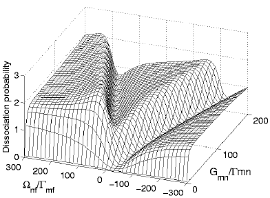
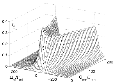
Figure 10: Dissociation probability (a) and population of level $f$ (b) as functions of $\Omega_{nf}/\Gamma_{mf}$ and $G_{mn}/\Gamma_{mn}$. Here, $\gamma_{nn}/\Gamma_{mn}=3$, $\gamma_{ff}/\Gamma_{mf}=3$, $q_{nn}=0.2$, $q_{ff}=-0.5$, $q_{nf}=10$, $w_{n}/\Gamma_{n}=0.1$, $w_{f}=0$, $\Omega_{mn}=0$.

Figure 10 shows that the dissociation rate can be considerably eliminated or alteratively enhanced by varying either the intensity of the splitting field or the detuning $\Omega_{nf}$. The spectral lineshape at constant field intensities has a well-known asymmetrical Fano profile. The plot (b) shows opportunities for manipulating the population of level $f$.

The properties of LICS are essentially determined by the Fano parameters, which indicate an asymmetry in the distribution of the oscillator strength over the continuum, which is illustrated in Fig. 11. By varying the position of the LICS within the continuum, the intensities of the strong laser radiation and the one-photon detuning $\Omega_{1}$, one can manipulate the properties of the laser-induced structures. Large two-photon detunings lead to the vanishing of any interference phenomena in the continuum and thus is equivalent to the field $E_{3}$ being turned off.

(a)                                                     (b)
     

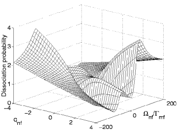
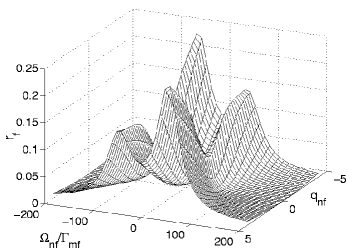
Figure 11: Dissociation probability (a) and population of level $f$ (b) as functions of $\Omega_{nf}/\Gamma_{mf}$ and of the Fano parameter $q_{nf}$. Here, $G_{mn}/\Gamma_{mn}=50$. The other parameters are the same as in the previous figure.

(a)                                                     (b)
     

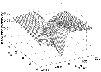
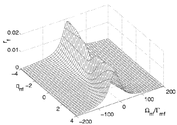
Figure 12: Dissociation probability (a) and population of level $f$ (b) as functions of $\Omega_{nf}/\Gamma_{mf}$ and of the Fano parameter $q_{nf}$. Here, $G_{mn}=0$. The other parameters are the same as in the previous figure.

The above obtained results show that dissociation and population transfer through the continuum can be controlled by the field coupled to the discrete transition. Figure 12 displays a very trivial behavior for $E_{1}$ turned off. Other opportunities of manipulating two-photon dissociation and populations transfer are associated with the control field coupling discrete and continuous states.

In the next subsection, we investigate how such behavior may exhibit itself in difference-frequency four-wave mixing and nonlinear-optical generation of frequency-tunable radiation through the continuous states in folded schemes.

3.2.2 Coherent control of generated radiation in folded schemes

Here we consider the case where the fundamental $E_{1}$ and generated $E_{S}$ fields are weak. Then the solution of the density matrix equations (Section 3.1) for a closed-type scheme takes the form

$$r_{mn}=iG_{mn}y_{mf}/(y_{mn}y_{mf}-b_{1}^{mm}),$$

$$r_{mf}=-iG_{mn}\gamma_{nf}^{m}(1-iq_{nf})/(y_{mn}y_{mf}-b_{1}^{mm}).$$ (3.53)

Similarly, for the case where the field $E_{S}$ is the probe radiation and $E_{1}$ is the generated one, we obtain

$$R_{mf}=iG_{mf}y_{mn}/(y_{mn}y_{mf}-b_{1}^{mm}),$$

$$R_{mn}=iG_{mf}\gamma_{fn}^{m}(1-iq_{fn})/(y_{mn}y_{mf}-b_{1}^{mm}).$$ (3.54)

Then the wave equations for weak fields, coupled by the four-wave mixing process $\omega_{S}\leftrightarrow\omega_{1}-\omega_{2}+\omega_{3}$, have the form

$$dE_{S}(z)/dz ={\rm i}2\pi k_{S}^{\prime}\chi^{(3)}_{S}E_{2}^{*}E_{3}E_{1}(z)\exp({\rm i}\Delta kz),$$

$$dE_{1}(z)/dz ={\rm i}2\pi k_{1}^{\prime}\chi^{(3)}_{1}E_{2}E^{*}_{3}E_{S}(z)\exp(-{\rm i}\Delta kz),$$ (3.55)

where $\Delta k=k_{S}-k_{1}+k_{2}-k_{3}$.

(a)                                                            (b)
     

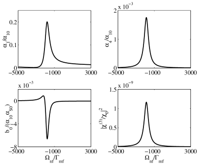
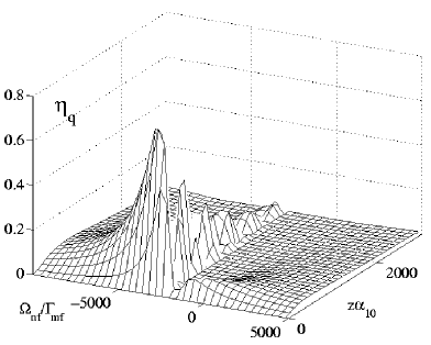
Figure 13: Dependence of the absorption coefficients $\alpha_{1}/\alpha_{10}$ and $\alpha_{S}/\alpha_{10}$, of the conversion rate $b/(\alpha_{10}\alpha_{40})$, and of the squared modulus of the nonlinear susceptibility $|\overline{\chi}^{(3)}|^{2}$, on the detuning $\Omega_{nf}$ (a), and dependence of the quantum conversion efficiency $\eta_{\rm q}$ on the optical thickness and on $\Omega_{nf}$ (b). Here, $C=0.5$, $g_{n}=100$, $g_{f}=6000$, $\Omega_{1}/\Gamma_{mn}=0$, $q_{ff}=-0.5$, $q_{nn}=0.2$, $q_{nf}=0$, (a,b).

Analogously to (2.2), the solution of equations (3.55) can be presented like (2.23) with $\overline{\eta}_{{\rm q}0}=\eta_{{\rm q}0}^{0}|\overline{\chi}^{(3)}|^{2}g_{n}g_{f}$, where $g_{n}=\gamma_{nn}/\Gamma_{mn}$, $g_{f}=\gamma_{ff}/\Gamma_{mf}$. With the aid of the approximate expressions

$$\alpha_{10}=4\pi{\omega_{1}}{|d_{mn}|^{2}/c\hbar\Gamma_{mn}},\>\alpha_{S0}=4\pi{\omega_{S}}|d_{mf}|^{2}/c\hbar\Gamma_{mf},$$

$$|\chi_{0}|^{2}=(\pi/8\hbar^{2})^{2}(1+q_{nf}^{2})|d_{mn}d_{n\varepsilon}d_{\varepsilon f}d_{fm}|^{2}(\Gamma_{mn}\Gamma_{mf})^{-2},$$ (3.56)

we obtain that $\eta_{{\rm q}0}^{0}=(\pi/2)^{2}(1+q_{nf}^{2})$. Other notations are the same as in Section 2.4.

(a)                                                            (b)
     

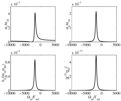
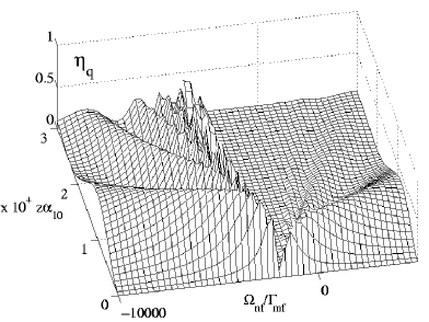
(c)

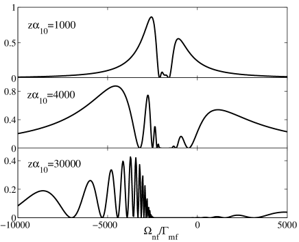
Figure 14: Dependence of the absorption coefficients $\alpha_{1}/\alpha_{10}$ and $\alpha_{S}/\alpha_{10}$, of the conversion rate $b/(\alpha_{10}\alpha_{40})$, and of the squared modulus of the nonlinear susceptibility $|\overline{\chi}^{(3)}|^{2}$ on the detuning $\Omega_{nf}$ (a). Dependence of the quantum conversion efficiency $\eta_{\rm q}$ on $\Omega_{nf}$ for $z\alpha_{10}=10^{3}$; $z\alpha_{10}=4\cdot 10^{3}$; $z\alpha_{10}=3\cdot 10^{4}$ (b). Dependence of the quantum conversion efficiency $\eta_{\rm q}$ on the optical thickness and on $\Omega_{nf}$ (c). Here, $g_{n}=6000$, and the other parameters are the same as in the previous figure.

(a)                                                            (b)
     

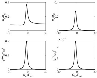
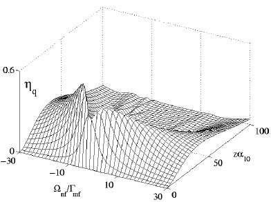
Figure 15: Dependencies of the absorption coefficients $\alpha_{1}/\alpha_{10}$ and $\alpha_{S}/\alpha_{10}$, of the rate of conversion $\overline{b}$, and of the square of the modulus of the nonlinear susceptibility $|\overline{\chi}^{(3)}|^{2}$ on the detuning $\Omega_{nf}$ (a). Dependence of the quantum conversion efficiency $\eta_{\rm q}$ on the optical thickness and on $\Omega_{nf}$ (b). Here, $g_{n}=10$, $g_{f}=6.5$. The other parameters are the same as in the previous figure.

(a)                                                            (b)
     

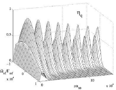
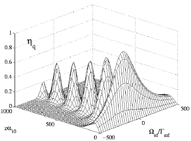
(c)

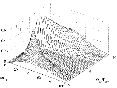
Figure 16: Dependence of the quantum conversion efficiency $\eta_{\rm q}$ on the optical thickness and on $\Omega_{nf}$ for different $q_{nf}$. Here, $g_{n}=10$, $g_{f}=20$; $q_{nf}=100$ (a), $q_{nf}=5$ (b), $q_{nf}=0$ (c). The other parameters are the same as in the previous figure.

(a)                                                            (b)
     

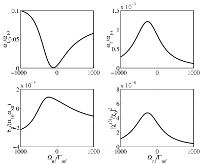
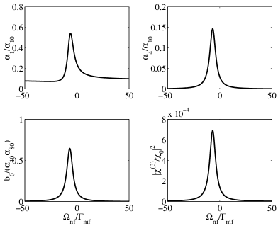
Figure 17: Dependence of the absorption coefficients $\alpha_{1}/\alpha_{10}$ and $\alpha_{S}/\alpha_{10}$, of the rate of conversion $\overline{b}$, and of the squared modulus of the nonlinear susceptibility $|\overline{\chi}^{(3)}|^{2}$ on the detuning $\Omega_{nf}$. Here, $q_{nf}=5$ (a), $q_{nf}=0$ (b). The other parameters are equal to those in Fig. 16.

(a)                                                    (b)
     

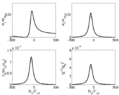
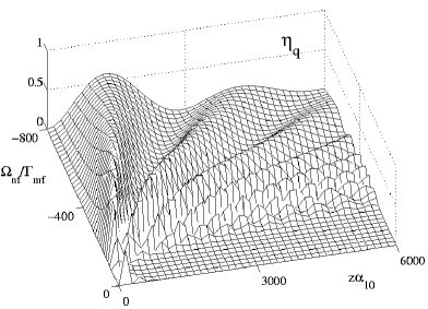
Figure 18: Dependence of the absorption indices $\alpha_{1}/\alpha_{10}$ and $\alpha_{S}/\alpha_{10}$, of the conversion rate $\overline{b}$, and of the squared modulus of the nonlinear susceptibility $|\overline{\chi}^{(3)}|^{2}$ on the detuning $\Omega_{nf}$ (a). Dependence of the quantum conversion efficiency $\eta_{\rm q}$ on the optical thickness and on $\Omega_{nf}$ [$\max(\eta_{q})=0.87$] (b). Here $q_{nf}=5$, $\Omega_{mn}/\Gamma_{mn}=100$. The other parameters are the same as in the previous figure.

Figure 13 illustrates the case where the strong fields are so large that power-broadening exceeds the half-width of the transitions ($\Gamma_{ij}$), and also $g_{f}>>g_{n}$. Then the generation maximum falls to the parameter range for which absorbtion of the fundamental radiation becomes minimum and the rate of conversion is positive. With that, an oscillation regime appears. Within the interval of $\Omega_{nf}/\Gamma_{mf}$ from $-1000$ to $3000$, the rates of absorbtion and generation are almost equal ($b_{0}\approx 0$), and the oscillations reduce to only one maximum of $\eta_{q}$. Figure 14 depicts the case where both driving parameters are equal ($g_{n}=g_{f}=6000$). Here the maximum of $\eta_{q}$ also falls within the range of minimum absorption of the fundamental radiation, and a conversion dip corresponds to the maximum of $\alpha_{1}$. Interference of LICS along with splitting of the discrete resonance give rise to complex structures in $\eta_{q}$ while the waves propagate through the nonlinear medium [see Fig. 14(c)]. For the driving parameters about three order less than in the previous case, and $g_{n}=g_{f}$, the implementation of interference allows one to achieve four orders of increase of the conversion rate $b_{0}$ (Fig. 15). The maximum in $\eta_{q}$ becomes somehow smaller but is reached at a much shorter length of the nonlinear medium. With greater Fano parameters $q_{nf}$, the potential enhancement of the output of generation through manipulating the interplay of LICS becomes greater. As shown in Fig. 16, $\eta_{q}\rightarrow 1$ with $q_{nf}\rightarrow\infty$ provided by the appropriate choice of the control fields intensity. Maxima of the quantum efficiency of conversion process reach $0.996$ for $q_{nf}=100$, $0.919$ for $q_{nf}=5$ and $0.569$ for $q_{nf}=0$. At greater magnitudes of $q_{nf}$, the resonance broadening increases, which leads to the requirement of longer nonlinear medium. This is seen from comparison of Figs. 17(a) and 17(b). It is seen from comparison of Figs. 16(b) and 18(b) that most of the opportunities for manipulation appear at moderate detunings $\Omega_{mn}$.

Conclusions

The technique of quantum control of such processes as ionization, chemical reactivity through dissociation of molecules and population transfer, and four-wave mixing is further developed. Other applications involve discrete and broad-band spectra in solids. The approach is based on manipulating constructive and destructive interference of several quantum pathways involving both discrete energy levels (bound states) and energy continua (free states). Analytical and numerical solutions of the set of coupled density-matrix equations and Maxwell equations for travelling electromagnetic waves are found for the continuous-wave regime.

Novel opportunities are shown for suppression or alternatively enhancement of photophysical processes as well as photochemical processes related with branching chemical reactions. These opportunities are associated with the overlap of two laser-induced continuum structures induced by two control fields, while the third strong field controls a discrete transition. The expressions obtained and numerical models developed are used to demonstrate the feasibility of manipulation of the spectral characteristics of the absorption and dispersion both for discrete transitions and the spectral continua in the presence of additional strong laser radiations. Related opportunities to form laser-induced transparency and to enhance four-wave-mixing nonlinear-optical polarizations are investigated as well. It is shown that the implementation of such nonlinear interference effects makes it possible to utilize the advantages of multiple resonances and strong radiations for considerable improvement of the generation of short-wavelength radiation. Among the important features discovered is the fact that the constructive or destructive nature of interference is governed not only by the ratio of the intensities and by the detunings from the discrete resonances, but also by the composite Fano parameters for transitions between high-lying discrete levels over the continuum states. The results can be generalized to higher-order processes. The matrix elements of the interaction Hamiltonian should then be replaced with the corresponding composite multiphoton matrix elements.

References

• [1] Yu. I. Heller and A. K. Popov, ”Autoionizing-like resonances induced by a laser field,” Opt. Commun. 18, 7-8 (1976).
• [2] Yu. I. Heller and A. K. Popov, ”Parametric generation and absorption of VUV radiation controlled by laser-induced autoionizing-like resonances in continuum,” Opt. Commun. 18, 449-51 (1976).
• [3] Yu. I. Heller, V. F. Lukinykh, A. K. Popov, and V. V. Slabko, ”Experimental evidence for laser-induced autoionizing-like resonances in the continuum,” Phys. Lett. A 82, 4-6 (1981).
• [4] Yu. I. Heller and A. K. Popov, ”Laser-induced narrowing of autoionizing resonances studied by the method of parametric generation,” Phys. Lett. 50 A, 453-4 (1976).
• [5] Yu. I. Heller and A. K. Popov, ”Laser-induced narrowing of autoionizing resonances in multiphoton ionization spectrum,” Opt. Commun. 38, 345-7 (1981).
• [6] Yu. I. Heller and A. K. Popov, ”Narrowing of autoionizing resonances in multiphoton ionization spectra,” Pisma v Zhurnal Tekhnicheskoi Fiziki 7, 719-2 (1981) [Engl.transl.: Letters to the Journal of Technical Physics (JTP Letters)].
• [7] Yu.I. Heller and A.K. Popov, Laser Induction of Nonlinear Resonanses in Continuous Spectra (Novosibirsk, Nauka, 1981) [Engl. transl.: Journ. Sov. Laser Research 6, N 1-2, 1-84s (1985) (Plenum, c/b Consultants Bureau, NY, USA)].
• [8] P.L. Knight, M.A. Lander and B.J. Dalton, ”Laser-induced continuum structure”, Phys. Rep. 190, 1-61 (1990).
• [9] O. Faucher, D. Charalambidis, C. Fotakis, Jian Zhang and P. Lambropoulos, ”Control of laser-induced continuum structure in the vicinity of autoionizing states,” Phys. Rev. Lett. 70, 3004-7 (1993).
• [10] S. Cavaliery, M. Matera, F. S. Pavone, Jian Zhang, P. Lambropoulos and T. Nakajima, ”High-sensitivy study of laser-induced birefrigence and dichrois in the ionization continuum of cesium,” Phys. Rev. A 47, 4219-26 (1993).
• [11] S.J. van Enk, Jiang Zhang and P. Lambropoulos, ”Pump-induced transparency and enhanced third-harmonic generation near an autoionizing state,” Phys. Rev. A 50, 3362-5 (1994).
• [12] S. Cavaliery, R. Eramo and L. Fini, ”Laser-induced structures in the continuum of sodium: A weak dressing field measurement,” J. Phys. B: At. Mol. Opt. Phys. 28, 1739-1801 (1995).
• [13] N.E. Karapanagioti, D. Charalambidis, C. J. G. J. Uiterwaal and C. Fotakis, ”Effects of coherent coupling of autoionizing states on multiphoton ionization,” Phys. Rev. A 53, 2587-97 (1996).
• [14] A. K. Popov, ”Inversionless amplification and laser-induced transparency at discrete transitions and transitions to the continuum,” Bull. Russ. Acad. Sci. (Physics) 60, 927-45 (1996); http://xxx.lanl.gov/abs/quant-ph/0005108.
• [15] S. Cavaliery, R. Eramo and L. Fini, ”Phase-controlled quantum interference in two-color atomic photoionization,” Phys. Rev. A 55, 2941-4 (1997).
• [16] A. K. Popov and V. V. Kimberg, ”Nonlinear-optical generation of short-wavelength radiation controlled by laser-induced interference structures, Quantum Electron. 28, 228-34 (1998) [translated from Kvantovaya Elektronika 25, 236-42 (1998)]; http://turpion.ioc.ac.ru/.
• [17] D. J. Tennor and S. A. Rice, ”Control of selectivity of chemical reaction via control of wave packet evolution,” J. Chem. Phys. 83, 5013-18 (1985).
• [18] M. Shapiro and P. Brumer, ”Laser control of product quantum state populations in unimolecular reactions,” J. Chem. Phys. 84, 4103-04 (1986).
• [19] D. J. Tennor, R. Kosloff and S. A. Rice, ”Coherent pulse sequence induced control of selectivity of reactions – exact quantum-mechanical calculations,” J. Chem. Phys. 85, 5805-20 (1986).
• [20] T. Seideman, M. Shapiro and P. Brumer, ”Coherent radiative control of unimolecular reactions: selective bond breaking with picosecond pulses,” J. Chem. Phys. 90, 7132-6 (1989).
• [21] U. Gaubatz, P. Rudecki, S. Schiemann and K. Bergmann, ”Population transfer between molecular vibrational levels by stimulated Raman scattering with overlapping laser: A new concept and experimental results,” J. Chem. Phys. 92, 5363-76 (1990).
• [22] P. Brumer and M. Shapiro, ”Laser control of molecular processes,” Ann. Rev. Phys. Chem. 43, 257-82 (1992).
• [23] S. Schiemann, A. Kuhn, S. Steuerwald, and K. Bergmann, ”Coherent population transfer in NO with pulsed lasers,” Phys. Rev. Lett. 71, 3637-40 (1993).
• [24] M. V. Danileyko, V. I. Romanenko and L. P. Yatsenko, ”Landau-Zener transition and population tansfer in the three level system driven by two delayed laser pulses,” Opt. Commun. 109, 462-6 (1994).
• [25] M. V. Danileiko, V. I. Romanenko and L. P. Yatsenko ”Adiabatic population transfer on magnetic sublevels of molecules – a new possibility of its motion control,” Ukraine Phys. J. 40, 665-9 (1995).
• [26] B. W. Shore, J. Martin, M. Fewell and K. Bergmann, ”Coherent population transfer in multilevel systems with magnetic sublevels. I. Numerical studies,” Phys. Rev. A 52, 566-82 (1995).
• [27] J. Martin, B. W. Shore and K. Bergmann, ”Coherent population transfer in multilevel systems with magnetic sublevels. II. Algebraic analysis,” Phys. Rev A 52, 583-96 (1995).
• [28] J. Martin , B. W. Shore, and K. Bergmann, ”Coherent population transfer in multilevel systems with magnetic sublevels. III. Experimental results,” Phys. Rev. A 54, 1556-69 (1996).
• [29] T. Halfmann and K. Bergmann, ”Coherent population transfer and dark resonances in sulphur dioxide molecules,” J. Chem. Phys. 104, 7068-82 (1996).
• [30] A. Shnitman, I. Sofer, I. Golub, A. Yogev, M. Shapiro, Z. Chen and P. Brumer, ”Experimental observation of laser control: The Na2 - Na+Na(3d), Na(3p) branching photodissociation reaction,” Phys. Rev. Lett. 76, 2886-89 (1996).
• [31] R. J. Gordon and S. A. Rice, ”Active control of the dynamics of atoms and molecules,” Ann. Rev. Phys. Chem. 48, 601-41 (1997).
• [32] M. Shapiro and P. Brumer, ”Quantum control of chemical reactions”, Trans. Farad. Soc. 93, 1263-77 (1997)
• [33] M. Shapiro, P. Brumer, and Z. Chen, ”Simultaneous control of selectivity and yield of molecular dissociation: pulsed incoherent interference control,” Chem. Phys. 217, 325-40 (1997).
• [34] P. Brumer and M. Shapiro, ”Quantum interference in the control of molecular processes”, Phil. Trans. R. Soc. London A 355, 2409-12 (1997).
• [35] A. Kuhn, S. Steuerwald and K. Bergmann, ”Coherent population transfer in no with pulsed laser: Consequences of hyperfine structure, Doppler broadening and electromagnetically-induced absorption,” Europ. Phys. J. D 1, 57-70 (1998).
• [36] K. Bergmann, H. Theuer and B. W. Shore, ”Coherent population transfer among quantum states of atoms and molecules,” Rev. Mod. Phys. 70, 1003-26 (1998).
• [37] N. V. Vitanov, B. W. Shore, and K. Bergmann, ”adiabatic population transfer in multistate chains via dressed intermediate states,” Europ. Phys. J. D 4, 15-29 (1998).
• [38] M. N. Kobrak and S. A. Rice, ”Equivalence of the Kobrak-Rice photoselective adiabatic passage and the Brumer- Shapiro strong field methods for control of product formation in a reaction,” J. Chem. Phys. 109, 1-10 (1998).
• [39] M. N. Kobrak and S. A. Rice, ”Coherent population transfer via a resonant intermediate state: The breakdown of adiabatic passage,” Phys. Rev. A 57, 1158-63 (1998).
• [40] M. N. Kobrak and S. A. Rice, ”selective photochemistry via adiabatic passage: An extension of stimulated Raman adiabatic passage for degenerate final states,” Phys. Rev. A 57, 2885-94 (1998).
• [41] R. J. Gordon, L. Zhu and T. Seideman, ”Coherent control of chemical reactions,” Acc. Chem. Res. 32, 1007-16 (1999).
• [42] E. Frishman, M. Shapiro and P. Brumer, ”Coherent enhancement and suppression of reactive scattering and tunneling,” J. Chem. Phys. 110, 9-11 (1999).
• [43] M. Shapiro and P. Brumer, ”Coherent control of atomic, molecular and electronic processes,” in Advances in Atomic, Molecular and Optical Physics, Vol. 42, edited by B. Bederson and H. Walther (Academic Press, San Diego, 1999), pp. 287-343.
• [44] I. R. Sola, V. S. Malinovsky, B. Y. Chang, J. Santamaria and K.Bergmann, ”Coherent population transfer in three-level $\Lambda$-Systems by chirped laser pulses: How to minimize the population of the intermediate level,” Phys. Rev. A 59, 4494-4501 (1999).
• [45] D. J. Tannor, R. Kosloff and A. Bartanab, ”Laser cooling of internal degrees of freedom of molecules by dynamically trapped states,” Faraday Discuss. 113, 365-83 (1999).
• [46] S. A. Rice, ”Active control of molecular dynamics: Coherence versus chaos,” J. Stat. Phys. 101, 187-212 (2000).
• [47] S. A. Rice, ”Molecular dynamics: Optical control of reactions,” Nature 403, 496-7 (2000).
• [48] S. A. Rice and M. Zhao, Optical Control of Molecular Dynamics (Wiley, New York, 2000), 438 pages.
• [49] S. Kallush and Y. B. Band, ”Short-pulse chirped adiabatic population transfer in diatomic molecules,” Phys. Rev. A 61, 041401R-1-4 (2000).
• [50] M. Shapiro and P. Brumer, ”On the origin of pulse shaping control of molecular dynamics,” J. Chem. Phys. A 105, 2897-902, (2001).
• [51] V. Kurkal and S. A. Rice, ”Sensitivity of the extended STIRAP method of selective population transfer to coupling to background states,” J. Phys. Chem. B 105, 6488-94 (2001).
• [52] V. Kurkal and S. A. Rice, ”Sequential STIRAP-based control of the HCN-CNH isomerization,” Chem. Phys. Lett. 344, 125-37 (2001).
• [53] N. V. Vitanov, M. Fleischhauer, B. W. Shore and K. Bergmann, ”Coherent manipulation of atoms and molecules by sequential pulses,” in Advances of Atomic, Molecular and Optical Physics, Vol. 46, editid by B. Bederson and H. Walther (Academic Press, San Diego, 2001), pp. 55-190.
• [54] T. Halfmann, L. P. Yatsenko, M. Shapiro, B. W. Shore, and K. Bergmann, ”Population trapping and laser-induced continuum structure in helium: Experiment and theory,” Phys. Rev. A 58, R46-9 (1998) .
• [55] L. P. Yatsenko, T. Halfmann, B. W. Shore and K. Bergmann, ”Photoionization suppression by continuum coherence: Experiment and theory,” Phys.Rev. A 59, 2926-2947 (1999).
• [56] A. Vardi, M. Shapiro and K. Bergmann, ”Complete population transfer to and from a continuum and the radiative association of cold Na atoms to produce translationally cold Na2 molecules in specific vib-rotational states,” Optics Express 4, 91-106 (1999).
• [57] N. P. Makarov, A. K. Popov and V. P. Timofeev, ”Influence of absobtion on resonance four-wave frequency mixing,” Kvantovaya Electron. (Moscow) 15, 757-66 (1988) [Engl. Transl.: Sov. J. Quantum Electron. 18, 483-92 (1988)].
• [58] U. Fano and J. W. Cooper, ”Spectral distribution of atomic osscillator strength,” Rev. Mod. Phys. 40 441-86 (1968).
• [59] T. Ya. Popova, A. K. Popov, S. G. Rautian and R. I. Sokolovskii, ”Nonlinear interference processes in emission, absorption and generation spectra,” Zh. Eksp. Teor. Fiz. 57 (1969) 850-63 [Engl. Transl.: JETP 30 (1970) 466-72] http://xxx.lanl.gov/abs/quant-ph/0005094.
• [60] A.K. Popov, Vvedenie v Nelineinuyu Spektroskopiyu (Nauka, Novosibirsk, 1983).
• [61] A. K. Popov and V. M. Shalaev, ”Elimination of Doppler broadening at coherently driven quantum transitions,” Physical Review A 59, R946-9 (1999).
• [62] A. K. Popov and A. S. Baev, ”Enhanced four-wave mixing via elimination of inhomogeneous broadening by coherent driving of quantum transitions with control fields,” Physical Review A 62, 025801-1-4 (2000).