Continuous variable entanglement by radiation pressure

Abstract

We show that the radiation pressure of an intense optical field impinging on a perfectly reflecting vibrating mirror is able to entangle in a robust way the first two optical sideband modes. Under appropriate conditions, the generated entangled state is of EPR type [A. Einstein, et al., Phys. Rev. 47, 777 (1935)].

Keywords: Mechanical effects of light, Entanglement

1 Introduction

The radiation pressure acting on a movable mirror realizes an optomechanical coupling between the incident optical modes and the various vibrational modes of the mirror. The use of this coupling has been proposed many years ago for the implementation of quantum limited measurements of mechanical forces [1], as the interferometric detection of gravitational-waves [2], or atomic force microscopy [3]. Then optomechanical coupling has been proposed for quantum state engineering: for example, it has been shown that it may lead to nonclassical states of both the radiation field [4, 5], and the motional degree of freedom of the mirror [6].

The appearance of quantum effects in ponderomotive systems, paves the way for using them also for quantum information purposes [7]. In particular, quantum information can be encoded in the continuous quadratures of electromagnetic modes [8], and many quantum communication protocols can be implemented using entangled states of optical fields [9]. A typical example of continuous variable entanglement is represented by the two-mode squeezed states at the output of a nondegenerate parametric amplifier [10]. However, it has been showed in Refs. [11, 12, 13] that radiation pressure can also be used to entangle two or more modes of a cavity with a movable and perfectly reflecting mirror. In the present paper, we get rid of the cavity and we show that radiation pressure provides a new way to entangle travelling electromagnetic modes. We shall consider the very simple case of an intense optical mode, incident on a single, vibrating, and perfectly reflecting mirror. A vibrational mode of the mirror will induce sideband modes on the reflected field, which will be shown to be entangled. Entanglement proves to be very robust with respect to the thermal noise acting on the mirror. In particular, for a well defined interaction time, i.e., a given time duration of the incident field, the two first sideband modes become an EPR-correlated pair, identical to the two-mode squeezed state, with the ratio between the optical and the mechanical frequency playing the role of the squeezing parameter.

The paper is organized as follows. In Section II we shall derive the effective Hamiltonian of the system. In Section III we shall exactly solve the dynamics and provide a complete characterization of the reduced state of the system composed by the two reflected sideband modes. Section IV is for concluding remarks.

2 Effective Hamiltonian of the system

Let us consider a perfectly reflecting mirror and an intense laser beam impinging on its surface (see Fig. 1). For simplicity we consider only the motion and the elastic deformations of the mirror taking place along the spatial direction $x$, orthogonal to its reflecting surface.

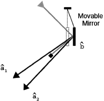
Figure 1: Schematic description of the system. A laser field at frequency $\omega_{0}$ impinges on the mirror oscillating at frequency $\Omega$. In the reflected field two sideband modes are excited at frequencies $\omega_{1}=\omega_{0}-\Omega$ and $\omega_{2}=\omega_{0}+\Omega$.

The electromagnetic field exerts a force on the mirror proportional to its intensity and, at the same time, it is phase-shifted by the mirror displacement from the equilibrium position [14, 15]. In the limit of small mirror displacements, and in the interaction picture with respect to the free Hamiltonian of the electromagnetic field and the mirror displacement field ${\hat{x}({\bf r},t)}$ (${\bf r}$ is the coordinate on the mirror surface), one has the following Hamiltonian [16]

$${\hat{H}} = -\int\,d^{2}{\bf r}\,{\hat{P}}({\bf r},t){\hat{x}}({\bf r},t)\,,$$ (1)

where ${\hat{P}({\bf r},t)}$ is the radiation pressure force [14]. All the continuum of electromagnetic modes with positive longitudinal wave vector $q$ and transverse wave vector ${\bf k}$ contributes to the radiation pressure force. Following Ref.[14], and considering linearly polarized radiation with the electric field parallel to the mirror surface, we have

$${\hat{P}}({\bf r},t) = -\frac{\hbar}{8\pi^{3}}\int d{\bf k}\int dq\int d{\bf k^{\prime}}\int dq^{\prime}\frac{c^{2}qq^{\prime}}{\sqrt{\omega\omega^{\prime}}}({\bf u}_{k}\cdot{\bf u}_{k^{\prime}}){\bf u}_{q}$$ (2)

$$\times \left\{{\hat{a}}({\bf k},q){\hat{a}}({\bf k}^{\prime},q^{\prime})\exp[-i(\omega+\omega^{\prime})t+i({\bf k}+{\bf k}^{\prime})\cdot{\bf r}]\right.$$

$$\left.+{\hat{a}}^{{\dagger}}({\bf k},q){\hat{a}}^{{\dagger}}({\bf k}^{\prime},q^{\prime})\exp[i(\omega+\omega^{\prime})t-i({\bf k}+{\bf k}^{\prime})\cdot{\bf r}]\right.$$

$$\left.+{\hat{a}}({\bf k},q){\hat{a}}^{{\dagger}}({\bf k}^{\prime},q^{\prime})\exp[-i(\omega-\omega^{\prime})t+i({\bf k}-{\bf k}^{\prime})\cdot{\bf r}]\right.$$

$$\left.+{\hat{a}}^{{\dagger}}({\bf k},q){\hat{a}}({\bf k}^{\prime},q^{\prime})\exp[i(\omega-\omega^{\prime})t-i({\bf k}-{\bf k}^{\prime})\cdot{\bf r}]\right\}\,,$$

where ${\hat{a}}({\bf k},q)$ are continuous mode destruction operators obeying the commutation relations

$$\left[{\hat{a}}({\bf k},q),{\hat{a}}^{\dagger}({\bf k}^{\prime},q^{\prime})\right]=\delta({\bf k}-{\bf k}^{\prime})\delta(q-q^{\prime})\,.$$ (3)

Furthermore, the electromagnetic wave frequencies $\omega$ and $\omega^{\prime}$ are given by $\omega=\sqrt{c^{2}(k^{2}+q^{2})}$ and $\omega^{\prime}=\sqrt{c^{2}(k^{\prime 2}+q^{\prime 2})}$ ($c$ is the light speed in vacuum), and ${\bf u}_{k}$, ${\bf u}_{q}$ denote dimensionless unit vectors parallel to ${\bf k}$, $q$ respectively.

The mirror displacement ${\hat{x}({\bf r},t)}$ is generally given by a superposition of many acoustic modes [16]; however, a single vibrational mode description can be adopted whenever detection is limited to a frequency bandwidth including a single mechanical resonance. In particular, focused light beams are able to excite Gaussian acoustic modes, in which only a small portion of the mirror, localized at its center, vibrates. These modes have a small waist $w$, a large mechanical quality factor $Q$, a small effective mass $M$ [16], and the simplest choice is to choose the fundamental Gaussian mode with frequency $\Omega$ and annihilation operator ${\hat{b}}$, with $\left[{\hat{b}},{\hat{b}}^{\dagger}\right]=1$,

$${\hat{x}}({\bf r},t)=\sqrt{\frac{\hbar}{2M\Omega}}\left[{\hat{b}}e^{-i\Omega t}+{\hat{b}}^{{\dagger}}e^{i\Omega t}\right]\exp(-r^{2}/w^{2})\,.$$ (4)

By inserting Eqs. (2) and (4) in Eq. (1) and integrating over the variable ${\bf r}$, one obtains

$${\hat{H}} = -\frac{\hbar w^{2}}{8\pi^{2}}\sqrt{\frac{\hbar}{2M\Omega}}\int d{\bf k}\int dq\int d{\bf k^{\prime}}\int dq^{\prime}\frac{c^{2}qq^{\prime}}{\sqrt{\omega\omega^{\prime}}}({\bf u}_{k}\cdot{\bf u}_{k^{\prime}}){\bf u}_{q}$$ (5)

$$\times \left\{{\hat{a}}({\bf k},q){\hat{a}}({\bf k}^{\prime},q^{\prime})\exp[-i(\omega+\omega^{\prime})t-({\bf k}+{\bf k}^{\prime})^{2}w^{2}/4]\right.$$

$$\left.+{\hat{a}}^{{\dagger}}({\bf k},q){\hat{a}}^{{\dagger}}({\bf k}^{\prime},q^{\prime})\exp[i(\omega+\omega^{\prime})t-({\bf k}+{\bf k}^{\prime})^{2}w^{2}/4]\right.$$

$$\left.+{\hat{a}}({\bf k},q){\hat{a}}^{{\dagger}}({\bf k}^{\prime},q^{\prime})\exp[-i(\omega-\omega^{\prime})t-({\bf k}-{\bf k}^{\prime})^{2}w^{2}/4]\right.$$

$$\left.+{\hat{a}}^{{\dagger}}({\bf k},q){\hat{a}}({\bf k}^{\prime},q^{\prime})\exp[i(\omega-\omega^{\prime})t-({\bf k}-{\bf k}^{\prime})^{2}w^{2}/4]\right\}$$

$$\times\left\{{\hat{b}}e^{-i\Omega t}+{\hat{b}}^{{\dagger}}e^{i\Omega t}\right\}\,.$$

In common situations, the acoustical waist $w$ is much larger than typical optical wavelengths [16], and therefore we can approximate $\exp\left\{-({\bf k}\pm{\bf k^{\prime}})^{2}w^{2}/4\right\}w^{2}/4\pi\simeq\delta({\bf k}\pm{\bf k^{\prime}})$ and then integrate Eq. (5) over ${\bf k^{\prime}}$, obtaining

$${\hat{H}} = -\frac{\hbar}{2\pi}\sqrt{\frac{\hbar}{2M\Omega}}\int d{\bf k}\int dq\int dq^{\prime}\frac{c^{2}qq^{\prime}}{\sqrt{\omega\omega^{\prime}}}$$ (6)

$$\times \left\{-{\hat{a}}({\bf k},q){\hat{a}}(-{\bf k},q^{\prime})\exp[-i(\omega+\omega^{\prime})t]\right.$$

$$\left.-{\hat{a}}^{{\dagger}}({\bf k},q){\hat{a}}^{{\dagger}}(-{\bf k},q^{\prime})\exp[i(\omega+\omega^{\prime})t]\right.$$

$$\left.+{\hat{a}}({\bf k},q){\hat{a}}^{{\dagger}}({\bf k},q^{\prime})\exp[-i(\omega-\omega^{\prime})t]\right.$$

$$\left.+{\hat{a}}^{{\dagger}}({\bf k},q){\hat{a}}({\bf k},q^{\prime})\exp[i(\omega-\omega^{\prime})t]\right\}\times\left\{{\hat{b}}e^{-i\Omega t}+{\hat{b}}^{{\dagger}}e^{i\Omega t}\right\}\,.$$

We now make the Rotating Wave Approximation (RWA), that is, we neglect all the terms oscillating in time faster than the mechanical frequency $\Omega$. This means averaging the Hamiltonian over a time $\tau$ such that $\Omega\tau\gg 1$, yielding the following replacements in Eq. (6)

$$\exp\left\{\pm i(\omega^{\prime}\pm\omega\pm\Omega)t\right\}\rightarrow\frac{2\pi}{\tau}\delta(\omega^{\prime}\pm\omega\pm\Omega).$$ (7)

The parameter $\tau$ is not arbitrary, but its inverse, $1/\tau=\Delta\nu_{det}$, is the detection bandwidth, that is, the spectral resolution of the detection apparatus employed.

Since $\omega$ and $\omega^{\prime}$ are positive and $\Omega$ is much smaller than typical optical frequencies, the two terms $\delta(\omega^{\prime}+\omega\pm\Omega)$ give no contribution, while the other two terms can be rewritten as

$$\frac{2\pi}{\tau}\delta(\omega^{\prime}-\omega\pm\Omega)=2\pi\Delta\nu_{det}\delta(q^{\prime}-\bar{q}_{\pm})\frac{\omega^{\prime}(\bar{q}_{\pm})}{c^{2}\bar{q}_{\pm}},$$ (8)

where $\bar{q}_{\pm}=\sqrt{(\omega\pm\Omega)^{2}/c^{2}-k^{2}}$. Integrating over $q^{\prime}$ we get

$${\hat{H}} = -\hbar\Delta\nu_{det}\sqrt{\frac{\hbar}{2M\Omega}}\int d{\bf k}\int dq\frac{q}{\sqrt{\omega}}\left\{{\hat{a}}({\bf k},q){\hat{a}}^{{\dagger}}\left({\bf k},\bar{q}_{+}\right){\hat{b}}\;\sqrt{\omega+\Omega}\right.$$ (9)

$$\left.+{\hat{a}}({\bf k},q){\hat{a}}^{{\dagger}}\left({\bf k},\bar{q}_{-}\right){\hat{b}}^{{\dagger}}\sqrt{\omega-\Omega}\right.$$

$$\left.+{\hat{a}}^{{\dagger}}({\bf k},q){\hat{a}}\left({\bf k},\bar{q}_{+}\right){\hat{b}}^{{\dagger}}\sqrt{\omega+\Omega}\right.$$

$$\left.+{\hat{a}}^{{\dagger}}({\bf k},q){\hat{a}}\left({\bf k},\bar{q}_{-}\right){\hat{b}}\sqrt{\omega-\Omega}\right\}\,,$$

where we have used the fact that $\omega^{\prime}(\bar{q}_{\pm})=\omega\pm\Omega$.

We now consider the situation where the radiation field incident on the mirror is characterized by an intense, quasi-monochromatic, laser field with transversal wave vector ${\bf k_{0}}$, longitudinal wave vector $q_{0}$, cross-sectional area $A$, and power ${\wp}$. Since this component is very intense, it can be treated as classical and one can approximate ${\hat{a}}({\bf k},q)\simeq\alpha({\bf k},q)$ in Eq. (9), where (with an appropriate choice of phases)

$$\alpha({\bf k},q)=-i\sqrt{\frac{(2\pi)^{3}{\wp}}{\hbar\omega_{0}cA}}\delta({\bf k}-{\bf k_{0}})\delta(q-q_{0})\,,$$ (10)

with $\omega_{0}=c\sqrt{{\bf k_{0}}^{2}+q_{0}^{2}}$.

Due to the Dirac delta, the only nonvanishing terms in the optomechanical interaction driven by the intense laser beam involve only two back-scattered waves, that is, the sidebands of the driving beam at frequencies $\omega_{0}\pm\Omega$, as described by

$${\hat{H}} = i\hbar\Delta\nu_{det}\sqrt{\frac{\hbar}{2M\Omega}}q_{0}\sqrt{\frac{{\wp}}{\hbar\omega_{0}cA}}$$ (11)

$$\times \left\{\sqrt{\frac{\omega_{0}+\Omega}{\omega_{0}}}{\hat{a}}^{{\dagger}}\left({\bf k_{0}},\bar{q}_{+}\right){\hat{b}}+\sqrt{\frac{\omega_{0}-\Omega}{\omega_{0}}}{\hat{a}}^{{\dagger}}\left({\bf k_{0}},\bar{q}_{-}\right){\hat{b}}^{\dagger}\right.$$

$$\left.-\sqrt{\frac{\omega_{0}+\Omega}{\omega_{0}}}{\hat{a}}\left({\bf k_{0}},\bar{q}_{+}\right){\hat{b}}^{\dagger}-\sqrt{\frac{\omega_{0}-\Omega}{\omega_{0}}}{\hat{a}}\left({\bf k_{0}},\bar{q}_{-}\right){\hat{b}}\right\},$$

where now $\bar{q}_{\pm}=\sqrt{(\omega_{0}\pm\Omega)^{2}/c^{2}-k_{0}^{2}}$. The physical process described by this interaction Hamiltonian is very similar to a stimulated Brillouin scattering [17], even though in this case the Stokes and anti-Stokes component are back-scattered by the acoustic waves at reflection, and the optomechanical coupling is provided by the radiation pressure and not by the dielectric properties of the mirror.

In practice, either the driving laser beam and the back-scattered modes are never monochromatic, but have a nonzero bandwidth. In general the bandwidth of the back-scattered modes is determined by the bandwidth of the driving laser beam and that of the acoustic mode. However, due to its high mechanical quality factor, the spectral width of the mechanical resonance is negligible (about $1$ Hz) and, in practice, the bandwidth of the two sideband modes $\Delta\nu_{mode}$ coincides with that of the incident laser beam. It is then convenient to consider this nonzero bandwidth to redefine the bosonic operators of the Stokes and anti-Stokes modes to make them dimensionless,

$${\hat{a}}_{1} = 2\pi\sqrt{\frac{2\pi\Delta\nu_{mode}}{cA}}{\hat{a}}\left({\bf k_{0}},\bar{q}_{-}\right)=2\pi\sqrt{\frac{\Delta q}{A}}{\hat{a}}\left({\bf k_{0}},\bar{q}_{-}\right)$$ (12)

$${\hat{a}}_{2} = 2\pi\sqrt{\frac{2\pi\Delta\nu_{mode}}{cA}}{\hat{a}}\left({\bf k_{0}},\bar{q}_{+}\right)=2\pi\sqrt{\frac{\Delta q}{A}}{\hat{a}}\left({\bf k_{0}},\bar{q}_{+}\right),$$ (13)

so that Eq.(11) reduces to an effective Hamiltonian

$${\hat{H}}_{eff}=-i\hbar\chi({\hat{a}}_{1}{\hat{b}}-{\hat{a}}^{{\dagger}}_{1}{\hat{b}}^{{\dagger}})-i\hbar\theta({\hat{a}}_{2}{\hat{b}}^{{\dagger}}-{\hat{a}}^{{\dagger}}_{2}{\hat{b}})\,,$$ (14)

where the couplings $\chi$ and $\theta$ are given by

$$\chi = q_{0}\Delta\nu_{det}\sqrt{\frac{\hbar}{2M\Omega}}\sqrt{\frac{{\wp}}{\Delta\nu_{mode}\hbar\omega_{0}}}\sqrt{\frac{\omega_{0}-\Omega}{\omega_{0}}}$$ (15)

$$= \cos\phi_{0}\sqrt{\frac{{\wp}\Delta\nu_{det}^{2}(\omega_{0}-\Omega)}{2M\Omega c^{2}\Delta\nu_{mode}}}$$

$$\theta = \chi\sqrt{\frac{\omega_{0}+\Omega}{\omega_{0}-\Omega}},$$ (16)

with $\phi_{0}=\arccos(cq_{0}/\omega_{0})$, is the angle of incidence of the driving beam. It is possible to verify that with the above definitions, the Stokes and anti-Stokes annihilation operators $a_{1}$ and $a_{2}$ satisfy the usual commutation relations $\left[a_{i},a_{j}^{\dagger}\right]=\delta_{i,j}$.

3 System dynamics

Eq. (14) contains two interaction terms: the first one, between modes ${\hat{a}}_{1}$ and ${\hat{b}}$, is a parametric-type interaction leading to squeezing in phase space [10], and it is able to generate the EPR-like entangled state which has been used in the continuous variable teleportation experiment of Ref. [18]. The second interaction term, between modes ${\hat{a}}_{2}$ and ${\hat{b}}$, is a beam-splitter-type interaction [10], which may degrade the entanglement between modes ${\hat{a}}_{1}$ and ${\hat{b}}$ generated by the first term. In general, one has a system of three bosonic modes, coupled by a bilinear interaction. The corresponding Hamiltonian evolution of the system can be straightforwardly obtained. This Hamiltonian description satisfactorily reproduces the dynamics as long as the dissipative coupling of the mirror vibrational mode with its environment is negligible. This happens in the case of modes with a high-Q mechanical quality factor. In this case, the mechanical frequency $\Omega$ is sufficiently high (some MHz) so that the RWA of Eq. (7) can be made, and at the same time we can consider an interaction time, i.e., a time duration of the incident laser pulse, much smaller than the relaxation time of the vibrational mode (which can be of order of one second).

The system dynamics can be easily studied through the (normally ordered) characteristic function $\Phi(\mu,\nu,\zeta)$, where $\mu,\nu,\zeta$ are the complex variables corresponding to the operators ${\hat{a}}_{1},{\hat{b}},{\hat{a}}_{2}$ respectively. From the Hamiltonian (14) the dynamical equation for $\Phi$ results

$${\dot{\Phi}} = \chi\left(\mu\nu+\mu^{*}\nu^{*}-\mu^{*}\frac{\partial}{\partial\nu}-\mu\frac{\partial}{\partial\nu^{*}}-\nu^{*}\frac{\partial}{\partial\mu}-\nu\frac{\partial}{\partial\mu^{*}}\right)\Phi$$ (17)

$$+\theta\left(\zeta^{*}\frac{\partial}{\partial\nu^{*}}+\zeta\frac{\partial}{\partial\nu}-\nu^{*}\frac{\partial}{\partial\zeta^{*}}-\nu\frac{\partial}{\partial\zeta}\right)\Phi\,,$$

with the initial condition

$$\Phi(t=0)=\exp\left[-\overline{n}|\nu|^{2}\right]\,,$$ (18)

corresponding to the vacuum for modes ${\hat{a}}_{1}$, ${\hat{a}}_{2}$ and to a thermal state for mode ${\hat{b}}$. The latter is characterized by an average number of excitations $\overline{n}=[\exp(\hbar\Omega/k_{B}T)-1]^{-1}$, $T$ being the equilibrium temperature and $k_{B}$ the Boltzmann constant. Since the initial condition is a Gaussian state of the three-mode system, and the system is linear, the joint state of the whole system at time $t$ is still Gaussian, with characteristic function

$$\Phi = \exp\left[-{\cal A}|\mu|^{2}-{\cal B}|\nu|^{2}-{\cal E}|\zeta|^{2}\right.$$ (19)

$$\left.+{\cal C}\mu\nu+{\cal C}\mu^{*}\nu^{*}+{\cal F}\mu\zeta+{\cal F}\mu^{*}\zeta^{*}+{\cal D}\nu\zeta^{*}+{\cal D}\nu^{*}\zeta\right]\,,$$

where

$${\cal A}(t) = \frac{1}{2(r^{2}-1)^{2}}\left\{\left[1-\cos\left(2\Theta t\right)\right]\left[\overline{n}(r^{2}-1)-1\right]\right.$$ (20)

$$\left.+4r^{2}\left[1-\cos\left(\Theta t\right)\right]\right\}\,,$$

$${\cal B}(t) = \frac{1}{2(r^{2}-1)}\left\{\left[1+\cos\left(2\Theta t\right)\right]\overline{n}(r^{2}-1)+1-\cos\left(2\Theta t\right)\right\}\,,$$ (21)

$${\cal C}(t) = \frac{1}{2(r^{2}-1)^{3/2}}\left\{2r^{2}\sin\left(\Theta t\right)\right.$$ (22)

$$\left.+\left[\overline{n}(r^{2}-1)-1\right]\sin\left(2\Theta t\right)\right\}\,,$$

$${\cal D}(t) = \frac{-r}{2(r^{2}-1)^{3/2}}\left\{\sin\left(\Theta t\right)+\left[\overline{n}(r^{2}-1)-1\right]\sin\left(2\Theta t\right)\right\}\,,$$ (23)

$${\cal E}(t) = \frac{r^{2}}{2(r^{2}-1)^{2}}\left\{\left[1-\cos\left(2\Theta t\right)\right]\left[\overline{n}(r^{2}-1)-1\right]\right.$$ (24)

$$\left.+4\left[1-\cos\left(\Theta t\right)\right]\right\}\,,$$

$${\cal F}(t) = \frac{r}{2(r^{2}-1)^{2}}\left\{\left[1-\cos\left(2\Theta t\right)\right]\left[\overline{n}(r^{2}-1)-1\right]\right.$$ (25)

$$\left.+2(1+r^{2})\left[1-\cos\left(\Theta t\right)\right]\right\}\,,$$

$r=\theta/\chi=\left[(\omega_{0}+\Omega)/(\omega_{0}-\Omega)\right]^{1/2}$ and $\Theta=\chi(r^{2}-1)^{1/2}$. The corresponding density operator can be expressed as

$${\hat{\rho}}_{1b2}=\int\frac{d^{2}\mu}{\pi}\int\frac{d^{2}\nu}{\pi}\int\frac{d^{2}\zeta}{\pi} \Phi(\mu,\nu,\zeta,t)e^{-|\mu|^{2}-|\nu|^{2}-|\zeta|^{2}}$$ (26)

$$\times{\hat{D}}_{1}(-\mu){\hat{D}}_{b}(-\nu){\hat{D}}_{2}(-\zeta)\,,$$

where ${\hat{D}}_{i}$ indicates the corresponding normally ordered displacement operator [19].

Here we are interested in the reduced state of the system composed by the two reflected optical sideband modes. They do not interact directly but their interaction is mediated by the optomechanical coupling of each mode with the moving mirror. This reduced state can be immediately obtained by tracing over the mirror mode ${\hat{b}}$, obtaining

$$\Phi_{12}(\mu,\zeta)=\exp\left[-{\cal A}|\mu|^{2}-{\cal E}|\zeta|^{2}+{\cal F}\left(\mu\zeta+\mu^{*}\zeta^{*}\right)\right]\,.$$ (27)

Introducing the vector of field quadratures ${\hat{\bf v}}=({\hat{X}}_{1},{\hat{P}}_{1},{\hat{X}}_{2},{\hat{P}}_{2})$, where

$${\hat{X}}_{j}=\frac{{\hat{a}}_{j}+{\hat{a}}_{j}^{{\dagger}}}{\sqrt{2}}\,,\quad{\hat{P}}_{j}=\frac{{\hat{a}}_{j}-{\hat{a}}_{j}^{{\dagger}}}{i\sqrt{2}}\,,\quad{j=1,2}\;,$$ (28)

it is possible to connect the characteristic function (27) with the correlation matrix $\Gamma$ of the two sideband modes, defined as $\Gamma_{i,j}=\langle{\hat{\bf v}}_{i}{\hat{\bf v}}_{j}+{\hat{\bf v}}_{j}{\hat{\bf v}}_{i}\rangle/2-\langle{\hat{\bf v}}_{i}\rangle\langle{\hat{\bf v}}_{j}\rangle$, and which, in this case, is equal to

$$\Gamma=\left(\begin{array}[]{cccc}{\cal A}+\frac{1}{2}&0&{\cal F}&0\\ 0&{\cal A}+\frac{1}{2}&0&-{\cal F}\\ {\cal F}&0&{\cal E}+\frac{1}{2}&0\\ 0&-{\cal F}&0&{\cal E}+\frac{1}{2}\end{array}\right)\,.$$ (29)

The Gaussian state of the two optical modes is completely characterized by this correlation matrix. In particular we can employ the necessary and sufficient criterion for entanglement in the case of Gaussian states derived by Simon [20], which allows us to determine the parameter region where the two modes are entangled by the optomechanical interaction with the mirror vibrational mode. Simon’s necessary and sufficient criterion for entanglement becomes, for the two-sideband modes state considered here,

$${\cal T} \equiv \left({\cal A}{\cal E}+\frac{1}{4}+\frac{{\cal A}+{\cal E}}{2}-{\cal F}^{2}\right)^{2}+\frac{1}{16}-\frac{{\cal F}^{2}}{2}$$ (30)

$$-\left(\frac{{\cal A}}{2}+\frac{1}{4}\right)^{2}-\left(\frac{{\cal E}}{2}+\frac{1}{4}\right)^{2}<0$$

As it can be immediately seen from Eqs. (20)-(25), the dynamics of the system is determined only by three dimensionless parameters, $\Theta t$, $r$, and $\overline{n}$, and it is periodic in $\Theta t$ with period $2\pi$. The parameter $r$ is determined by the ratio between the mechanical and the driving laser frequency, $\Omega/\omega_{0}$ and it is always very close to $1$. For this reason in Fig. 2 we show the marker of entanglement ${\cal T}$ as a function of the scaled time $\Theta t$ for $0\leq\Theta t\leq 2\pi$, for different values of the initial mean thermal vibrational number $\overline{n}$ and at a fixed value of $r$, i.e., $r-1=2.5\times 10^{-7}$. Fig. 2 clearly shows that the two sideband modes are almost always entangled (obviously except for $t=2k\pi$, for integer $k$, due to the factorized initial condition) and that this entanglement is extremely robust with respect to the thermal noise acting on the mirror. In fact, the marker of entanglement ${\cal T}$ remains always negative, even at extremely large values of $\overline{n}$. Fig. 2 shows ${\cal T}$ for $\overline{n}=0$ (full line), $\overline{n}=10^{5}$ (dashed line, almost coinciding with that for $\overline{n}=0$), $\overline{n}=5\times 10^{6}$ (dotted-dashed line), and $\overline{n}=10^{7}$ (dotted line). This result is extremely interesting because it shows that radiation pressure proves to be an efficient source of entangled travelling optical fields, not particularly affected by thermal noise. In this treatment we have only considered this kind of noise and we have neglected other more technical noise sources, such as the fluctuations of the intensity and the frequency of the incident driving field. In fact, the latter, differently from thermal noise, are negligible in today experiments involving optomechanical systems [21].

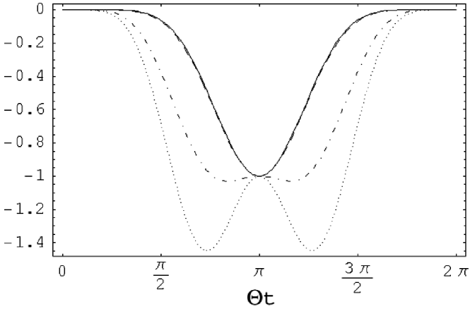
Figure 2: The marker of entanglement ${\cal T}(\Theta t)/|{\cal T}(\pi)|$ vs the scaled time $\Theta t$. The values of other parameters are: $r=1+2.5\times 10^{-7}$ and $\overline{n}=0$ solid line, $\overline{n}=10^{5}$ dashed line, $\overline{n}=5\times 10^{6}$ dashed-dotted line, $\overline{n}=10^{7}$ dotted line.

From Fig. 2, it is evident that ${\cal T}$ at exactly half period, $\Theta t=\pi$, is unaffected by thermal noise, i.e., it is independent of $\overline{n}$. In fact, using Eqs (20)-(25) and (30), it is easy to see that ${\cal T}(\Theta t=\pi)=-4(r+r^{3})^{2}/(r^{2}-1)^{4}$ (actually ${\cal T}$ has been scaled exactly by the modulus of this value in Fig. 2). This independence of $\overline{n}$ is a manifestation of quantum interference between the dynamical effects of the two interaction terms in Eq. (14). It is therefore interesting to see the reduced state of the two reflected sideband modes just at this interaction time, $\Theta t=\pi$. Using Eqs. (20)-(25), one has the following correlation matrix

$$\Gamma(\Theta t=\pi)=$$ (31)

$$=\left(\begin{array}[]{cccc}\frac{4r^{2}}{(r^{2}-1)^{2}}+\frac{1}{2}&0&\frac{2r(1+r^{2})}{(r^{2}-1)^{2}}&0\\ 0&\frac{4r^{2}}{(r^{2}-1)^{2}}+\frac{1}{2}&0&-\frac{2r(1+r^{2})}{(r^{2}-1)^{2}}\\ \frac{2r(1+r^{2})}{(r^{2}-1)^{2}}&0&\frac{4r^{2}}{(r^{2}-1)^{2}}+\frac{1}{2}&0\\ 0&-\frac{2r(1+r^{2})}{(r^{2}-1)^{2}}&0&\frac{4r^{2}}{(r^{2}-1)^{2}}+\frac{1}{2}\end{array}\right)\,.$$ (36)

It is easy to check that this is just the correlation matrix of an EPR-like entangled state, i.e., identical to the two-mode squeezed state generated by a parametric amplifier [10]. The correspondence between the squeezing parameter $\xi$ and our parameters is $\sinh\xi\leftrightarrow 2r(1+r^{2})/(r^{2}-1)^{2}$, so that, in practice one can reach very high two-mode squeezing by choosing $r-1\rightarrow 0$, i.e., by decreasing the ratio $\Omega/\omega_{0}$. This fact can be equivalently seen by evaluating the variances of the linear combination of field quadratures, typical of the two-mode squeezed state, i.e.,

$$\Delta_{-} = \langle(X_{1}-X_{2})^{2}\rangle=\langle(P_{1}+P_{2})^{2}\rangle\,,$$ (37)

$$\Delta_{+} = \langle(X_{1}+X_{2})^{2}\rangle=\langle(P_{1}-P_{2})^{2}\rangle\,.$$ (38)

For $\Theta t=\pi$, one has

$$\Delta_{-}(\Theta t=\pi) = \left(\frac{r-1}{r+1}\right)^{2}\,,$$ (39)

$$\Delta_{+}(\Theta t=\pi) = \left(\frac{r+1}{r-1}\right)^{2}\,.$$ (40)

The time behavior of the variances (37) and (38) is depicted in Fig. 3. It is worth noticing that the typical EPR correlations are available for a wide time range around $\Theta t=\pi$. Furthermore, they are robust against thermal noise since the curves are shown for ${\overline{n}}=10^{5}$, and they practically coincide with those for ${\overline{n}}=0$. That is in agreement with the results shown in Fig.2.

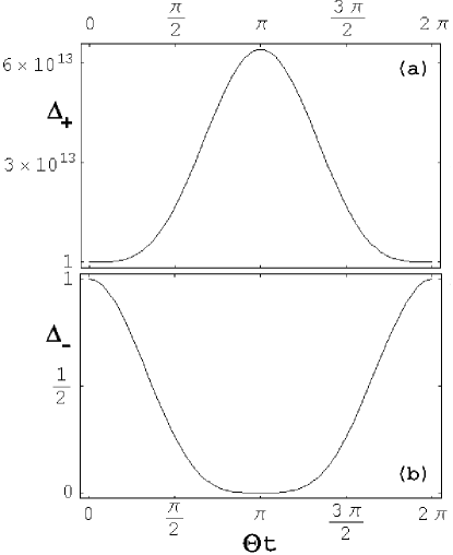
Figure 3: The quantities $\Delta_{+}(\Theta t)$ (a) and $\Delta_{-}(\Theta t)$ (b) are plotted vs the scaled time $\Theta t$. The values of other parameters are $r=1+2.5\times 10^{-7}$ and $\overline{n}=10^{5}$.

4 Results and Conclusions

In conclusion, we have seen that, under appropriate conditions, the radiation pressure of an intense optical pulse impinging on a perfectly reflecting mirror couples efficiently the first two sideband modes induced by a vibrational mode of the mirror. This optomechanical interaction actually entangles the two modes, and quite surprisingly, the resulting entanglement is extremely robust with respect to the thermal noise acting on the mirror. In particular, due to quantum interference, if the interaction time, i.e., the duration of the incident driving pulse, is appropriately tailored, the reduced state of the reflected sideband modes is a two-mode squeezed state. Therefore, rather unexpectedly, radiation pressure could be employed as a new source of entangled two-mode squeezed state, in which the role of the squeezing parameter is played by the ratio between the optical and the mechanical frequency $\omega_{0}/\Omega$. These interesting results hold if the time duration of the pulse satisfies two conditions: i) it has to be much longer than the period of mechanical oscillations, because we have to average over these oscillations; ii) it has to be shorter than the vibrational mode relaxation time (mechanical damping has been neglected in our treatment). These conditions are not extremely easy but they could be realized using micro-opto-electro-mechanical-systems (MOEMS) for example [22]. Possible values are: damping rates $\gamma_{m}\simeq 1$ Hz, ${\wp}=10$W, $\omega_{0}\sim 2\times 10^{15}$ Hz, $\Omega\sim 5\times 10^{8}$ Hz, $\Delta\nu_{det}\sim 10^{7}$ Hz, $\Delta\nu_{mode}\sim t^{-1}\sim 10^{3}$ Hz, and $M\sim 10^{-10}$ Kg, yielding $\chi\simeq\theta\simeq 5\times 10^{5}$ Hz, and $\Theta\simeq 10^{3}$ Hz. Therefore, using well tailored and long pulses (order of $1$ ms), one could realize this new source of two mode squeezing.

References

References

[1]
V. B. Braginsky and F. Y. Khalili,
Quantum Measurement,
(Cambridge University Press, Cambridge, 1992).
[2]
A. Abramovici, et al.,
Science 256, 325 (1992).
[3]
D. Rugar and P. Hansma, Phys. Today 43(10),
23 (1990).
[4]
C. Fabre, M. Pinard, S. Bourzeix, A. Heidmann,
E. Giacobino and S. Reynaud,
Phys. Rev. A 49, 1337 (1994).
[5]
S. Mancini and P. Tombesi,
Phys. Rev. A 49, 4055 (1994).
[6]
S. Mancini, V. I. Man’ko and P. Tombesi,
Phys. Rev. A 55, 3042 (1997);
S. Bose, K. Jacobs and P. L. Knight,
Phys. Rev. A 56, 4175 (1997).
[7]
C. H. Bennett and D. P. DiVincenzo,
Nature(London) 404, 247 (2000).
[8]
S. L. Braunstein and A. K. Pati, Quantum Information Theory
with Continuous Variables, (Kluwer Academic Publishers, Dodrecht,
2001).
[9]
P. van Loock, Fortschr. Phys. 50, 1177 (2002).
[10]
D. F. Walls and G. J. Milburn,
Quantum Optics,
(Springer, Berlin, 1994).
[11]
V. Giovannetti, S. Mancini and P. Tombesi,
Europhys. Lett. 54, 559 (2001).
[12]
S. Mancini and A. Gatti,
J. Opt. B: Quantum and Semiclass. Opt. 3, S66 (2001).
[13]
S. Giannini, S. Mancini and P. Tombesi,
arXiv:quant-ph/0210122.
[14]
P. Samphire, R. Loudon, and M. Babiker,
Phys. Rev. A 51, 2726 (1995).
[15]
C. K. Law,
Phys. Rev. A 51, 2537 (1995).
[16]
M. Pinard, et al.,
Eur. Phys. J. D 7, 107 (1999).
[17]
J. Perina,
Quantum Statistics of Linear and Nonlinear
Optical Phenomena,
(Reidel, Dordrecht, 1984).
[18]
A. Furusawa, et al.,
Science 282, 706 (1998).
[19]
K. E. Cahill and R. J. Glauber,
Phys. Rev. 177, 1882 (1969).
[20]
R. Simon, Phys. Rev. Lett. 84, 2726 (2000).
[21]
I. Tittonen, et al.,
Phys. Rev. A 59, 1038 (1999);
P. F. Cohadon, A. Heidmann and M. Pinard,
Phys. Rev. Lett. 83, 3174 (1999).
[22]
T. D. Stowe, K. Yasumura, T. W. Kenny, D. Botkin, K. Wago and D. Rugar,
Appl. Phys. Lett. 71, 288 (1997);
A. N. Cleland and M. L. Roukes,
Nature(London) 392, 160 (1998);
H. J. Mamin and D. Rugar, Appl. Phys. Lett. 79, 3358 (2001).