Parametric beating of a quantum probe field with a prepared Raman coherence in a far-off-resonance medium

Abstract

We investigate the parametric beating of a quantum probe field with a prepared Raman coherence in a far-off-resonance medium, and describe the resulting multiplexing processes. We show that the normalized autocorrelation functions of the probe field are exactly reproduced in the Stokes and anti-Stokes sideband fields. We find that an initial coherent state of the probe field can be replicated to the Raman sidebands, and an initial squeezing of the probe field can be partially transferred to the sidebands. We show that a necessary condition for the output fields to be in an entangled state or, more generally, in a nonclassical state is that the input field state is a nonclassical state.

Recently, considerable attention has been drawn to the parametric beating of a weak probe field with a prepared Raman coherence in a far-off-resonance medium Nazarkin99 ; beating ; Liang ; Katsuragawa . It has been shown that coherently excited molecular oscillations can produce ultrabroad Raman spectra Nazarkin99 ; Liang ; Katsuragawa ; Modulation that may synthesize to subfemtosecond some theory ; Sokolov01 ; korn02 and subcycle HarrisSeries pulses. It has been demonstrated that a multimode laser radiation Liang and even an incoherent fluorescent light Katsuragawa can be replicated into Raman sidebands. Due to a substantial molecular coherence produced by the two-color adiabatic Raman pumping method Liang ; Katsuragawa ; Modulation ; some theory , the quantum conversion efficiency of the parametric beating technique can be maintained high even for weak lights with less than one photon per wave packet Katsuragawa . To describe the evolution of the statistical characteristics of such weak fields, quantum treatments for the fields are required. In related problems, the possibility of transferring a quantum state of light with one carrier frequency to another carrier frequency (multiplexing) has been discussed for resonant systems Scully , and the generation of correlated photons using the $\chi^{(2)}$ and $\chi^{(3)}$ parametric processes has been intensively studied Mandel and Scully book ; Wang . However, to our knowledge, the quantum properties of the fields in the parametric beating with a prepared Raman coherence have not been examined.

In this paper, we investigate the parametric beating of a quantum probe field with a prepared Raman coherence in a far-off-resonance medium, and describe the resulting multiplexing processes. We show that the normalized autocorrelation functions of the probe field are exactly reproduced in the Stokes and anti-Stokes sideband fields (autocorrelation multiplexing). We find that an initial coherent state of the probe field can be replicated to the Raman sidebands (coherent-state multiplexing), and an initial squeezing of the probe field can be partially transferred to the sidebands. We show that a necessary condition for the output fields to be in an entangled state or, more generally, in a nonclassical state is that the input field state is a nonclassical state.

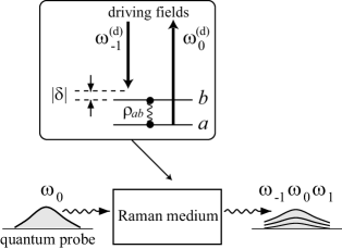
Figure 1: Principle of the technique: Two classical laser fields drive a Raman transition of molecules in a far-off-resonance medium. The beating of a weak quantum probe field with the prepared Raman coherence produces two new sideband fields.

We consider a far-off-resonance Raman medium, see Fig. 1. We send a pair of long, strong, classical laser fields, with carrier frequencies $\omega_{-1}^{(d)}$ and $\omega_{0}^{(d)}$, and a short, weak, quantum probe field $\hat{E}_{0}$, with carrier frequency $\omega_{0}$, through the Raman medium, along the $z$ direction. The timing and alignment of these fields are such that they substantially overlap with each other during the interaction process. The driving laser fields are tuned close to the Raman transition $|a\rangle\rightarrow|b\rangle$, with a small finite two-photon detuning $\delta$, but are far detuned from the upper electronic states of the molecules. These driving fields adiabatically produce a Raman coherence $\rho_{ab}$ some theory . When the probe field propagates through the medium, it beats with the Raman coherence prepared by the driving fields. Since the probe field is weak, the medium state does not change substantially during this step. The beating of the probe field with the prepared Raman coherence results in two new quantum fields $\hat{E}_{-1}$ and $\hat{E}_{1}$, at the Stokes and anti-Stokes frequencies $\omega_{-1}$ and $\omega_{1}$, respectively. We assume that the prepared Raman coherence $\rho_{ab}$ is substantial so that the spontaneous Raman processes are negligible compared to the stimulated processes. We also assume that the product of the coherence $\rho_{ab}$ and the medium length $L$ is not too large so that the generation of high-order sidebands of the probe field can be neglected. When we take the classical propagation equations for the Raman sidebands some theory and replace the field amplitudes by the quantum operators, we obtain

$$\frac{\partial\hat{E}_{0}}{\partial z}+\frac{\partial\hat{E}_{0}}{c\partial t} = i\beta_{0}(a_{0}\hat{E}_{0}+d_{-1}\rho_{ba}\hat{E}_{-1}+d_{0}\rho_{ab}\hat{E}_{1}),$$

$$\frac{\partial\hat{E}_{1}}{\partial z}+\frac{\partial\hat{E}_{1}}{c\partial t} = i\beta_{1}(a_{1}\hat{E}_{1}+d_{0}\rho_{ba}\hat{E}_{0}),$$

$$\frac{\partial\hat{E}_{-1}}{\partial z}+\frac{\partial\hat{E}_{-1}}{c\partial t} = i\beta_{-1}(a_{-1}\hat{E}_{-1}+d_{-1}\rho_{ab}\hat{E}_{0}).$$ (1)

Here, $a_{q}$ and $d_{q}$ with $q=0,\pm 1$ are the dispersion and coupling constants, respectively. We have denoted $\beta_{q}={\cal N}\hbar\omega_{q}/\epsilon_{0}c$, where ${\cal N}$ is the molecular number density.

We introduce the propagation constants $\kappa_{q}=\beta_{q}a_{q}$, and define the phase mismatch $\Delta k=2\kappa_{0}-\kappa_{1}-\kappa_{-1}$. We write $\rho_{ab}=\rho_{0}\exp[-i(\kappa_{1}-\kappa_{-1})z/2+i\phi_{0}]$, where $\rho_{0}\equiv|\rho_{ab}|$, and assume that $\rho_{0}$ and $\phi_{0}$ are constant in time and space. We change the variables by $\hat{E}_{0}=\hat{\cal E}_{0}\exp[i(\kappa_{0}-\Delta k/4)z]$ and $\hat{E}_{\pm 1}=\hat{\cal E}_{\pm 1}\exp[i(\kappa_{\pm 1}+\Delta k/4)z\mp i\phi_{0}]$. In terms of photon operators, we write $\hat{\cal E}_{q}(z,t)=(2\hbar\omega_{q}/\epsilon_{0}LA)^{1/2}\sum_{K}\hat{b}_{q}(K,t)e^{iK(z-ct)}$. Here, $L$ is the quantization length, which is taken to be equal to the medium length, $A$ is the quantization transverse area, which is taken to be equal to the beam area, $K$ is a Bloch wave vector, and $\hat{b}_{q}$ and $\hat{b}_{q}^{\dagger}$ are annihilation and creation operators for the $q$th mode. Then, we obtain

$$\frac{\partial\hat{b}_{0}}{\partial t} = i\Delta\hat{b}_{0}+i(g_{-1}\hat{b}_{-1}+g_{1}\hat{b}_{1}),$$

$$\frac{\partial\hat{b}_{\pm 1}}{\partial t} = -i\Delta\hat{b}_{\pm 1}+ig_{\pm 1}\hat{b}_{0},$$ (2)

where $\Delta={c\Delta k}/{4}$, $g_{1}=({\cal N}\hbar/\epsilon_{0})\sqrt{\omega_{1}\omega_{0}}\,d_{0}\rho_{0}$, and $g_{-1}=({\cal N}\hbar/\epsilon_{0})\sqrt{\omega_{-1}\omega_{0}}\,d_{-1}\rho_{0}$. It follows from Eqs. (2) that the boson operator commutation relations $[\hat{b}_{q},\hat{b}_{q^{\prime}}^{\dagger}]=\delta_{q,q^{\prime}}$ and $[\hat{b}_{q},\hat{b}_{q^{\prime}}]=[\hat{b}_{q}^{\dagger},\hat{b}_{q^{\prime}}^{\dagger}]=0$ are conserved in time. We also find that $\hat{b}_{0}^{\dagger}\hat{b}_{0}+\hat{b}_{1}^{\dagger}\hat{b}_{1}+\hat{b}_{-1}^{\dagger}\hat{b}_{-1}=\textrm{const}$, that is, the total photon number is conserved. Note that Eqs. (2) are the Heisenberg equations for the fields that are coupled to each other by the effective interaction Hamiltonian

$$\hat{H} = \hbar\Delta(\hat{b}_{1}^{\dagger}\hat{b}_{1}+\hat{b}_{-1}^{\dagger}\hat{b}_{-1}-\hat{b}_{0}^{\dagger}\hat{b}_{0})$$ (3)

$$\mbox{}-\hbar[g_{1}(\hat{b}_{0}\hat{b}_{1}^{\dagger}+\hat{b}_{1}\hat{b}_{0}^{\dagger})+g_{-1}(\hat{b}_{0}\hat{b}_{-1}^{\dagger}+\hat{b}_{-1}\hat{b}_{0}^{\dagger})].\quad$$

For simplicity, we restrict our discussion to the case where only a single mode of the probe field (with, e.g., $K=0$) is initially excited. Solving Eqs. (2), we find

$$\hat{b}_{q}(t)=\sum_{q^{\prime}}u_{qq^{\prime}}(t)\hat{b}_{q^{\prime}}(0),$$ (4)

where

$$u_{0,0}(t) = \cos(gt)+i(\Delta/g)\sin(gt),$$

$$u_{1,1}(t) = (g_{1}/g_{c})^{2}u_{0,0}^{*}(t)+(g_{-1}/g_{c})^{2}e^{-i\Delta t},$$

$$u_{-1,-1}(t) = (g_{-1}/g_{c})^{2}u_{0,0}^{*}(t)+(g_{1}/g_{c})^{2}e^{-i\Delta t},$$

$$u_{-1,1}(t) = u_{1,-1}(t)=(g_{1}g_{-1}/g_{c}^{2})\left[u_{0,0}^{*}(t)-e^{-i\Delta t}\right],$$

$$u_{0,\pm 1}(t) = u_{\pm 1,0}(t)=i(g_{\pm 1}/g)\sin(gt).$$ (5)

Here, we have denoted $g_{c}=\sqrt{g_{1}^{2}+g_{-1}^{2}}$ and $g=\sqrt{g_{c}^{2}+\Delta^{2}}$. When we introduce the boson operators $\hat{b}_{c}=(g_{1}\hat{b}_{1}+g_{-1}\hat{b}_{-1})/g_{c}$ and $\hat{b}_{u}=(g_{-1}\hat{b}_{1}-g_{1}\hat{b}_{-1})/g_{c}$, we can rewrite the solution (4) as

$$\hat{b}_{0}(t)=\cos(gt)\hat{b}_{0}(0)+i\sin(gt)[(\Delta/g)\hat{b}_{0}(0)+(g_{c}/g)\hat{b}_{c}(0)]$$ (6)

and

$$\hat{b}_{\pm 1}(t) = \pm(g_{\mp 1}/g_{c})e^{-i\Delta t}\hat{b}_{u}(0)+(g_{\pm 1}/g_{c})\cos(gt)\hat{b}_{c}(0)$$ (7)

$$\mbox{}+i\frac{g_{\pm 1}}{g}\sin(gt)[\hat{b}_{0}(0)-(\Delta/g_{c})\hat{b}_{c}(0)].$$

The boson operators $\hat{b}_{c}$ and $\hat{b}_{u}$ describe two orthogonal modes that are mixtures of the sideband fields. In terms of these operators, the effective Hamiltonian (3) has the form $\hat{H}=\hbar\Delta(\hat{b}_{u}^{\dagger}\hat{b}_{u}+\hat{b}_{c}^{\dagger}\hat{b}_{c}-\hat{b}_{0}^{\dagger}\hat{b}_{0})-\hbar g_{c}(\hat{b}_{0}\hat{b}_{c}^{\dagger}+\hat{b}_{c}\hat{b}_{0}^{\dagger})$. Unlike $\hat{b}_{c}$ and $\hat{b}_{c}^{\dagger}$, the operators $\hat{b}_{u}$ and $\hat{b}_{u}^{\dagger}$ are not coupled to the probe field operators $\hat{b}_{0}$ and $\hat{b}_{0}^{\dagger}$. Therefore, the modes described by $\hat{b}_{c}$ and $\hat{b}_{u}$ are called coupled and uncoupled modes, respectively. The uncoupled mode evolves in time as a harmonic oscillator with the frequency $\Delta$, that is, $\hat{b}_{u}(t)=\hat{b}_{u}(0)e^{-i\Delta t}$. Meanwhile, the coupled mode evolves in time as $\hat{b}_{c}(t)=\cos(gt)\hat{b}_{c}(0)+i\sin(gt)[(g_{c}/g)\hat{b}_{0}(0)-(\Delta/g)\hat{b}_{c}(0)]$. In terms of the coupled and uncoupled mode operators $\hat{b}_{c}$ and $\hat{b}_{u}$, the expressions of the sideband operators $\hat{b}_{1}$ and $\hat{b}_{-1}$ are given by $\hat{b}_{1}=(g_{1}\hat{b}_{c}+g_{-1}\hat{b}_{u})/g_{c}$ and $\hat{b}_{-1}=(g_{-1}\hat{b}_{c}-g_{1}\hat{b}_{u})/g_{c}$. In addition to the uncoupled mode described by $\hat{b}_{u}$, there are two other normal modes described by $\hat{b}_{+}=(\sqrt{g_{-}}\,\hat{b}_{0}-\sqrt{g_{+}}\,\hat{b}_{c})/\sqrt{2g}$ and $\hat{b}_{-}=(\sqrt{g_{+}}\,\hat{b}_{0}+\sqrt{g_{-}}\,\hat{b}_{c})/\sqrt{2g}$, where $g_{\pm}=g\pm\Delta$. They evolve in time as $\hat{b}_{+}(t)=\hat{b}_{+}(0)e^{-igt}$ and $\hat{b}_{-}(t)=\hat{b}_{-}(0)e^{igt}$, with the frequencies $g$ and $-g$, respectively. The inverse transformation yields $\hat{b}_{0}=(\sqrt{g_{-}}\,\hat{b}_{+}+\sqrt{g_{+}}\,\hat{b}_{-})/\sqrt{2g}$ and $\hat{b}_{c}=(\sqrt{g_{-}}\,\hat{b}_{-}-\sqrt{g_{+}}\,\hat{b}_{+})/\sqrt{2g}$. In terms of the normal mode operators, the effective Hamiltonian (3) has the diagonal form $\hat{H}=\hbar\Delta\hat{b}_{u}^{\dagger}\hat{b}_{u}+\hbar g(\hat{b}_{+}^{\dagger}\hat{b}_{+}-\hat{b}_{-}^{\dagger}\hat{b}_{-})$.

We note that the interaction between the probe field and the coupled mode field via the prepared Raman coherence is analogous to the interaction between the transmitted and reflected fields from a beam splitter Mandel and Scully book . However, the two mechanisms are very different in physical nature. The most important difference between them is that the two fields from the beam splitter have the same frequency while the coupled mode in the pump-probe Raman scheme is a superposition of the two sidebands with different Stokes and anti-Stokes frequencies.

For a Raman medium of the length $L$, the evolution time is $t=L/c$. The condition that $gL/c$ is small compared to unity is required for the negligibility of the generation of second- and higher-order sidebands some theory . In what follows we use the explicit expressions of the output operators $\hat{b}_{0,\pm 1}(L/c)$ to calculate various quantum statistical characteristics of the fields. We mostly restrict our discussion to the case where the Stokes and anti-Stokes sideband fields are initially in the vacuum state.

First, we calculate the correlation functions of the fields. We assume that the probe field is initially in an arbitrary state while the two sideband fields are initially in the vacuum state. Using Eqs. (6) and (7), we can easily calculate the normally ordered photon-number moments

$$\langle\hat{b}_{0}^{\dagger n}\hat{b}_{0}^{n}\rangle = \left[1-(g_{c}/g)^{2}\sin^{2}(gL/c)\right]^{n}\langle\hat{b}_{0}^{\dagger n}(0)\hat{b}_{0}^{n}(0)\rangle,$$

$$\langle\hat{b}_{\pm 1}^{\dagger n}\hat{b}_{\pm 1}^{n}\rangle = (g_{\pm 1}/g)^{2n}\sin^{2n}(gL/c)\langle\hat{b}_{0}^{\dagger n}(0)\hat{b}_{0}^{n}(0)\rangle.$$ (8)

Hence, the normalized $n$th-order autocorrelation functions $g_{q}^{(n)}=\langle\hat{b}_{q}^{\dagger n}\hat{b}_{q}^{n}\rangle/\langle\hat{b}_{q}^{\dagger}\hat{b}_{q}\rangle^{n}$ are found to be

$$g_{1}^{(n)}=g_{-1}^{(n)}=g_{0}^{(n)}=\frac{\langle\hat{b}_{0}^{\dagger n}(0)\hat{b}_{0}^{n}(0)\rangle}{\langle\hat{b}_{0}^{\dagger}(0)\hat{b}_{0}(0)\rangle^{n}}.$$ (9)

In particular, the normalized second-order autocorrelation functions are obtained as $g_{1}^{(2)}=g_{-1}^{(2)}=g_{0}^{(2)}=\langle\hat{n}_{0}^{\textrm{(in)}}(\hat{n}_{0}^{\textrm{(in)}}-1)\rangle/\langle\hat{n}_{0}^{\textrm{(in)}}\rangle^{2}$. Here, $\hat{n}_{0}^{\textrm{(in)}}\equiv\hat{b}_{0}^{\dagger}(0)\hat{b}_{0}(0)$ is the photon-number operator for the probe field at the input. Thus, the generated sideband fields and the probe field have the same normalized autocorrelation functions, which are independent of the evolution time and are solely determined by the statistical properties of the input probe field. In other words, the normalized autocorrelation functions of the probe field do not change during the beating process and are precisely replicated to the generated sideband fields. In particular, if the photon statistics of the input probe field is sub-Poissonian, Poissonian, or super-Poissonian, the photon statistics of the sideband fields will also be sub-Poissonian, Poissonian, or super-Poissonian, respectively. Such a replication of the normalized autocorrelation characteristics is called autocorrelation multiplexing. This result is in agreement with the conclusions of the experiments on replication of multimode laser radiation Liang and broadband incoherent light Katsuragawa . The ability of the Raman medium to multiplex the autocorrelation characteristics is similar to but, because of the change in carrier frequency, somewhat different from the property of a beam splitter Mandel and Scully book .

The normalized two-mode cross-correlation functions are defined by $g_{kl}^{(2)}=\langle\hat{n}_{k}\hat{n}_{l}\rangle/(\langle\hat{n}_{k}\rangle\langle\hat{n}_{l}\rangle)$, where $k\not=l$ and $\hat{n}_{q}=\hat{b}_{q}^{\dagger}\hat{b}_{q}$. Using Eqs. (6) and (7), we find

$$g_{0,1}^{(2)}=g_{0,-1}^{(2)}=g_{1,-1}^{(2)}=\frac{\langle\hat{n}_{0}^{\textrm{(in)}}(\hat{n}_{0}^{\textrm{(in)}}-1)\rangle}{\langle\hat{n}_{0}^{\textrm{(in)}}\rangle^{2}}.$$ (10)

Thus, the normalized two-mode cross-correlation functions are equal to each other and to the normalized second-order autocorrelation functions of the fields. Note that the correlations between the modes are nonzero, that is, $g_{kl}^{(2)}\not=1$ ($k\not=l$), only if the photon statistics of the input probe field is not Poissonian. With respect to these properties, the Raman scheme is also similar to a beam splitter Mandel and Scully book except for the fact that the modes in the Raman medium have different frequencies.

Second, we examine the squeezing of the field quadratures in the case where the two sideband fields are initially in the vacuum state. A field quadrature of the $q$th mode is defined by $\hat{X}_{q}=\hat{b}_{q}^{\dagger}e^{i\varphi}+\hat{b}_{q}e^{-i\varphi}$. We say that the $q$th mode is in a squeezed state if there exists such a phase $\varphi$ that $\langle(\Delta\hat{X}_{q})^{2}\rangle<1$ or, equivalently, $S_{q}<0$, where $S_{q}=\langle(\Delta\hat{X}_{q})^{2}\rangle-1=2[\langle\hat{b}_{q}^{\dagger}\hat{b}_{q}\rangle-\langle\hat{b}_{q}^{\dagger}\rangle\langle\hat{b}_{q}\rangle]+[(\langle\hat{b}_{q}^{2}\rangle-\langle\hat{b}_{q}\rangle^{2})e^{-2i\varphi}+\textrm{c.c.}]$. The squeezing degree is measured by the quantity $-S_{q}$. Using Eqs. (6) and (7), we find

$$S_{0}(\varphi) = [1-(g_{c}/g)^{2}\sin^{2}(gL/c)]S_{0}^{\textrm{(in)}}(\varphi-\varphi_{L}),$$

$$S_{\pm 1}(\varphi) = (g_{\pm 1}/g)^{2}\sin^{2}(gL/c)S_{0}^{\textrm{(in)}}(\varphi-\pi/2).$$ (11)

Here, $\varphi_{L}=\arctan[(\Delta/g)\tan(gL/c)]$ is an angle, and $S_{0}^{\textrm{(in)}}(\varphi)$ is the squeezing factor for the $\varphi$-quadrature of the input probe field. We find from Eqs. (11) that, if $S_{0}^{\textrm{(in)}}(\varphi)<0$, then $S_{\pm 1}(\varphi+\pi/2)<0$. Thus, if the input probe field is in a squeezed state, then the generated sideband fields are also in squeezed states. In other words, the squeezing of the input probe field is transfered to the sideband fields during the beating process. The squeezing factors $S_{\pm 1}(\varphi+\pi/2)$ of the sideband fields are reduced from the squeezing factor $S_{0}(\varphi)$ of the input probe field by the factors $(g_{\pm 1}/g)^{2}\sin^{2}(gL/c)$, and the phases of the squeezed quadratures change by $\pi/2$. This result can be used to convert (partially) squeezing to a new frequency, i.e., to perform partial squeezing multiplexing. We note that the normalized squeezing factors $s_{q}\equiv S_{q}/\langle\hat{n}_{q}\rangle$ satisfy the relations $s_{1}(\varphi+\pi/2)=s_{-1}(\varphi+\pi/2)=s_{0}(\varphi+\varphi_{L})=s_{0}^{\textrm{(in)}}(\varphi)$. Consequently, these normalized factors have the same maximal and minimal values for all the three fields. We also note that, when the input probe field is in a coherent state, the sideband fields have no squeezing. This property is similar to the case of four-wave mixing but is unlike the case of degenerate parametric down-conversion, where perfect squeezing can in principle be obtained.

Next, we calculate the state of the fields in a special case where the input probe field is in a coherent state $|\alpha\rangle_{0}$ and the two sideband fields are initially in the vacuum state. The state of the fields at the input is

$$|\Psi_{\textrm{in}}\rangle=|0\rangle_{-1}|\alpha\rangle_{0}|0\rangle_{1}=e^{-|\alpha|^{2}/2}e^{\alpha\hat{b}_{0}^{\dagger}(0)}|0\rangle.$$ (12)

The state of the fields at the output is given by $|\Psi_{\textrm{out}}\rangle=\hat{U}(L/c)|\Psi_{\textrm{in}}\rangle$, where $\hat{U}(L/c)=\exp(-i\hat{H}L/\hbar c)$. Since $\hat{U}(L/c)|0\rangle=|0\rangle$, we have $|\Psi_{\textrm{out}}\rangle=e^{-|\alpha|^{2}/2}e^{\alpha\hat{b}_{0}^{\dagger}(-L/c)}|0\rangle$. Using Eq. (6), we find

$$|\Psi_{\textrm{out}}\rangle=|\alpha_{-1}(L/c)\rangle_{-1}|\alpha_{0}(L/c)\rangle_{0}|\alpha_{1}(L/c)\rangle_{1}.$$ (13)

Here, $|\alpha_{q}(L/c)\rangle_{q}$ is a coherent state of the $q$th mode, with the amplitude $\alpha_{q}(L/c)=\alpha u_{0q}(L/c)$. Thus, a probe field in a coherent state can produce two sideband fields that are also in coherent states. Such a process is called coherent-state multiplexing. This property of the Raman medium is also similar to that of a beam splitter Mandel and Scully book except for the fact that there is a change of the carrier frequency in the Raman scattering process.

Finally, we calculate the state of the output field for the case where the input state of the probe field is a Fock state $|n\rangle_{0}$ and the input state of the sideband fields is the vacuum state. The state of the fields at the input is

$$|\Psi_{\textrm{in}}\rangle=|0\rangle_{-1}|n\rangle_{0}|0\rangle_{1}=\frac{\hat{b}_{0}^{\dagger n}(0)}{\sqrt{n!}}|0\rangle.$$ (14)

The state of the fields at the output is given by $|\Psi_{\textrm{out}}\rangle=[\hat{b}_{0}^{\dagger n}(-L/c)/\sqrt{n!}]|0\rangle$. With the help of Eq. (6), the state of the fields at the output is found to be

$$|\Psi_{\textrm{out}}\rangle = \sum_{l=0}^{n}\sum_{m=0}^{l}\left(\begin{array}[]{c}n\\ l\end{array}\right)^{1/2}\left(\begin{array}[]{c}l\\ m\end{array}\right)^{1/2}$$ (20)

$$\mbox{}\times u_{0,-1}^{l-m}(L/c)u_{0,0}^{n-l}(L/c)u_{0,1}^{m}(L/c)$$

$$\mbox{}\times|l-m\rangle_{-1}|n-l\rangle_{0}|m\rangle_{1}.$$

In general, expression (20) stands for a tripartite entangled state. Tripartite entangled states can find various applications in quantum information Zeilinger ; Chuan .

More generally, we can show that an arbitrary coherent state $|\alpha_{-1}(0),\alpha_{0}(0),\alpha_{1}(0)\rangle$ of the input fields produces a coherent state $|\alpha_{-1}(L/c),\alpha_{0}(L/c),\alpha_{1}(L/c)\rangle$ of the output fields, where $\alpha_{q}(L/c)=\sum_{q^{\prime}}u_{qq^{\prime}}(L/c)\alpha_{q^{\prime}}(0)$. Consequently, the diagonal coherent-state representation $P_{\textrm{in}}(\{\alpha_{q}\})$ of an arbitrary state $\hat{\rho}_{\textrm{in}}$ of the input fields determines the representation $P_{\textrm{out}}(\{\alpha_{q}\})$ of the state $\hat{\rho}_{\textrm{out}}$ the output fields via the equation

$$P_{\textrm{out}}(\{\alpha_{q}\})=P_{\textrm{in}}(\{\sum_{q^{\prime}}u_{qq^{\prime}}^{*}(L/c)\alpha_{q^{\prime}}\}).$$ (21)

If the input state $\hat{\rho}_{\textrm{in}}$ is a classical state Mandel and Scully book , $P_{\textrm{in}}(\{\alpha_{q}\})$ must be non-negative and less singular than a delta function, and consequently so must $P_{\textrm{out}}(\{\alpha_{q}\})$. In this case, the output state $\hat{\rho}_{\textrm{out}}$ is also a classical state. Moreover, since the coherent state $|\alpha_{-1},\alpha_{0},\alpha_{-1}\rangle$ is separable and the weight factor $P_{\textrm{out}}(\{\alpha_{q}\})$ is non-negative, the output state $\hat{\rho}_{\textrm{out}}$ is, by definition, separable Chuan ; Zeilinger . Therefore, a necessary condition for the output fields to be in an entangled state or, more generally, in a nonclassical state is that the input field state is a nonclassical state. A similar condition has been derived for the beam splitter entangler Knight . Note that, in the case where the two sideband fields are initially in the vacuum state, Eq. (21) reduces to $P_{\textrm{out}}(\{\alpha_{q}\})=P_{\textrm{in}}^{(0)}(\sum_{q}u_{0q}^{*}\alpha_{q})\delta(\sum_{q}u_{1q}^{*}\alpha_{q})\delta(\sum_{q}u_{-1q}^{*}\alpha_{q})$, where $P_{\textrm{in}}^{(0)}(\alpha)$ is the coherent-state representation of an arbitrary state of the input probe field.

In conclusions, we have shown that the parametric beating of a quantum probe field with a prepared Raman coherence can replicate the normalized autocorrelation functions into the Stokes and anti-Stokes sidebands. We have found that an initial coherent state of the probe field can be replicated to the Raman sidebands, and an initial squeezing of the probe field can be partially transferred to the sidebands. We have shown that a necessary condition for the fields at the output of the Raman medium to be in an entangled state or, more generally, in a nonclassical state is that the input field state is a nonclassical state. We emphasize that, for the validity of our model, the prepared Raman coherence should be substantial (so that the effect of the probe on the coherence is negligible), but the product of the coherence and the medium length should not be too large (because otherwise high-order sidebands would be involved). Such Raman excitation level can be produced by applying the two-color adiabatic Raman pumping technique for far-off-resonance Raman media, such as solid hydrogen, molecular hydrogen gas, and deuterium gas Liang ; Katsuragawa ; Modulation ; some theory . The pump-probe Raman scheme is characterized by high conversion efficiency and therefore can provide a good tool to replicate quantum statistical characteristics from one mode to another.

Useful discussions with S. Dutta-Gupta and A. K. Patnaik are gratefully acknowledged.

References

• (1) A. Nazarkin, G. Korn, M. Wittmann, and T. Elsaesser, Phys. Rev. Lett. 83, 2560 (1999).
• (2) V. P. Kalosha and J. Herrmann, Phys. Rev. Lett. 85, 1226 (2000); V. P. Kalosha and J. Herrmann, Opt. Lett. 26, 456 (2001); Fam Le Kien, Nguyen Hong Shon, and K. Hakuta, Phys. Rev. A 64, 051803(R) (2001); Fam Le Kien, K. Hakuta, and A. V. Sokolov, Phys. Rev. A 66, 023813 (2002); V. Kalosha, M. Spanner, J. Herrmann, and M. Ivanov, Phys. Rev. Lett. 88, 103901 (2002); R. A. Bartels, T. C. Weinacht, N. Wagner, M. Baertschy, Chris H. Greene, M. M. Murnane, and H. C. Kapteyn, Phys. Rev. Lett. 88, 013903 (2002);
• (3) J. Q. Liang, M. Katsuragawa, Fam Le Kien, and K. Hakuta, Phys. Rev. Lett. 85, 2474 (2000).
• (4) M. Katsuragawa, J. Q. Liang, Fam Le Kien, and K. Hakuta, Phys. Rev. A 65, 025801 (2002).
• (5) S. E. Harris and A. V. Sokolov, Phys. Rev. A 55, R4019 (1997); A. V. Sokolov, D. D. Yavuz, S. E. Harris, Opt. Lett. 24, 557 (1999); A. V. Sokolov, D. R. Walker, D. D. Yavuz, G. Y. Yin, and S. E. Harris, Phys. Rev. Lett. 85, 562 (2000); A. V. Sokolov, D. D. Yavuz, D. R. Walker, G. Y. Yin, and S. E. Harris, Phys. Rev. A 63, 051801(R) (2001).
• (6) S. E. Harris and A. V. Sokolov, Phys. Rev. Lett. 81, 2894 (1998); Fam Le Kien, J. Q. Liang, M. Katsuragawa, K. Ohtsuki, K. Hakuta, and A. V. Sokolov, Phys. Rev. A 60, 1562 (1999).
• (7) A. V. Sokolov, D. R. Walker, D. D. Yavuz, G. Y. Yin, and S. E. Harris, Phys. Rev. Lett. 87, 033402 (2001).
• (8) N. Zhavoronkov and G. Korn, Phys. Rev. Lett. 88, 203901 (2002).
• (9) S. E. Harris, D. R. Walker, and D. D. Yavuz, Phys. Rev. A 65, 021801(R) (2002).
• (10) A. S. Zibrov, A. B. Matsko, O. Kocharovskaya, Y. V. Rostovtsev, G. R. Welch, and M. O. Scully, Phys. Rev. Lett. 88, 103601 (2002).
• (11) See, for example, L. Mandel and E. Wolf, Optical Coherence and Quantum Optics (Cambridge University Press, New York, 1995) and M. Scully and S. Zubairy, Quantum Optics (Cambridge University Press, New York, 1997).
• (12) See also L. J. Wang, C. K. Hong, and S. R. Friberg, J. Opt. B: Quantum Semiclass. Opt. 3, 346 (2001) and references therein.
• (13) The Physics of Quantum Information, edited by D. Bouwmeester, A. K. Ekert, and A. Zeilinger (Springer, New York, 2000).
• (14) M. A. Nielsen and I. L. Chuan, Quantum Computation and Quantum Information (Cambridge University Press, New York, 2000).
• (15) M. S. Kim, W. Son, V. BuΕΎek, and P. L. Knight, Phys. Rev. A 65, 032323 (2002); Wang Xiang-bin, ibid. 66, 024303 (2002).