Investigating three qubit entanglement with local
measurements

Abstract: In this paper we describe how three qubit entanglement can be analyzed with local measurements. For this purpose we decompose entanglement witnesses into operators which can be measured locally. Our decompositions are optimized in the number of measurement settings needed for the measurement of one witness. Our method allows to detect true threepartite entanglement and especially GHZ-states with only four measurement settings.

1 Introduction

Entanglement is one of the most puzzling features of quantum theory and of great importance for quantum information theory. It is the resource that makes various quantum protocols possible that perform certain tasks better than it would be possible with purely classical methods [1]. The investigation and characterization of entanglement with experimental and theoretical methods itself is therefore a task of great importance.

From an experimental point of view it is important to find effective techniques for the production and detection of entanglement. For the detection of entanglement several strategies are known: One can determine the whole density matrix [2] and then try to apply one of the necessary or sufficient entanglement criteria, e.g. the PPT criterion [3, 4]. One can also look for a violation of Bell inequalities [5]. Furthermore, there have been several proposals of detecting entanglement without estimating the whole density matrix [6, 7].

However, all these nice ideas have also some disadvantages. Estimating the whole density matrix requires a lot of measurements, and in fact one does not need to know the whole matrix in order to check whether it is entangled or not. On the other hand, looking for a violation of Bell inequalities may not suffice for a making a decision, since there are entangled states which do not violate any known Bell inequality [8, 9, 10]. It has even been conjectured that entangled states with a positive partial transpose do not violate any Bell inequality at all [11]. Finally, the recent proposals of detection require collective measurements on several qubits which makes them hard to implement with the present techniques.

Furthermore, the schemes mentioned above are in some sense too general for many experimental situations. They assume that no a priori information about the state is given. However, in a typical experimental situation one often tries to prepare a certain pure state. Due to imperfections of the experimental apparatus the output state will be a mixture of the desired state and some noise instead. In this case it is desirable to know whether the produced state is still entangled or not.

In [12, 13] we proposed a general scheme for entanglement detection for the case that some knowledge about the state is given. In this scheme we only want to use local projective measurements, since these measurements can easily be implemented in a lab. In addition, we would like to decrease the number of measurements needed to the minimum, of course.

The scheme relies on the well known concept of witness operators [4, 14]. An hermitean operator $W$ is called a witness operator (or entanglement witness) detecting the entangled state $\varrho_{e}$ if $Tr(W\varrho_{e})<0$ while $Tr(W\varrho_{s})\geq 0$ holds for all separable states $\varrho_{s}.$ Thus if a measurement yields $Tr(W\varrho)<0$ then the state $\varrho$ is entangled with certainty. As a consequence of the Hahn-Banach theorem it follows that for every entangled state $\varrho_{e}$ there exists such an entanglement witness and for many states it is known how to construct such witnesses [15]. After having constructed the witness, we decompose it into a sum of local measurements, then the expectation value can be measured with simple methods. This decomposition has to be optimized in a certain way since we want to use the smallest number of measurements possible.

Our paper is organized as follows: The first section deals with the decomposition into local measurements because this is the core of our approach. We define there what we understand by an optimized decomposition. We would like to remark here that finding optimized decompositions is in general a hard task, much harder than constructing entanglement witnesses. In the second section we illustrate our approach with an example of a two qubit system. We construct the witness and determine its optimal decomposition. Finally in the third and main part we apply this idea to three qubit systems. We explain how GHZ-type and W-type entanglement can be detected with local measurements. We also determine the minimal number of measurements needed for this.

2 Local decompositions

Assume that we have an hermitean operator $H$ acting on a tensor product $\mathcal{H}=\mathcal{H}_{A}\otimes\mathcal{H}_{B}\otimes...\otimes\mathcal{H}_{Z}$ of two or more (but finite) dimensional Hilbert spaces. In order to slenderize the notation we look here at the case that we have a bipartite $N\times N$-system: $\mathcal{H}=\mathcal{H}_{A}\otimes\mathcal{H}_{B}$ with $\mbox{dim}(\mathcal{H}_{A})=\mbox{dim}(\mathcal{H}_{B})=N.$ But all definitions in this section can be extended to more parties in an obvious manner. In order to measure the expectation value of this operator locally, we have to decompose it in a sum of tensor products of operators acting on only one system, or, equivalently, we have to decompose it into a sum of projectors onto product vectors:

$$H=\sum_{i=1}^{m}A_{i}\otimes B_{i}=\sum_{i=1}^{n}c_{i}|e_{i}\rangle\langle e_{i}|\otimes|f_{i}\rangle\langle f_{i}|.$$ (1)

By measuring the expectation value of the projectors $|e_{i}\rangle\langle e_{i}|\otimes|f_{i}\rangle\langle f_{i}|$ and adding the results with the weights $c_{i}$ this decomposition (1) can be measured locally. There are, of course, many possibilities of finding a decomposition like (1). So we have to optimize the decomposition in a certain sense. But there are even several possibilities of defining an optimized decomposition.

On the first sight one might try to minimize the number of product vectors corresponding to minimizing $n$ in (1). This optimization procedure is already known from the literature, it was considered in [16]. There it was shown that for a general operator acting on two qubits one needs five product vectors and also a constructive way of computing these product vectors was given.

However, since we want to construct an experimentally accessible scheme for entanglement detection it is natural to look for a decomposition where Alice and Bob have to perform the smallest number of measurements possible. By “measurements” we understand here von Neumann (or projective) measurements, since they can be easily implemented. Such a measurement for Alice corresponds to a choice of an orthonormal basis of $\mathcal{H}_{A},$ and Bob has to choose an orthonormal basis $\mathcal{H}_{B}$, too. So any operator of the form

$$M=\sum_{k,l=1}^{N}c_{kl}|e_{k}\rangle\langle e_{k}|\otimes|f_{l}\rangle\langle f_{l}|$$ (2)

with $\langle e_{s}|e_{t}\rangle=\langle f_{s}|f_{t}\rangle=\delta_{st}$ can be measured with only one collective setting of measurement devices of Alice and Bob. Alice and Bob can distinguish the states $|e_{k}f_{l}\rangle,$ measure the probabilities of these states and add their results with the weights $c_{kl}$ to measure $M.$ We call an operator which can be measured with one measurement setting (like $M$ in Eq. (2)) a local von Neumann measurement (LvNM).

Having understood what can be realized with one measurement setting, we can state another optimization strategy. We want to find a decomposition of the form

$$H=\sum_{i=1}^{k}\sum_{k,l=1}^{N}c^{i}_{kl}|e^{i}_{k}\rangle\langle e^{i}_{k}|\otimes|f^{i}_{l}\rangle\langle f^{i}_{l}|$$ (3)

with $\langle e^{i}_{s}|e^{i}_{t}\rangle=\langle f^{i}_{s}|f^{i}_{t}\rangle=\delta_{st}$ and a minimal $k.$ This $k$ is the number of collective measurement settings Alice and Bob have to use in order to measure $H.$ This optimization strategy is the aim we are considering in this paper when we talk about “optimized” decompositions.

The reader should note that minimizing $m$ in (1) is not the same as our optimization strategy. However, for systems of dimension $N$ greater than 2 it might be more suitable to decompose the witness as $W=\sum_{i}^{m}A_{i}\otimes B_{i}$. As shown in [17], the expectation values of operators $A_{i}$ or $B_{i}$ can be measured by a POVM with a single qubit as ancilla instead of counting clicks for all possible N outcomes of the operator. Also minimizing the number of product vectors (i.e. minimizing $n$ in (1)) is not the same. This will become clear in a few seconds, when we study two qubits.

3 Two qubits

We illustrate the method by considering an experiment that aims at producing a certain 2-qubit state $|\Psi\rangle=a|01\rangle+b|10\rangle$ written in the Schmidt decomposition, i.e. $a,b\geq 0,a^{2}+b^{2}=1.$ Due to imperfections, the produced state will rather be

$$\varrho_{p,d}=p|\Psi\rangle\langle\Psi|+(1-p)\sigma,$$ (4)

where we assume that the noise state $\sigma$ lies inside a separable ball of radius $d$ around the totally mixed state, i.e. $\|\sigma-\mathbbm{1}/4\|\leq d$ for some norm. Our aim is to provide a local experimental method to tell whether the produced state is entangled or not, based on witness operators.

Since we only want to explain our basic idea, we assume here that we have white noise, this means $d=0.$ The case $d>0$ is studied in greater detail in [13]. We would like to stress that our assumption $d=0$ is in some sense artificial. By this we mean that if $d=0$ there is a simple way of determining whether $\varrho_{p,0}$ is entangled or not: One can just measure any operator $A$ (which fulfills $Tr(A)\neq 4Tr(A|\psi\rangle\langle\psi|)$) and compute $p$ from the expectation value of this operator. With this information the density matrix $\varrho_{p,0}$ can be constructed and the PPT criterion can be used to decide whether it is entangled or not. This is not possible for obvious reasons if $d>0$.

To reach our goal we first have to construct a proper entanglement witness. For NPPT entangled states, i.e. entangled states with a non-positive partial transpose, the construction of a witness is relatively easy: The partial transpose of a projector onto an eigenvector of $\varrho^{T_{B}}$ with negative eigenvalue does the job. Here $T_{B}$ denotes the partial transposition with respect to subsystem $B.$

The state $\varrho_{p,0}$ has one possibly negative eigenvalue, namely ${\lambda_{-}}=(1-p)/4-abp$, with the corresponding eigenvector

$$|\psi_{-}\rangle=\frac{1}{\sqrt{2}}(|00\rangle-|11\rangle)$$ (5)

that is independent of $a$ and $p$. Then $W_{0}=|\psi_{-}\rangle\langle\psi_{-}|^{T_{B}}$ is an entanglement witness detecting $\varrho_{p,0}$ since

$$Tr(|\psi_{-}\rangle\langle\psi_{-}|^{T_{B}})\varrho_{p,0}=Tr|\psi_{-}\rangle\langle\psi_{-}|(\varrho_{p,0}^{T_{B}})={\lambda_{-}}<0.$$ (6)

Having constructed the witness, all that remains is to decompose it. Defining $|z^{\pm}\rangle=|0,1\rangle$, $|x^{\pm}\rangle=(|0\rangle\pm|1\rangle)/\sqrt{2}$ and $|y^{\pm}\rangle=(|0\rangle\pm i|1\rangle)/\sqrt{2}$ we can decompose the more general witness $|\phi\rangle\langle\phi|^{T_{B}}$ for $|\phi\rangle=\alpha|00\rangle+\beta|11\rangle$ as follows:

$${|\phi\rangle\langle\phi|^{T_{B}}} = \alpha^{2}|00\rangle\langle 00|+\beta^{2}|11\rangle\langle 11|+\alpha\beta(|01\rangle\langle 10|+|10\rangle\langle 01|)$$ (7)

$$= \alpha^{2}|z^{+}z^{+}\rangle\langle z^{+}z^{+}|+\beta^{2}|z^{-}z^{-}\rangle\langle z^{-}z^{-}|+\alpha\beta\left(|x^{+}x^{+}\rangle\langle x^{+}x^{+}|+\right.$$

$$\left.+|x^{-}x^{-}\rangle\langle x^{-}x^{-}|-|y^{+}y^{-}\rangle\langle y^{+}y^{-}|-|y^{-}y^{+}\rangle\langle y^{-}y^{+}|\right)$$

$$= \frac{1}{4}\left(\mathbbm{1}\otimes\mathbbm{1}+\sigma_{z}\otimes\sigma_{z}+(\alpha^{2}-\beta^{2})(\sigma_{z}\otimes\mathbbm{1}+\mathbbm{1}\otimes\sigma_{z})\right.$$

$$\left.+2\alpha\beta(\sigma_{x}\otimes\sigma_{x}+\sigma_{y}\otimes\sigma_{y})\right),$$

where the $\sigma_{i}$ are the Pauli matrices. This way of decomposing a witness can be used for higher dimensions and for systems of more than 2 parties by using

$$|01\rangle\langle 10|+|10\rangle\langle 01| = |x^{+}x^{+}\rangle\langle x^{+}x^{+}|+|x^{-}x^{-}\rangle\langle x^{-}x^{-}|-$$ (8)

$$-|y^{+}y^{-}\rangle\langle y^{+}y^{-}|-|y^{-}y^{+}\rangle\langle y^{-}y^{+}|.$$

The local measurement of the general witness of Eq. (7) requires three measurements of Alice and of Bob in the $x,y$ and $z$ direction. This is also true for the special case $\alpha=-\beta=1/\sqrt{2}$ corresponding to $W_{0}$. It is not possible to evaluate the witness with less than three LvNMs:

Proposition 1. The witness $W_{0}$ can not be decomposed into less than three LvNMs, therefore the decomposition (7) is optimal.
Proof. The proof was first given in [12], we repeat it here because we extend it later to three qubit systems. Consider a decomposition requiring two measurements:

$${|\psi\rangle\langle\psi|}^{T_{B}}=\sum_{i,j=0}^{1}c^{1}_{ij}|A^{1}_{i}\rangle\langle A^{1}_{i}|\otimes|B^{1}_{j}\rangle\langle B^{1}_{j}|+\sum_{i,j=0}^{1}c^{2}_{ij}|A^{2}_{i}\rangle\langle A^{2}_{i}|\otimes|B^{2}_{j}\rangle\langle B^{2}_{j}|,$$ (9)

where $\{|A_{i}\rangle\}$ and $\{|B_{i}\rangle\}$ are orthonormal bases for $\mathcal{H}_{A}$ and $\mathcal{H}_{B}$, respectively. With the help of a Schmidt decomposition as above we can write ${|\psi\rangle\langle\psi|}^{T_{B}}=\sum_{i,j=0}^{3}\lambda_{ij}\;\sigma_{i}\otimes\sigma_{j}$ with

$$(\lambda_{ij})=\left(\begin{array}[]{cccc}\frac{1}{4}&0&0&\frac{\alpha^{2}-\beta^{2}}{4}\\ 0&\frac{\alpha\beta}{2}&0&0\\ 0&0&\frac{\alpha\beta}{2}&0\\ \frac{\alpha^{2}-\beta^{2}}{4}&0&0&\frac{1}{4}\end{array}\right).$$ (10)

Note that the $3\times 3$ sub-matrix in the right bottom corner is of rank 3. Now we write any projector on the rhs of (9) as a vector in the Bloch sphere: $|A^{1}_{0}\rangle\langle A^{1}_{0}|=\sum_{i=0}^{3}s^{A}_{i}\sigma_{i}$ is represented by the vector $s^{A^{1}_{0}}=(1/2,s^{A}_{1},s^{A}_{2},s^{A}_{3})$ and $|A^{1}_{1}\rangle\langle A^{1}_{1}|$ by $s^{A^{1}_{1}}=(1/2,-s^{A}_{1},-s^{A}_{2},-s^{A}_{3});$ $|B^{1}_{0}\rangle\langle B^{1}_{0}|$ can be written similarly. If we expand the first sum on the rhs of (9) in the ($\sigma_{i}\otimes\sigma_{j}$) basis, the $3\times 3$ sub-matrix in the right bottom corner is given by $(c^{1}_{00}-c^{1}_{01}-c^{1}_{10}+c^{1}_{11})(s^{A}_{1},s^{A}_{2},s^{A}_{3})^{T}(s^{B}_{1},s^{B}_{2},s^{B}_{3}).$ This matrix is of rank one. The corresponding sub-matrix from the second LvNM on the rhs of (9) is also of rank one and we arrive at a contradiction: No matrix of rank three can be written as a sum of two matrices of rank one.$\hfill\Box$

Please note that the decomposition (7) requires 6 projectors onto product vectors (PPV). By applying the method of [16] it is possible to decompose the witness using only 5 PPV:

$$|\psi\rangle\langle\psi|^{T_{B}}=\frac{(\alpha+\beta)^{2}}{3}\sum_{i=1}^{3}|A^{\prime}_{i}A^{\prime}_{i}\rangle\langle A^{\prime}_{i}A^{\prime}_{i}|-\alpha\beta(|01\rangle\langle 01|+|10\rangle\langle 10|),$$ (11)

where we have used the definitions

$$|A^{\prime}_{1}\rangle = e^{i\frac{\pi}{3}}\cos(\theta)|0\rangle+e^{-i\frac{\pi}{3}}\sin(\theta)|1\rangle$$ (12)

$$|A^{\prime}_{2}\rangle = e^{-i\frac{\pi}{3}}\cos(\theta)|0\rangle+e^{i\frac{\pi}{3}}\sin(\theta)|1\rangle$$

$$|A^{\prime}_{3}\rangle = |A^{\prime}_{1}\rangle+|A^{\prime}_{2}\rangle$$

$$\cos(\theta) = \sqrt{\alpha/(\alpha+\beta)}$$

$$\sin(\theta) = \sqrt{\beta/(\alpha+\beta)}.$$ (13)

However, with this decomposition the measurement of the witness would require 4 local correlated measurement settings, hence the two optimization strategies are really different.

4 Three qubits

The state space for three qubits has a much richer structure concerning entanglement than the space of two qubits. Let us briefly remind the reader of some well known facts about three qubits. We first consider pure states. There are two classes of states which are not genuine threepartite entangled: The fully separable states, which can be written as

$$|\phi_{fs}\rangle_{ABC}=|\alpha\rangle_{A}\otimes|\beta\rangle_{B}\otimes|\gamma\rangle_{C},$$ (14)

and the biseparable states which can be written as a product state in the bipartite system, which is created, if two of the three qubits are grouped together to one party. One example is

$$|\phi_{bs}\rangle_{A-BC}=|\alpha\rangle_{A}\otimes|\delta\rangle_{BC}.$$ (15)

There are three possibilities of grouping two qubits together, hence there are three classes of biseparable states. The genuine threepartite entangled states are the states which are neither fully separable nor biseparable. Given two threepartite states, $|\phi\rangle$ and $|\psi\rangle,$ one can ask whether it is possible to transform $|\phi\rangle$ into $|\psi\rangle$ with local operations and classical communication, without requiring that this can be done with probability 1. These operations are called stochastic local operations and classical communication (SLOCC). It turns out [18] that $|\phi\rangle$ can be transformed into $|\psi\rangle$ iff there exist operators $A,B,C,$ acting on the space of one qubit with

$$|\psi\rangle=A\otimes B\otimes C|\phi\rangle.$$ (16)

Surprisingly, it was proven in [18] that there are two classes of genuine threepartite entangled states which cannot be transformed into another by SLOCC. One class, the class of GHZ-states can be transformed by SLOCC into

$$|GHZ\rangle=1/\sqrt{2}(|000\rangle+|111\rangle),$$ (17)

the other class, the class of W-states can be converted into

$$|W\rangle=1/\sqrt{3}(|100\rangle+|010\rangle+|001\rangle.$$ (18)

Now we can classify the mixed states according to [19]. We define a mixed state $\varrho$ as fully separable if $\varrho$ can be written as a convex combination of fully separable pure states. A state $\varrho$ which is not fully separable is called biseparable if it can be written as a convex combination of biseparable pure states. One can, of course, define three classes of biseparable mixed states with respect of one of the three partitions as well. Finally, $\varrho$ is fully entangled if it is neither biseparable nor fully separable. There are again two classes of fully entangled mixed states, the W-class and the GHZ-class. $\varrho$ belongs to the W-class, if it can be written as a convex combination of pure W- states, and to the GHZ-class otherwise. Taking into account that the set of all states is also a convex set, one obtains an “onion”-structure. This structure is shown in Fig. 1.

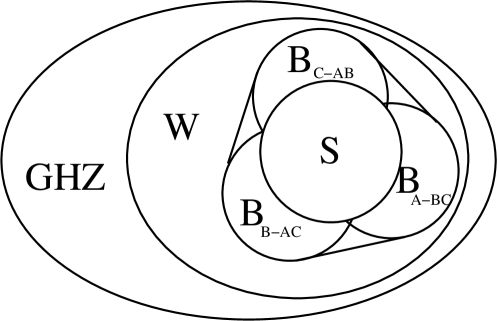
Figure 1: The structure of the set of three qubit states: They can be (S)eparable, (B)iseparable, (W)-entangled, or (GHZ)-entangled.

In the same reference also witnesses for the detection of GHZ-type and W-type states have been constructed. Here a want to compute the optimized decompositions of these operators.

For the GHZ-class a witness operator is given by

$$W_{GHZ}=\frac{3}{4}\mathbbm{1}-|GHZ\rangle\langle GHZ|.$$ (19)

If $\varrho$ is a mixed state with $Tr(\varrho W_{GHZ})<0$ the state $\varrho$ belongs to the GHZ-class. A decomposition of $W_{GHZ}$ can be computed with similar methods as for the two qubit case, it yields

$$W_{GHZ} = \frac{1}{8}\Bigl{(}5\cdot\mathbbm{1}\otimes\mathbbm{1}\otimes\mathbbm{1}-\mathbbm{1}\otimes\sigma_{z}\otimes\sigma_{z}-\sigma_{z}\otimes\mathbbm{1}\otimes\sigma_{z}-\sigma_{z}\otimes\sigma_{z}\otimes\mathbbm{1}-$$ (20)

$$-2\cdot\sigma_{x}\otimes\sigma_{x}\otimes\sigma_{x}+1/2\cdot(\sigma_{x}+\sigma_{y})\otimes(\sigma_{x}+\sigma_{y})\otimes(\sigma_{x}+\sigma_{y})+$$

$$+1/2\cdot(\sigma_{x}-\sigma_{y})\otimes(\sigma_{x}-\sigma_{y})\otimes(\sigma_{x}-\sigma_{y})\Bigr{)}.$$

This witness can be measured with four collective measurement settings. Now we have to show that this decomposition is optimal.

Proposition 2. The witness (19) can not be measured with three LvNMs, i.e. the decomposition (20) is optimal.
Proof. The proof is an extension of the two qubit case. First, we write the witness in the $\sigma_{i}\otimes\sigma_{j}\otimes\sigma_{k}$ basis: $W_{GHZ}=1/8\sum_{i,j,k=0}^{3}\lambda_{ijk}\sigma_{i}\otimes\sigma_{j}\otimes\sigma_{k},$ and from (20) we obtain:

$$\lambda_{ij0} = \left(\begin{array}[]{cccc}5&0&0&0\\ 0&0&0&0\\ 0&0&0&0\\ 0&0&0&-1\end{array}\right)=:A^{(0)}\;\;\;\;\;\lambda_{ij1}=\left(\begin{array}[]{cccc}0&0&0&0\\ 0&-1&0&0\\ 0&0&1&0\\ 0&0&0&0\end{array}\right)=:A^{(1)}$$ (29)

$$\lambda_{ij2} = \left(\begin{array}[]{cccc}0&0&0&0\\ 0&0&1&0\\ 0&1&0&0\\ 0&0&0&0\end{array}\right)=:A^{(2)}\;\;\;\;\;\lambda_{ij3}=\left(\begin{array}[]{cccc}0&0&0&-1\\ 0&0&0&0\\ 0&0&0&0\\ -1&0&0&0\end{array}\right)=:A^{(3)}.$$ (38)

We denote by $A^{(\nu),red}$ the reduced $3\times 3$ matrices that appear when the first row and the first column of $A^{(\nu)}$ is dropped: $(A^{(\nu),red})_{i,j}:=(A^{(\nu)})_{i,j=1,..,3}.$ In the same sense one can define a reduced tensor $(\lambda_{ijk}^{red})_{i,j,k}:=(\lambda_{ijk})_{i,j,k=1,..,3}.$

Let us now investigate what can be achieved with one measurement setting. One measurement setting is of the form

$$M = \sum_{r,s,t=0}^{1}c_{rst}|A_{r}\rangle\langle A_{r}|\otimes|B_{s}\rangle\langle B_{s}|\otimes|C_{t}\rangle\langle C_{t}|$$ (39)

$$= \sum_{i,j,k=0}^{3}\mu_{ijk}\sigma_{i}\otimes\sigma_{j}\otimes\sigma_{k},$$

Defining $s^{A}$ as the Bloch vector of $|A_{0}\rangle\langle A_{0}|$ (and similarly $s^{B}$ and $s^{C}$ for $|B_{0}\rangle\langle B_{0}|$ and $|C_{0}\rangle\langle C_{0}|$) and using the same argumentation as in the two qubit case, it is easy to see that the reduced $3\times 3\times 3$ tensor $\mu_{ijk}^{red}$ is given by

$$\mu_{ijk}^{red}=\sum_{r,s,t=0}^{1}c_{rst}(-1)^{r+s+t}s^{A}_{i}s^{B}_{j}s^{C}_{k}.$$ (40)

Therefore for all $k$ the matrices $(\mu_{ijk}^{red})_{i,j}$ are of rank one.

In order to show that $W_{GHZ}$ can not be measured with three measurement settings, it suffices to show that it is not possible to find three $3\times 3$ matrices $B_{i},i\in\{0,..,2\}$ of rank one such that $A^{(0),red},A^{(1),red}$ and $A^{(2),red}$ can be represented as linear combinations of the $B_{i}$. Let us assume the contrary, i.e. that we have three $B_{i}.$ Since the $A^{(i),red}$ span a three dimensional subspace in the space of all $3\times 3$ matrices, the $B_{i}$ have to be linear independent (as matrices) and have to span the same space. That would imply that any of the $B_{i}$ could be written as a linear combination of the $A^{(i),red}.$ But a general linear combination of the $A^{(i),red}$ is of the form:

$$\mathcal{A}=\left(\begin{array}[]{ccc}-\alpha&\beta&0\\ \beta&\alpha&0\\ 0&0&\gamma\end{array}\right)$$ (41)

This is of rank one if and only if $\alpha=\beta=0.$ Thus, we arrive at a contradiction, the $B_{i}$ cannot be of rank one and linear independent. $\hfill\Box$

For the investigation of W-states two witnesses were constructed in [19]. The first one is given by

$$W_{W1}=\frac{2}{3}\mathbbm{1}-|W\rangle\langle W|,$$ (42)

This witness detects states belonging to the W-class and the GHZ-class, i.e. it’s expectation value is positive on all biseparable and fully separable states. The optimized decomposition is given by

$$W_{W1} = \frac{1}{24}\Bigl{(}17\cdot\mathbbm{1}\otimes\mathbbm{1}\otimes\mathbbm{1}+7\cdot\sigma_{z}\otimes\sigma_{z}\otimes\sigma_{z}+$$ (43)

$$+3\cdot\sigma_{z}\otimes\mathbbm{1}\otimes\mathbbm{1}+3\cdot\mathbbm{1}\otimes\sigma_{z}\otimes\mathbbm{1}+3\cdot\mathbbm{1}\otimes\mathbbm{1}\otimes\sigma_{z}+$$

$$+5\cdot\sigma_{z}\otimes\sigma_{z}\otimes\mathbbm{1}+5\cdot\sigma_{z}\otimes\mathbbm{1}\otimes\sigma_{z}+5\cdot\mathbbm{1}\otimes\sigma_{z}\otimes\sigma_{z}+$$

$$-(\mathbbm{1}+\sigma_{z}+\sigma_{x})\otimes(\mathbbm{1}+\sigma_{z}+\sigma_{x})\otimes(\mathbbm{1}+\sigma_{z}+\sigma_{x})$$

$$-(\mathbbm{1}+\sigma_{z}-\sigma_{x})\otimes(\mathbbm{1}+\sigma_{z}-\sigma_{x})\otimes(\mathbbm{1}+\sigma_{z}-\sigma_{x})$$

$$-(\mathbbm{1}+\sigma_{z}+\sigma_{y})\otimes(\mathbbm{1}+\sigma_{z}+\sigma_{y})\otimes(\mathbbm{1}+\sigma_{z}+\sigma_{y})$$

$$-(\mathbbm{1}+\sigma_{z}-\sigma_{y})\otimes(\mathbbm{1}+\sigma_{z}-\sigma_{y})\otimes(\mathbbm{1}+\sigma_{z}-\sigma_{y})\Bigr{)}.$$

Here, only five correlated measurement settings are necessary. This decomposition is also optimal:

Proposition 3. The witness $W_{W1}$ can not be measured with four measurement settings, i.e. the decomposition (43) is optimal.
Proof. The strategy of the proof is the same as for the proof of Proposition 2, so we can make it short. First one computes $W_{W1}=1/8\sum_{i,j,k=0}^{3}\lambda_{ijk}\sigma_{i}\otimes\sigma_{j}\otimes\sigma_{k},$ and the corresponding $A^{(i),red},i\in{0,..,3}.$ This time, it turns out that they span a four dimensional space.

Again, it suffices to show that we cannot find four matrices $B_{i},i\in\{0,..,3\}$ of rank one such that $A^{(0),red},A^{(1),red},A^{(2),red}$ and $A^{(3),red}$ can be represented as linear combinations of the $B_{i}.$ Here, the assumption that we have four $B_{i}$ fails due to similar reasons as above: As above, the $B_{i}$ have to be linear independent and it has to be possible to write any of the $B_{i}$ as a linear combination of the $A^{(i),red}.$ A general linear combination of the $A^{(i),red}$ is now of the form

$$\mathcal{A}=\left(\begin{array}[]{ccc}\alpha&0&\beta\\ 0&\alpha&\gamma\\ \beta&\gamma&\delta\end{array}\right),$$ (44)

and this is of rank one if and only if $\alpha=\beta=\gamma=0,$ hence we arrive at a contradiction. $\hfill\Box$

The second witness for W-class states is given by

$$W_{W2}=\frac{1}{2}\mathbbm{1}-|GHZ\rangle\langle GHZ|.$$ (45)

This witness can be measured locally with the same decomposition as (20) substracted by $\mathbbm{1}/4$. If $-1/4\leq Tr(W_{W2}\varrho)\leq 0,$ $\varrho$ is threepartite entangled, it is either a W-state or a GHZ-state. If $Tr(W_{W2}\varrho)\leq-1/4,$ $\varrho$ is a GHZ-state. It also can serve for the detection of states of the type $(1-p)\mathbbm{1}/8+p|W\rangle\langle W|,$ this is explained in [19].

Let us conclude this section with a remark about the relationship between convertability under SLOCC and the number of LvNMs needed for a local measurement. One may interpret our results for two qubits in the following way: A projector $|\phi\rangle\langle\phi|$ can be measured with one or three LvNMs, depending on whether it is a product state or not. These two classes coincide with the two inequivalent (under SLOCC) classes for two qubits [18]. One may think that SLOCC and LvNM are in this way related. Even our results in [13], which state that the number of LvNMs needed strongly depends on the Schmidt rank of $|\phi\rangle$ for $N\times N$-systems may support this conjecture, since for bipartite systems the Schmidt rank classifies inconvertible sets under SLOCC. But our work on three qubits suggests that this coincidence is just by chance. For a general state $|\psi_{GHZ}\rangle$ of the GHZ-class there always exists an orthonormal product basis in which it can be written as

$$|\psi_{GHZ}\rangle=\lambda_{0}|000\rangle+\lambda_{1}e^{i\theta}|100\rangle+\lambda_{2}|101\rangle+\lambda_{3}|110\rangle+\lambda_{4}|111\rangle$$ (46)

and for a general W-state $|\psi_{W}\rangle$ there exists the same description, but with $\lambda_{4}=\theta=0$ [20]. If one has an optimized decomposition of a general $|\psi_{GHZ}\rangle\langle\psi_{GHZ}|$ it should be possible to derive a decomposition of $|\psi_{W}\rangle\langle\psi_{W}|$ by setting $\lambda_{4}=\theta=0,$ this decomposition would need less or the same number of LvNMs. In the other direction, this means that for a general $|\psi_{W}\rangle$ there exists a $|\psi_{GHZ}\rangle$ which needs at least the same number of LvNMs for a local measurement. But as we have shown for $|W\rangle$ there also exists a GHZ-state (namely $|GHZ\rangle$) that needs less LvNMs. Hence, the relation between SLOCC and LvNM seems not to be so simple, if there is a relation at all.

5 Conclusion

We have studied how three qubit entanglement can be investigated with local measurements. For this purpose we decomposed already known entanglement witnesses into local measurements. We have shown that these decompositions are optimal. By this, we have shown that four measurement settings suffice for the detection of true threepartite entanglement and especially GHZ-type entanglement.

We wish to thank Dagmar Bruß, Artur Ekert, Maciej Lewenstein, Chiara Macchiavello and Anna Sanpera for helpful discussions. O.G. wishes to thank Ofer Biham and Karol Życzkowski for the discussions in Ustroń, the organizers for their work and last but not least for their financial support. This work has further been supported by the DFG (Graduiertenkolleg 282 and Schwerpunkt “Quanteninformationsverarbeitung”).

References

- [1] C. Macchiavello, G.M. Palma, and A. Zeilinger, editors. Quantum Computation and Quantum Information Theory. World Scientific, Singapore, 2000.
- [2] R.T. Thew, K. Nemoto, A.G. White, and W.J. Munro. Qudit quantum-state tomography. Physical Review A, 66:012303, 2002.
- [3] A. Peres. Separability criterion for density matrices. Physical Review Letters, 77:1413, 1996.
- [4] M. Horodecki, P. Horodecki, and R. Horodecki. Separability of mixed states: Necessary and sufficient conditions. Physics Letters A, 232:1, 1996.
- [5] R.F. Werner and M.M. Wolf. Bell inequalities and entanglement. Quantum Information and Computation Journal, 1:1, 2001. Preprint: quant-ph/0107093.
- [6] P. Horodecki and A. Ekert. Method for direct detection of quantum entanglement. Physical Review Letters, 89:127902, 2002. Preprint: quant-ph/0111064.
- [7] P. Horodecki. Measuring quantum entanglement without prior state reconstruction. 2001. Preprint: quant-ph/0111082.
- [8] R.F. Werner and M.M. Wolf. Bell’s inequalities for states with positive partial transpose. Physical Review A, 61:062102, 2000. Preprint: quant-ph/9910063.
- [9] R.F. Werner and M.M. Wolf. All multipartite bell-correlation inequalities for two dichotomic observables per site. Physical Review A, 64:032112, 2001. Preprint: quant-ph/0102024.
- [10] M. Żukowski and C. Brukner. Bell’s theorem and general n-qubit states. Physical Review Letters, 88:210401, 2001. Preprint: quant-ph/0102039.
- [11] A. Peres. All the bell inequalities. Foundations of Physics, 29:589, 1999.
- [12] O. Gühne, P. Hyllus, D. Bruß, A. Ekert, M. Lewenstein, C. Macchiavello, and A. Sanpera. Detection of entanglement with few local measurements. Physical Review A, 66:062305, 2002. Preprint: quant-ph/0205089.
- [13] O. Gühne, P. Hyllus, D. Bruß, A. Ekert, M. Lewenstein, C. Macchiavello, and A. Sanpera. Experimental detection of entanglement via witness operators and local measurements. 2002. Preprint: quant-ph/0210134, to be published in a special issue of Journal of Modern Optics.
- [14] B. Terhal. Bell inequalities and the separability criterion. Physics Letters A, 271:319, 2000.
- [15] M. Lewenstein, B. Kraus, J.I. Cirac, and P. Horodecki. Optimization of entanglement witnesses. Physical Review A, 62:052310, 2000.
- [16] A. Sanpera, R. Tarrach, and G. Vidal. Local description of quantum inseparability. Physical Review A, 58:826, 1998.
- [17] P. Horodecki. Mean of continuous variables observable via measurement on single qubit. 2002. Preprint: quant-ph/0210163.
- [18] W. Dür, G. Vidal, and J.I. Cirac. Three qubits can be entangled in two inequivalent ways. Physical Review A, 62:062314, 2000. Preprint: quant-ph/0005115.
- [19] A. Acín, D. Bruß, M. Lewenstein, and A. Sanpera. Classification of mixed three-qubit states. Physical Review Letters, 87:040401, 2001.
- [20] A. Acín, A. Andrianov, L. Costa, E. Jane, J.I. Latorre, and R. Tarrach. Generalized schmidt decomposition and classification of three-quantum-bit states. Physical Review Letters, 85:1560, 2000. Preprint: quant-ph/003050.