THEORY OF DEEP ULTRAVIOLET GENERATION AT MAXIMUM COHERENCE ASSISTED BY STARK-CHIRPED TWO-PHOTON RESONANCE

A scheme is analyzed for efficient generation of vacuum ultraviolet radiation through four-wave mixing processes assisted by the technique of Stark-chirped rapid adiabatic passage. These opportunities are associated with pulse excitation of ladder-type short-wavelength two-photon atomic or molecular transitions so that relaxation processes can be neglected. In this three-laser technique, a delayed-pulse of strong off-resonant infrared radiation sweeps the laser-induced Stark-shift of a two-photon transition in a such way that facilitates robust maximum two-photon coherence induced by the first ultraviolet laser. A judiciously delayed third pulse scatters at this coherence and generates short-wavelength radiation. A theoretical analysis of these problems based on the density matrix is performed. A numerical model is developed to carry out simulations of a typical experiment. The results illustrate a behavior of populations, coherence and generated radiation along the medium as well as opportunities of efficient generation of deep (vacuum) ultraviolet radiation.

Keywords: Coherent Quantum Control, Rapid Adiabatic Passage, Four-wave Mixing at Maximum Coherence, Vacuum Ultraviolet Generation

1 Introduction

A technique of nonlinear-optical frequency conversion in gaseous media provide a well-established powerful tool for the generation of tunable coherent short-wavelength vacuum-ultraviolet (VUV) radiation [1]. Many applications have been found for these light sources especially in spectroscopy. However, due to the relatively small off-resonance non-linear susceptibilities and severe problems associated with absorption and dispersion in resonance atomic or molecular gases conversion efficiencies obtained with this technique is rather small, typically in the range of 10^-6-10^-4. (For a review, see e.g. [2, 3]). Negative accompanying resonance effects can be reduced by manipulating the coherently-driven medium through nonlinear interference effects at quantum transitions (see e.g. the review in [4, 5, 6]) in order to minimize resonant absorption and maximize non-linear susceptibilities. One of the manifestations of destructive interference at quantum transitions is electromagnetically induced transparency (EIT) [7, 8] and coherent population trapping [9], which lead to the cancellation of absorption for some of the coupled fields and may improve phase matching. By the appropriate choice of detuning and intensities, VUV radiation that is generated in a frequency conversion process has been produced with conversion efficiencies up to 10^-2 [10, 11, 12]. In strongly-driven media, one cannot think about nonlinear-optical response in terms of susceptibilities in their original sense. While EIT may lead to increased conversion efficiencies, the use of large coupling fields to produce transparency in a Doppler-broadened medium is in conflict with the requirements for maximizing the nonlinear susceptibility. Despite the constructive interference, the large Autler-Townes splitting results in much reduced nonlinear susceptibilities compared to resonant values. Furthermore, when tunability is required, resonances with the generated field cannot be used to provide an enhancement in the nonlinear optical response of the medium.

In a two-level atom, optical polarization depends on the coherence between the ground and excited states, and reaches a maximum of 1/2 for an equal amplitude coherent superposition of ground and excited states. Therefore, in a medium comprised of a high density of dark-state atoms, a relatively-large nonlinear polarization can be produced while absorption for the driving resonant fields is decreased. The system may then be regarded as an oscillator driven with maximum amplitude. If another electromagnetic field is introduced, the beat frequency produced by interaction with the oscillator may be generated with high conversion efficiency, which in principle can approach unity. In this system the nonlinear polarization responsible for generation may become as large as the terms responsible for absorption. Thus, nonlinear interference processes in media with maximum coherence can substantially improve frequency conversion between the coupled fields. Frequency-mixing processes at maximum coherence have been studied theoretically [13, 14, 17, 18, 15, 16] as well as demonstrated experimentally [13, 14, 19, 20] both with adiabatic laser pulses and for steady-state conditions. In the latter case, the lowest relaxation rate and therefore maximum coherence is achievable at the Raman transitions associated with the ground electronic state. Consequently, in four-wave mixing experiments, maximum coherence has been established in a $\lambda$-type coupling scheme, similar to that employed for coherent anti-Stokes Raman scattering (CARS). $\lambda$-type coupling gives limits to the shift of the generated radiation to the short-wavelength ranges compared to the ladder-type schemes. Besides that, laser-induced Stark shifts, which are intrinsic to strong coupling, may perturb the adiabatic population dynamics and prohibit the preparation of maximum coherence [22, 23, 24].

When the pulse duration is much shorter than the coherence relaxation rates in a quantum system, coherent quantum control of populations based on Stark-chirped rapid adiabatic passage (SCRAP) can be performed that does not require Raman type ground-state coherence. Physical principles of this promising technique and proof-of-principle experiments are described in a recent publication [25]. In SCRAP, two-photon (in the general case, multi-photon) detuning of the driving field is controlled through a Stark shift of the upper level by an auxiliary strong laser pulse $E_{St}(\omega_{St})$, which is time-shifted with respect to the pump laser. The process is closely related to rapid adiabatic passage controlled by a frequency chirp in the pump laser [26, 27].

This chapter investigates potentials and features of deep (vacuum ultraviolet) generation at maximum coherence based on the SCRAP technique [25]. However, instead of maximum population transfer from the ground to an excited state under the driving field $E_{1}(\omega_{1})$, the emphasis is placed on generating persistent maximum coherence at the frequency $2\omega_{1}$. This is related to robust transfer of half of the population from the ground to the two-photon-resonant upper state. This process is substantially effected by a time-dependent Stark shift of the two-photon resonance induced by both control (auxiliary) and fundamental (pump) time-shifted pulses. A third probe field $E_{2}(\omega_{2})$ scatters at oscillations at $2\omega_{1}$ and generates difference- and sum-frequency deep UV radiation at $\omega_{\mp}=2\omega_{1}\mp\omega_{2}$.

We employ a numerical simulation in order to illustrate the dynamics of the system, dependent on the combination of laser parameters, as well as propagation effects of the coupled driving (fundamental), weak convertible and generated electromagnetic waves in an optically-dense medium. The spacial behaviors of both sum-frequency and difference-frequency processes are considered, while the fundamental radiation and consequently medium properties may vary along its length.

2 Principal equations

A partial energy-level scheme relevant to the above described four-wave-mixing process $\omega_{\mp}=2\omega_{1}\mp\omega_{2}$ controlled by a strong auxiliary infrared off-resonant field $E_{St}$ is depicted in Fig. 1.

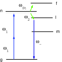
Figure 1: Energy levels and coupled fields.

Levels $m$ and $l$ give the major contribution to the corresponding two-photon quantum pathways, and level $f$ to Stark shift. When analyzing sum-frequency process at $\omega_{+}$, level $l$ is placed above $n$ with the same three-photon detuning. All the fields are assumed pulsed, where the duration of each pulse is much shorter than the shortest relaxation time in the quantum system. Through a time-dependent laser-induced Stark shift of level $n$, i.e., SCRAP, the field $E_{St}$ allows the control of two-photon excitation by the field $E_{1}$. By this process, the entire population of the ground level can be moved to the upper state $n$ by the end of the pulse $E_{1}$. Alternatively, maximum coherence at the two-photon transition $gn$ can be achieved by making the populations of states $g$ and $n$ equal by the end of the pulse $E_{1}$. Furthermore, with a judicious delay of the pulse $E_{2}$, one can achieve maximum nonlinear polarization at the frequency $\omega_{\mp}$ and therefore high conversion efficiency of the visible radiation to the VUV range.

2.1 Equations for interacting electromagnetic fields

The propagation of optical waves in a non-conducting medium is described by the wave equation

$$\nabla^{2}\mathcal{E}-\frac{1}{c^{2}}\frac{\partial^{2}\mathcal{E}}{\partial t^{2}}=\frac{4\pi}{c^{2}}\frac{\partial^{2}\mathcal{P}}{\partial t^{2}},$$ (1)

where $\mathcal{P}$ is the electrical polarization,and we assume the nonlinear medium to be isotropic and all the waves to be identically polarized and to propagate along the $z$-axis:

$$\mathcal{E}_{j}(z,t)=\mathop{\rm Re}\{E_{j}(z,t)\exp[i(\omega_{j}t-k_{i}z)]\},$$

$$\mathcal{P}_{j}(z,t)=\mathop{\rm Re}\{P_{j}(z,t)\exp[i(\omega_{j}t-k^{\prime}_{i}z)]\}.$$ (2)

Here $k_{j}$ is the modulus of a wave vector at frequency $\omega_{j}$, $k^{\prime}_{j}$ is the wave vector of nonlinear polarization at the same frequency, and $E_{j}(z,t)$ and $P_{j}(z,t)$ are slowly-varying envelopes.

Assuming a uniform field distribution over the cross section and taking into account Eqs. (2.1) and $k\approx\omega/c$, one can write Eq. (1) in the approximation of slowly-varying amplitudes as

$$2ik\left(\frac{\partial E}{\partial z}+\frac{1}{c}\frac{\partial E}{\partial t}\right)=-4\pi k^{2}P,$$ (3)

where $P=P^{L}+{P}^{(FWM)}e^{-i\Delta kz}$, and $\Delta k$ is the phase mismatch of the interacting waves. We restrict ourselves to the major process under consideration and assume phase matching to be fulfilled so that $\Delta k=0$. Then by setting $z^{\prime}=z$, $t^{\prime}=t-z/c$ and using

$$\frac{\partial E}{\partial z} = \frac{\partial E}{\partial z^{\prime}}\frac{\partial z^{\prime}}{\partial z}+\frac{\partial E}{\partial t^{\prime}}\frac{\partial t^{\prime}}{\partial z}=\frac{\partial E}{\partial z^{\prime}}-\frac{1}{c}\frac{\partial E}{\partial t^{\prime}},$$

$$\frac{\partial E}{\partial t} = \frac{\partial E}{\partial t^{\prime}}\frac{\partial t^{\prime}}{\partial t}+\frac{\partial E}{\partial z^{\prime}}\frac{\partial z^{\prime}}{\partial t}=\frac{\partial E}{\partial t^{\prime}},$$

we can express Eq. (3) in the form

$${\partial E}/{\partial z^{\prime}}=2\pi ikP.$$ (4)

The polarization $P$ can be calculated with the aid of the density matrix $\rho_{ij}$ as

$$P=N\rho_{ij}d_{ji}+\hbox{c.c.},$$

where N is number density of the resonance atoms, $d_{ji}$ are electro-dipole transition matrix elements, and $\rho_{ij}$ are density matrix components oscillating at the corresponding frequencies. The problem then reduces to calculating the off-diagonal elements of the density matrix.

2.2 Density matrix equations

In the case where the pulse durations of all the interacting fields are much less than any relaxation time in the system, all the relaxation terms may be omitted, and the density matrix equations take the form

$$\dot{\rho}_{mn} = -i\left[G_{mn}\rho_{n}+G_{mg}\rho_{gn}\right],$$

$$\dot{\rho}_{ln} = -i\left[G_{ln}\rho_{n}+G_{lg}\rho_{gn}\right],$$

$$\dot{\rho}_{gl} = i\left[\rho_{gn}G_{nl}+\rho_{g}G_{gl}\right],$$

$$\dot{\rho}_{gm} = i\left[\rho_{gn}G_{nm}+G_{gm}\rho_{g}\right]$$

$$\dot{\rho}_{gn} = -i[G_{gm}\rho_{mn}-G_{mn}\rho_{gm}$$

$$+ G_{gl}\rho_{ln}-G_{ln}\rho_{gl}-G_{fn}\rho_{gf}]$$

$$\dot{\rho}_{n} = 2\mathop{\rm Im}\left[G_{nm}\rho_{mn}+G_{nl}\rho_{ln}+G_{nf}\rho_{fn}\right],$$

$$\dot{\rho}_{nf} = iG_{nf}\rho_{n},\,\dot{\rho}_{gf}=i\rho_{gn}G_{nf},\,\rho_{g}=1-\rho_{n}.$$ (5)

Here $\dot{\rho}_{ij}=d\rho_{ij}/dt$ (hereafter we omit the prime on $z$ and $t$, assuming a transformation to a new coordinate system), $G_{ij}(t)=-d_{ij}E_{k}(t)/2\hbar$ are the coupling Rabi frequencies, and $d_{ij}$ are electric dipole transition momenta. In the coupled equations (2.2), we assume that initially only the lower level $g$ is populated and that the populations of levels $m$, $l$ and $f$ are negligibly small during the entire process. We also neglect photo-ionization. Further, we assume two-photon quasi-resonance $\Omega_{gn}=(2\omega_{1}-\omega_{gn})\ll\omega_{ij}$ and that the conditions for one-photon detunings

$$\Omega_{ij}=(\omega_{k}-\omega_{ij})\gg G_{ij}\gg\tau_{i}^{-1}$$ (6)

are fulfilled, where $\tau_{i}$ is the minimum pulse length.

We look for the solution of the coupled equations in the form

$$\rho_{ij}(t) = r_{ij}(t)\exp\left\{-i\Omega_{ij}t\right\},$$

$$G_{ij}(t) = g_{k}(t)\exp\left\{-i\Omega_{ij}t\right\},$$

$$G_{mn}(t) = ag_{1}(t)\exp\left\{-i(\Omega_{mn}t\right\},$$

where $r(t)$ and $g(t)$ are slowly-varying envelopes, and $a=d_{mn}/d_{gm}$. Then using (6) and $|\dot{r}_{ij}|\ll|\Omega_{ij}r_{ij}|$ for all the off-diagonal elements except $r_{gn}$, we can rewrite the equations (2.2) as

$$r_{mn} = \left[ag_{1}r_{n}+g_{1}^{*}r_{gn}\right]/\Omega_{mn},$$

$$r_{ln} = \left[g_{2}r_{n}+g_{-}^{*}r_{gn}\right]/\Omega_{ln},$$

$$r_{gl} = -\left[r_{gn}g_{2}^{*}+r_{g}g_{-}\right]/\Omega_{gl},$$

$$r_{gm} = -\left[a^{*}g_{1}^{*}r_{gn}+g_{1}r_{g}\right]/\Omega_{gm},$$

$$\dot{r}_{gn} = -i[g_{1}r_{mn}-ag_{1}r_{gm}+g_{-}r_{ln}$$

$$- g_{2}r_{gl}-g_{St}^{*}r_{gf}-\Omega_{gn}r_{gn}],$$

$$\dot{r}_{n} = 2\mathop{\rm Im}\left[a^{*}g_{1}^{*}r_{mn}+g_{2}^{*}r_{ln}+g_{St}r_{fn}\right],$$

$$r_{nf} = -g_{St}r_{n}/\Omega_{nf},\,r_{gf}=-r_{gn}g_{St}/\Omega_{gf},$$

$$r_{g} = 1-r_{n}.$$ (7)

Here $\Omega_{nf}=\omega_{St}-\omega_{nf}$, $\Omega_{gl}=2\omega_{1}-\omega_{2}-\omega_{gl}$, $\Omega_{gf}=2\omega_{1}+\omega_{St}-\omega_{gf}$, etc. After simple algebra, Eqs. (2.2) reduce to

$$\dot{r}_{n} =2\mathop{\rm Im}\left[\left(a^{*}\frac{{g^{*}_{1}}^{2}}{\Omega_{mn}}+\frac{{g_{2}^{*}g_{-}^{*}}}{\Omega_{ln}}\right)r_{gn}\right],$$

$$\dot{r}_{gn} =-i[\left(\Omega_{St}-\Omega_{gn}\right)r_{gn}+g_{gn}r_{n}$$

$$+\frac{ag_{1}^{2}}{\Omega_{gm}}+\frac{g_{2}g_{-}}{\Omega_{gl}}],$$ (8)

where

$$g_{gn} =\left(\frac{ag_{1}^{2}}{\Omega_{mn}}+\frac{g_{2}g_{-}}{\Omega_{ln}}-\frac{ag_{1}^{2}}{\Omega_{gm}}-\frac{g_{2}g_{-}}{\Omega_{gl}}\right),$$

$$\Omega_{St} =\frac{|g_{-}|^{2}}{\Omega_{ln}}+\frac{|g_{St}|^{2}}{\Omega_{gf}}+\frac{|g_{1}|^{2}}{\Omega_{mn}}+\frac{a^{2}|g_{1}|^{2}}{\Omega_{gm}}+\frac{|g_{2}|^{2}}{\Omega_{gl}}.$$ (9)

2.2.1 Generalized two-level scheme

In the more general case of multi-level system a sum over all intermediate states $m$ and $l$ must be taken. In view of that, we introduce the values

$$r_{1} =-2\frac{ag_{1}^{2}}{\Omega_{gm}}=\gamma_{1}E_{1}^{2},\,s=\frac{|g_{St}|^{2}}{\Omega_{nf}}=\beta_{S}|E_{St}|^{2},$$

$$s_{1} =\left(\frac{a^{2}}{\Omega_{gm}}+\frac{1}{\Omega_{mn}}\right)|g_{1}|^{2}=\beta|r_{1}|=\beta_{1}|E_{1}|^{2},$$

$$r_{2} =-2\frac{g_{2}g_{-}}{\Omega_{gl}}=\gamma_{2}E_{2}E_{-},\,s_{2}=\frac{|g_{2}|^{2}}{\Omega_{gl}}=\beta_{2}|E_{2}|^{2},$$

$$s_{-} =\frac{|g_{-}|^{2}}{\Omega_{ln}}=\beta_{-}|E_{-}|^{2},$$ (10)

where $\gamma_{i}$ and $\beta_{i}$ are polarizabilities depending on specific atoms and contributing quantum transitions. In the vicinity of a two-photon resonance $\Omega_{mn}\approx-\Omega_{gm}$ and $\Omega_{ln}\approx-\Omega_{gl}$. Then Eqs. (2.2) take the form:

$$\dot{r}_{n} =\mathop{\rm Im}\left[\left(r_{1}^{*}+r_{2}^{*}\right)r_{gn}\right],$$

$$\dot{r}_{gn} =-i\left(\Omega_{St}-\Omega_{gn}\right)r_{gn}$$

$$-i\left(r_{1}+r_{2}\right)\left(r_{n}-1/2\right),$$ (11)

where

$$\Omega_{St}=s+s_{1}+s_{2}+s_{-}.$$ (12)

It is seen from Eqs. (2.2) that $\Omega_{St}$ is the laser-induced shift of the two-photon resonance.

2.3 Evolution of Rabi frequencies along the medium

We assume that one-photon Rabi frequencies of all the fields vary in time as

$$g_{i}(t)=g_{i0}\exp\{-(t-\Delta\tau_{i})^{2}/2\tau_{i}^{2}\}.$$ (13)

Here $2\tau_{i}$ is the width of the $i$-th pulse (at $e^{-1}$ of the power maximum), and $\Delta\tau_{i}$ is the time delay of the $i$-th pulse relative to $t=0$. The pulse widths are assumed to be much shorter than the relaxation rates of the system. We also assume that the spectral width of the pulse $E_{1}$ is much greater than the Doppler width of the transition $gn$, and are replaced Eq. (4) by the equations for the corresponding Rabi frequencies,

$${d\,g_{1}}/{d\,z} = -i\pi\hbar^{-1}k_{1}|d_{gm}|^{2}N(r_{gm}+a^{*}r_{mn})$$

$$= -i\alpha_{1}(r_{gm}+a^{*}r_{mn}),$$

$${d\,g_{2}}/{d\,z} = -i\alpha_{2}r_{ln},\quad{d\,g_{-}}/{d\,z}=-i\alpha_{-}r_{gl},$$

where $\alpha_{1,2,-}$ are resonant frequency-integrated absorption indices at the corresponding transitions for broadband probe radiations, with all other fields turned off. Then by scaling the medium length to the absorption length $\alpha_{-}^{-1}$, which is a characteristic parameter for the given medium that can be measured independently, we obtain

$${d\,g_{1}}/{d\xi} = -iK_{1}(r_{gm}+a^{*}r_{mn}),$$

$${d\,g_{2}}/{d\xi} = -iK_{2}r_{ln},$$

$${d\,g_{-}}/{d\xi} = -ir_{gl},$$ (14)

where

$$K_{1} = (k_{1}|d_{gm}|^{2})/(k_{-}|d_{gl}|^{2})$$

$$= (k_{1}\omega_{gl}|f_{gm}|)/(k_{-}\omega_{gm}|f_{gl}|),$$

$$K_{2} = (k_{2}|d_{ln}|^{2})/(k_{-}|d_{gl}|^{2})$$

$$= (k_{2}\omega_{gl}|f_{ln}|)/(k_{-}\omega_{ln}|f_{gl}|),$$

$$\xi = \alpha_{-}z.$$ (15)

In the above consideration we ignored Doppler effects, which is possible, for example, in atomic beams. In the case of warm gas, the solution of the equations must be averaged over a Maxwell velocity distribution of atoms. However, Doppler effects do not contribute much if the equivalent spectral width of the pulses or/and all detunings are greater or comparable with the corresponding resonance Doppler HWHM.

3 Numerical simulation of SCRAP and maximum coherence in a generalized two-level scheme

For further numerical simulations we introduce the parameters $\delta=\Omega_{gn}\tau_{1}$, $S=s_{0}\tau_{1}$, $R=r_{10}\tau_{1}$, $T=t/\tau_{1}$ and $\delta\tau=\Delta\tau/\tau_{1}$, which are the detuning and maximum dynamic shift of the resonance scaled to the spectral width of the pulse $E_{1}$ (Eqs. (13)), number of Rabi oscillations during the pulse duration $\tau_{1}$, and time and pulse shifts scaled to the duration of this pulse. In this subsection we analyze the dynamics of population transfer and induced coherence, assuming $g_{2}=0$ and the dynamic self-shift of the resonance to be negligible ($\beta=0$). Then the equations (2.2.1) describe laser-induced oscillations in a two-level system controlled by the auxiliary Stark field. The corresponding level scheme and radiative coupling are shown in Fig. 2.

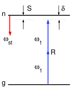
Figure 2: Generalized two-level scheme and radiative couplings.

3.1 Oscillations induced by a rectangular pulse

First, we simulate the well-known dynamics induced by pulses of rectangular shape and duration $\tau$ at $\Omega_{gn}=\Omega_{St}$ ($\pi/2$, $\pi$ and $2\pi$ pulses). Then the equations (2.2.1) take the form:

$$\dot{r}_{gn}=-ir_{1}(r_{n}-1/2),\quad\ddot{r}_{n}=-|r_{1}|^{2}(r_{n}-1/2).$$ (16)

Equation (16) describes induced oscillations with the two-photon Rabi frequency $|r_{1}|$. The coherence $r_{gn}$ reaches its maximum ($\dot{r}_{gn}=0$) at $r_{n}=1/2$. Then $r_{g}=1-r_{n}=1/2$ too, and $r_{gn}$, which is product of the corresponding probability amplitudes, reaches its maximum $|r_{gn}|=1/2$ as well.

At $\Omega=\Omega_{gn}-\Omega_{St}=0$ and $t=\pi/2|r_{1}|$, half of the population of the ground state transfers to the excited state, and the amplitude of the polarization oscillations $|r_{gn}|$ reaches its maximum. At $t=\pi/|r_{1}|$ the entire population of the ground state is transferred to the excited state. At $t=3\pi/2|r_{1}|$ the coherence again reaches its maximum, and at $t=2\pi/|r_{1}|$ the system returns to its initial state. Such oscillations are illustrated in Fig. 3. Deviation from resonance leads to increased frequency and decreased amplitude of the oscillations for the level populations (Fig. 3 (left)), and the instant when maximum coherence is reached will vary. However, the maximum value of coherence, which is 0.5, is not achievable if the population of the upper level does not reach 0.5. (Fig. 3 (right)).

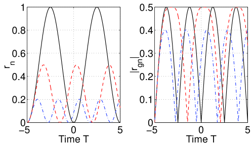
Figure 3: Dependence of the population $r_{n}$ and coherence $|r_{gn}|$ on time $T$ in a generalized two-level scheme with excitation by a rectangular pulse at various deviations from resonance $\Omega_{gn}$. Time is scaled to the arbitrary value $\tau$ which is much less then any relaxation rate in the system. The coupling Rabi frequency $R=r_{1}\tau=2\pi/5$, and $\delta=\Omega_{gn}\tau$ are scaled to $\tau^{-1}$. Solid line – $\delta=0$, dashed – $\delta=1.259$, dash-dotted – $\delta=2.5$.

3.2 Dynamics of generalized two-level system driven by Gaussian pulses

In further analysis we shall account for the differences which appear for the pulses of Gaussian shape (Eq. (13)). This leads to variation in time of the two-photon Rabi frequency and Stark shifts as:

$$r_{i}(t)=r_{i0}\exp\left[-(t-\Delta\tau_{i})^{2}/\tau_{i}^{2}\right],$$

$$s(t)=s_{0}\exp\left[-(t-\Delta\tau_{St})^{2}/\tau_{St}^{2}\right],$$

$$s_{i}(t)=s_{i0}\exp\left[-(t-\Delta\tau_{i})^{2}/\tau_{i}^{2}\right].$$ (17)

Hereafter, we will scale a static deviation from the two-photon resonance $\Omega_{gn}$, amplitudes of the dynamic resonance shift $s_{0}$ and Rabi frequency $r_{10}$ to the spectral width $\tau_{1}^{-1}$, and delay of the Stark pulse $\Delta\tau$ and time $t$ to the duration of the excitation pulse $\tau_{1}$: $\delta=\Omega_{gn}\tau_{1}$, $S=s_{0}\tau_{1}$, $R=r_{10}\tau_{1}$, $\delta\tau=\Delta\tau/\tau_{1}$, $T=t/\tau_{1}$.

3.2.1 Persistent maximum coherence created by Gaussian pulses at negligible dynamic self-shift of the resonance

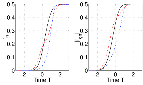
Figure 4: Population $r_{n}$ and persistent maximum coherence $|r_{gn}|$ controlled by the dynamic Stark shift at various static deviations from the two-photon-resonance and moderate two-photon Rabi frequencies. The Stark shift produced by the two-photon excitation is ignored. The duration of the control Gaussian Stark-shift pulse is $\tau_{St}/\tau_{1}=1.6$. Solid plot — $\delta=0$, $S=0$, $R=0.886$; dashed — $\delta=5$, $S=7.4$, $R=3.18$, $\delta\tau=1.8$; dash-dotted — $\delta=20$, $S=23$, $R=3.48$, $\delta\tau=1.34$.

In the case under consideration in this sub-subsection ($\beta=0$), the principal contribution to $\Omega_{St}$ is determined by $E_{St}$, such that the entire Stark shift depends on time as

$$\Omega_{St}(t) = s_{0}\exp\left[-(t-\Delta\tau_{St})^{2}/\tau_{St}^{2}\right].$$ (18)

We choose the intensity and frequency detuning of the Stark field such that the Stark shift $\Omega_{St}$ can compensate for the two-photon detuning $\Omega_{gn}$. In order to provide a dynamic two-photon resonance, the requirement $|s_{0}|>|\Omega_{gn}|$ must be fulfilled. Then the resonance condition is met at two instants of time:

$$t_{1,2}=\Delta\tau_{St}\mp\tau_{St}\sqrt{\ln({s_{0}}/{\Omega_{gn})}}.$$ (19)

By a proper choice of the field parameters, one can provide first passage of the two-photon resonance at such an instant that the value of the two-photon Rabi frequency ensures a $\pi/2$ process over the period of passage through the resonance. For example, if the first instant of the crossing of the resonance is $t_{1}=0$ and the second one is $t_{2}=2\Delta\tau_{St}$, then the requirement is:

$$\Omega_{gn}=s_{0}\exp(-\Delta\tau_{St}^{2}/\tau_{St}^{2})$$ (20)

A numerical analysis of corresponding feasibilities of creation of persistent maximum coherence is presented in Fig. 4. Figure 4 (solid) illustrates the maximum coherence generated by the resonance $\pi/2$ pulse with the Stark field turned off. Figures 4 (dash and dash-dotted) show such opportunities realized with the aid of the Stark field at various deviations of excitation from the two-photon resonance. The Stark shift at the front of the pulse is adjusted to compensate for the static deviation at the instant when the excitation is around its maximum values, while the Rabi frequency is about the magnitude required to transfer half of the population of the ground state to the excited one during the period of passage through the resonance. Due to the appropriately selected pulse shift, the Rabi frequency is too small for the population to return to the ground state while passing through the resonance at the rear of the Stark pulse.

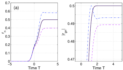
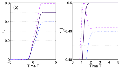
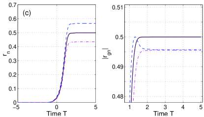
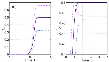
Figure 5: Robustness of maximum coherence created with the Gaussian pulses of two-photon excitation and Stark shift of the resonance, while the dynamic self-shift of the resonance is neglected ($\beta=0$), and $\tau_{St}/\tau_{1}=1.6$. (a) – $\delta=5$, $R=3.18$, $\delta\tau=1.8$, solid – $S=7.4$, dashed – $S=6.7$, dash-dotted – $S=8.1$; (b) – $S=7.4$, $R=3.18$, $\delta\tau=1.8$, solid line – $\delta=5$, dashed – $\delta=4.5$, dash-dotted – $\delta=5.5$; (c) – $S=23$, $\delta=20$, $\delta\tau=1.34$, solid – $R=3.48$, dashed – $R=3.85$, dash-dotted – $R=3.15$; (d) – $R=3.48$, $S=23$, $\delta=20$, solid – $\delta\tau=1.34$, dashed – $\delta\tau=1.2$, dash-dotted – $\delta\tau=1.5$.

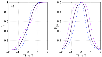
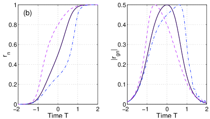
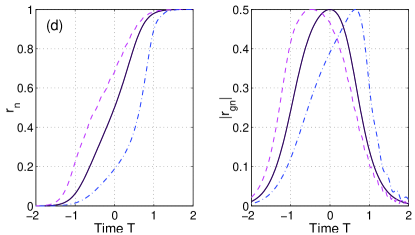
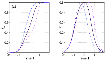
Figure 6: Rapid adiabatic passage assisted by Stark-chirp and two-photon coherence, while the dynamic self-shift of the resonance is ignored ($\beta=0$), and $\tau_{St}/\tau_{1}=1.6$. (a) – $\delta=24$, $S=75$, $\delta\tau=1.7$, solid line – $R=30$, dashed – $R=15$, dash-dotted – $R=60$; (b) – $S=75$, $R=30$, $\delta=24$, solid – $\delta\tau=1.7$, dashed – $\delta\tau=1.1$, dash-dotted – $\delta\tau=2.3$; (c) – $\delta=24$, $R=30$, $\delta\tau=1.7$, solid line – $S=75$, dashed – $S=50$, dash-dotted – $S=150$; (d) – $R=30$, $S=75$, $\delta\tau=1.7$, solid line – $\delta=24$, dashed – $\delta=12$, dash-dotted – $\delta=48$.

The results of simulations depicted in Fig. 5 show that the variation of the given radiative parameters about 10% of their optimum values leads to comparable change of the population transfer. As an important outcome, it demonstrates substantially less change of the coherence amplitude and therefore attests to its robustness. This is due to the fact that the product of the probability amplitudes of the ground and excited states changes less than the square modulus of probability amplitude of the upper state.

3.2.2 Stark-chirped rapid adiabatic passage and transient maximum coherence

As indicated above, the key idea of SCRAP [25] is to enhance the transition probability at $t_{1}$ and to minimize it at $t_{2}$ (see Eq. (19)), which is possible if the evolution is adiabatic at $t_{1}$ and diabatic at $t_{2}$. Creation of maximum coherence is ensured in the process of rapid adiabatic passage of the entire population from the ground to excited state, where maximum coherence is always induced at instants when populations of the level becomes equal. Figure 6 presents such behavior. It shows robustness of such passage, although the instants when coherence reaches its maximum may change substantially.

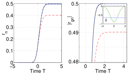
Figure 7: Effect of dynamic self-shift of two-photon resonance $s_{1}=\beta R$ on creation of persistent maximum coherence. $S=0$. $R=0.886$, solid line – $\beta=0$, $\delta=0$ ($\pi/2$-pulse), dash-dotted – $\beta=-1$, $\delta=0$, dashed (overlaps the solid one) – $\beta=-1$, $\delta=-0.65$. Insert – dependence of the dynamic self-shift of the two-photon resonance $s_{1}$ on time. The static deviation from the resonance is marked by the straight line.

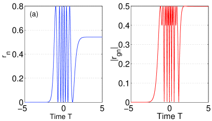
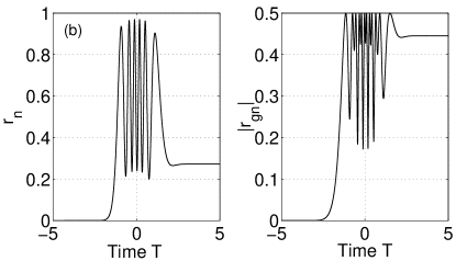
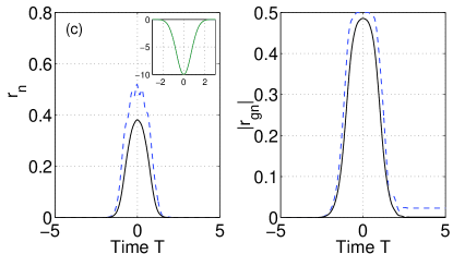
Figure 8: Population $r_{n}$ and coherence $|r_{gn}|$ determined by the dynamic shift of the two-photon resonance driven both by resonant excitation $s_{1}=\beta R$ and by an auxiliary Stark-shift field $s$. $R=20$, $S=0$, $\beta=-0.5$; (a)– $\delta=0$, (b)– $\delta=-3$, (c) – dashed line – $\delta=-10$, solid – $\delta=-15$. Insert – dependence of the dynamic shift $s_{1}$ induced by two-photon excitation (dashed line) and by two-photon excitation in cooperation with the auxiliary Stark field $s_{1}+s$ (solid line).

3.2.3 Maximum coherence and rapid adiabatic passage controlled by the dynamic shift of a two-photon resonance produced by both fundamental and Stark Gaussian pulses

In a multi-level system with appreciable difference between the principal quantum numbers of the ground and excited states, two-photon excitation may substantially contribute to the dynamic shift of a resonance. This makes transient effects and consequently the choice of the parameters ensuring maximum coherence and rapid adiabatic passage more complicated. Figure 7 presents such behavior, where the solid line shows feasibility to generate persistent maximum coherence in the absence of dynamic shift of the resonance (a $\pi/2$ pulse). It is seen that even a relatively small self-induced dynamic shift of the two-photon resonance may substantially change the time-behavior of the system (dash-dot plot). However, persistent maximum coherence can be restored through an appropriately chosen static deviation from the resonance provided that the Rabi frequency is around the value corresponding to a $\pi/2$-pulse.

Under larger intensities of two-photon excitation, the dynamics of the system controlled by the dynamic self-shift becomes more complicated, so that generation of persistent coherence without the means of independent control of the shift with an auxiliary pulse may become impossible (Fig. 8).

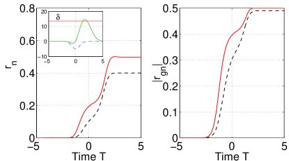
Figure 9: Creation of persistent maximum coherence controlled by appropriate static deviation from resonance and by appropriate delay of he auxiliary Stark-shift pulse in the system experiencing the dynamic self-shift of the two-photon resonance. $s_{1}=\beta R$, $\beta=-0.5$, $S=15$, $\delta=13.65$, $\delta\tau=1.6$; dashed line – $R=15$, solid – $R=30$. Insert – dependence of the dynamic shift $s_{1}$ induced by two-photon excitation (dashed line) and by two-photon excitation in cooperation with the auxiliary Stark field $s_{1}+s$ (solid line). The static deviation from the resonance is marked by the straight line.

Indeed, independent control of the dynamic shift of the two-photon resonance with the aid of the auxiliary Stark-shift pulse, and based on the above discussed algorithm, ensures creation of persistent maximum two-photon coherence (Fig. 9).

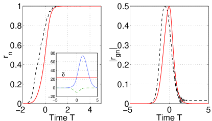
Figure 10: Persistent Stark-chirp-assisted rapid adiabatic passage controlled by the appropriately delayed pulses and by static deviation from resonance in the system experiencing a dynamic self-shift of the two-photon resonance. $s_{1}=\beta R$, $\beta=-0.5$, $S=75$, $R=20$, $\delta\tau=1.4$; dashed line – $\delta=10$, solid – $\delta=24$. Insert – dependence of the dynamic shift $s_{1}$ induced by two-photon excitation (dashed line) and by two-photon excitation in cooperation with the auxiliary Stark field $s_{1}+s$ (solid). the static deviation from the resonance is marked by the straight line.

Figure 10 illustrates similar opportunities for transient maximum coherence generated through persistent transfer of the entire population of ground state to the upper state (SCRAP).

4 Dynamics of energy level populations, four-wave mixing at maximum coherence, and VUV generation in Hg vapors

In this section, we apply our theory for simulating the features of two-photon resonant FWM controlled by SCRAP with the aid of a numerical model appropriate for quantum transitions in Hg. Then the energy levels depicted in (Fig. 1) are attributed to those of $Hg$ as follows: $g$ – $6s^{2}\,{}^{1}S_{0}$, $n$ – $8s\,^{1}S_{0}$, $m$ – $6p\,^{1}P_{1}$, $l$ – $6p\,^{1}P_{1}$, $f$ – $7p\,^{1}P_{1}$, and the laser parameters are similar to those described in Ref. [25]: $\lambda_{1}=268.8$ nm, $\lambda_{St}=1064$ nm, $\lambda=532$ nm, $\tau_{1}=3$ ns. Then $\lambda_{-}=179.8$ nm, $\lambda_{+}=107.3$ nm, $\delta_{nf}\sim\delta=8.9\times 10^{3}$, $\delta_{nl}=-2.2\times 10^{4}$ and $\delta_{gm}=-2.4\times 10^{5}$ (all detunings are scaled to $\tau_{1}^{-1}$). The parameters $a$ and $K_{j}$ are taken as $a=0.345$, $K_{-}=1,K_{2}=0.04,K_{1}=0.67$. We have assumed that other levels, which are not depicted here, do not contribute substantially to the coupling. The other pulse durations are chosen as: $\tau_{2}=\tau_{1}$, $\tau_{St}/\tau_{1}=1.6$. The delay between all these pulses can be varied. We introduce the parameters $G_{i}=|g_{i}|\tau_{1}/2\pi$ and $Z=\xi\tau_{1}/2\pi$, which denote reduced by $2\pi$ the number of Rabi oscillations during the pulse $E_{1}$ and the medium length scaled to the resonant absorption length at the transition $gl$ for the nonmonochromatic radiation with the spectral width $\tau_{1}^{-1}$. The results of the simulations are presented below.

As outlined above, in order to achieve a transfer efficiency close to unity, one must fulfill the adiabatic condition described in Ref. [25]). Through a proper choice of $G_{01}$, $G_{0st}$, static detuning $\delta$ and pulse delay $\delta\tau_{st}$, we can ensure various values and evolution in time of the populations and coherence at the entrance to the medium. Figures 11-14 demonstrate the possible dynamics leading either to maximum population transfer or to equal populations and maximum coherence. These pictures (along with Fig. 6) illustrate the robustness of these processes, regardless of the significant change in some of the parameters.

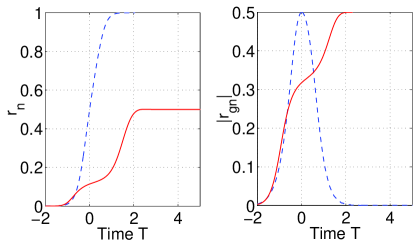
Figure 11: Dependence of the population $r_{n}$ and coherence $|r_{gn}|$ on time at the entrance to the medium. $G_{01}=910$, $G_{0st}=325$. Solid line – $\delta=0.5$, $\delta\tau_{st}=-3$, dashed – $\delta=5.6$, $\delta\tau_{st}=2$. Other parameters are given above.

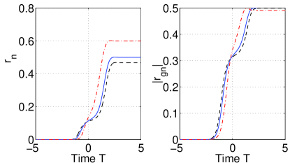
Figure 12: Dependence of the population $r_{n}$ and coherence $|r_{gn}|$ on time at the entrance to the medium. $G_{0st}=325$, $\delta=0.5$, $\delta\tau_{st}=-3$. Solid line – $G_{01}=910$, dashed – $G_{01}=1173$, dash-dotted – $G_{01}=525$.

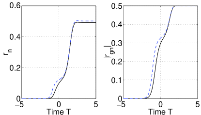
Figure 13: Dependence of the population $r_{n}$ and coherence $|r_{gn}|$ on time at the entrance to the medium. $G_{01}=910$, $\delta=0.5$, $\delta\tau_{st}=-3$. Solid line – $G_{0st}=461$, dashed – $G_{0st}=266$.

Figure 14: Dependence of the population $r_{n}$ and coherence $|r_{gn}|$ on time at the entrance to the medium. $G_{01}=910$, $G_{0st}=325$, $\delta=0.5$. Solid line – $\delta\tau_{st}=-4$, dashed – $\delta\tau_{st}=-3$, dash-dotted – $\delta\tau_{st}=-2$.

The generated radiation depends strongly on the dynamics of the coherence and on the delay at which the pulse $G_{2}$ to be converted is applied. For the cases depicted in Fig. 11, one can choose either a relatively short interval, when populations of the levels $n$ and $g$ becomes equal and the coherence amplitude reaches its maximum, or a ’plateau’ with lower but almost constant amplitude of the two-photon coherence $|r_{gn}|$ in time. Furthermore, in our simulations, if it is not indicated otherwise, we assume that $G_{0st}=325$ and at the entrance of the Hg cell, $G_{01}=910$ (which corresponds to $R=15$, $S=75$), and the amplitude of the pulse $G_{2}$ is chosen to be non-perturbatively small ($G_{20}=1.6\times 10^{-2}$). The delay of the pulse $G_{2}$ is set as $\delta\tau_{2}=5$, so that this pulse overlaps the plateau in the time dependence of the coherence $|r_{gn}|$ at the entrance to the medium (Fig. 11, solid line), or $\delta\tau_{2}=0$, so that the maximum of the convertible pulse coincides with the maximum of the time dependence of the coherence (Fig. 11, dashed line).

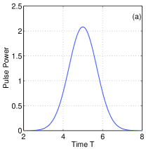
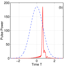
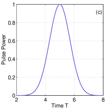
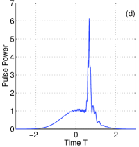
Figure 15: Shapes of the generated $|G_{-}/G_{02}|^{2}$ (a,b) and amplified $|G_{2}/G_{02}|^{2}$ (c,d) pulses at $Z=3\times 10^{6}$. (a) and (c) correspond to the plots in Fig. 11 (solid line), with $\delta\tau_{2}=5$, and (b) and (d) to the plots at Fig. 11 (dashed line) with $\delta\tau_{2}=0$. The dashed line in plot (b) is the input pulse scaled to the maximum of the output one. For the plot (c), the shapes of the input and output pulses are similar.

Figures 15(a-d) computed for difference-frequency processes show that the shape of the generated and convertible pulses may substantially vary along the medium, subject to the coherence dynamics and the time delay $\delta\tau$ at the entrance of the medium. It is seen that if the pulse $G_{2}$ overlaps the plateau of the time dependence of $|r_{gn}|$, there is no significant transformation of the pulse shape along the medium (the corresponding plots in Fig. 15(c) coincide). On the contrary, if the maximum coherence is reached in a transient regime, and the maximum of the pulse $G_{2}$ coincides with the instant when the populations of the levels $r_{g}$ and $r_{n}$ become equal at the entrance to the medium, the change of pulse shapes is most significant (Fig. 15(b,d)). In the first case, all the parts of the pulse $G_{2}$ are converted homogeneously. In the second case, the wings of the pulse $G_{2}$ are not converted and enhanced since the shape of the pulse $|r_{gn}|$ is substantially narrower than that of $G_{2}$. This leads to a sharpening of both the generated and convertible (i.e., amplified) pulses. The shape of the excitation pulse may substantially change along the medium too, although its energy has practically no change (see Fig. 16).

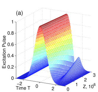
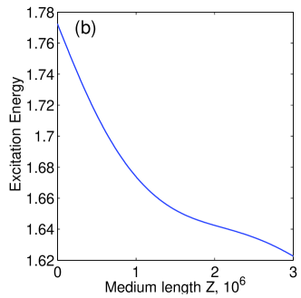
Figure 16: Evolution of the shape of the pulse $|G_{1}/G_{01}|^{2}$ (a) and its energy $\int|G_{1}/G_{01}|^{2}dt$ (b) along the medium. $\delta=0.5$, $\delta\tau_{st}=-3$.

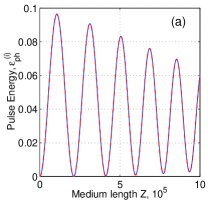
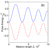
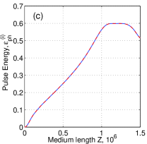
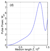
Figure 17: Evolution the pulse energy $\varepsilon_{ph}$ of the convertible and generated fields, scaled to the initial number of photons at convertible frequency $\omega_{2}$ along the medium. (a-c). (a) – down-conversion $\omega_{-}=2\omega_{1}-\omega_{2}$ and (b) – up-conversion $\omega_{+}=2\omega_{1}+\omega_{2}$, both correspond to the plots at Fig. 11 (solid line) whith $\delta\tau_{2}=5$, and (c,d) to down conversion, which correspond to the plots at Fig. 11 (dashed line) whith $\delta\tau_{2}=0$. (c) – energy $\epsilon_{ph}$, (d) – peak pulse power $W_{ph}^{max}$. For up-conversion (b) plots for generated (solid line) and for convertible (dashed) fields are different, for down-conversion (a,c,d) their behavior is similar.

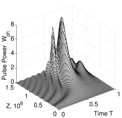
Figure 18: Evolution of the pulse shape $W_{ph}(T)$ of the generated and convertible radiations (coincide), with all parameters the same as in Fig. 17(c).

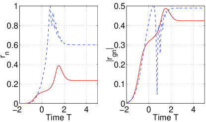
Figure 19: Evolution in time of the population $r_{n}$ and coherence $|r_{gn}|$ at the medium length $Z=1\times 10^{6}$. $G_{01}=910$, $G_{0st}=325$. Solid line – $\delta=0.5$, $\delta\tau_{st}=-3$, dashed – $\delta=5.6$, $\delta\tau_{st}=2$.

Figure 17(a-c) shows the dependencies of the pulse energy

$$\varepsilon_{ph}^{(i)}=\frac{\int|G_{i}(\tau)|^{2}\,d\tau-\int|G_{0i}(\tau)|^{2}\,d\tau}{\int|G_{02}(\tau)|^{2}\,d\tau}\cdot\frac{\omega_{2}|d_{ln}|^{2}}{\omega_{i}|d_{i}|^{2}},$$ (21)

and Figure 17(d) the pulse power at the instances when it reaches its maximum

$$W_{ph}^{(i)}=\frac{|G_{i}(\tau)|_{max}^{2}-|G_{0i}(\tau)|_{max}^{2}}{|G_{02}(\tau)|_{max}^{2}}\cdot\frac{\omega_{2}|d_{ln}|^{2}}{\omega_{i}|d_{i}|^{2}},$$ (22)

along the medium. Both are scaled to the corresponding value for the convertible field $E_{2}$ at the entrance of the medium. The plots (a,b) are computed for the case when, at the entrance to the media, the pulse $E_{2}$ overlaps the plateau in the time dependence of the coherence $|r_{gn}|$. The simulations show that in this case there is no difference between the plots for energy and power. On the contrary, in the case when the second pulse overlaps maximum of the transient coherence, the difference between energy and power becomes significant (Fig. 17(c,d)), because pulse shapes experience change along the medium (Fig. 18).

The figures show that the evolution of the fields along the medium is strongly determined by the coherent nonlinear coupling. The difference in evolution of the field $E_{2}$ in plots (a,b) is due to the fact that the field $E_{2}$ is enhanced in the difference-frequency mixing process and, by contrast, depletes during the course of the sum-mixing process. The simulation reveals a substantial difference in the evolution, depending on such coupling parameters at the entrance to the medium, like the static detuning and delays between pulses, which control the coherence in time and along the medium. The maximum achieved amplitude of the generated field may change by several times, and the conversion efficiency for the sum-frequency process may approach unity. The figures prove the feasibilities of substantial (by more than several tens times) improvement of the conversion efficiency by a judicious fit of the parameters at the medium entrance. Since the pulse shape of the driving field $E_{1}$ varies along the medium, consequently, the populations $r_{g}$, $r_{n}$, as well as the coherence $r_{gn}$, vary along the medium too. Therefore, the system being optimally prepared at the entrance (Fig. 11) may evolve to less optimum along the medium (Fig. 19, solid line). Alternatively, this can be properly adjusted so that the generated radiation may grow over a greater length, and the conversion efficiency may become substantially larger as well. Consequently, conversion efficiency of the input green radiation to VUV range, which is greater than unity, becomes possible for difference-frequency process.

Simulations show that, besides other parameters, the actual power, energy and photon conversion efficiencies are strongly dependent on the strengths of the involved transitions and on their ratios (parameters $a$ and $K_{j}$). Figure 20 displays the same results as in Fig. 17(a) except that the ratio $|d_{ln}/d_{gl}|=0.35$ is changed for 1.1. Consequently, the parameter $K_{2}$ changes from 0.04 to 0.4. The squared modulus of the nonlinear polarization, which determines the FWM generated power, is proportional to the product of squared modules of these transition electric dipole matrix elements. Consequently, the output generated power increases as well. (The squared modulus of the output Rabi frequency, plotted in some of the graphs, increases by several orders even at the same output power.) Therefore, the major features of the generation, optimum conditions and and maximum output power depend on the specific quantum system employed.

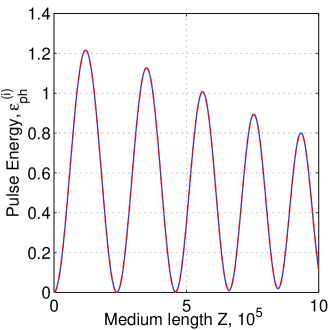
Figure 20: Same as in Fig.17(a), but $|d_{ln}/d_{gl}|=1.1$ ($K_{2}=0.4$).

The characteristic absorption length $z_{0}=(\alpha_{-}\tau_{1}/2\pi)^{-1}$ for Hg and the medium lengths corresponding to Figs. 17-20 are estimated as follows: The frequency-integrated absorption index is calculated as $\alpha_{-}=\pi\Gamma_{gl}\alpha_{0-}=\lambda_{s}^{2}g_{l}A_{lg}N/4$, where $\alpha_{0-}$ is the resonant value of the absorption index for the monochromatic radiation, $\Gamma_{gl}$ is the half-width of the resonance, $A_{lg}$ is the spontaneous relaxation rate at the transition, $g_{l}$ is the degeneration factor for level $l$, and $N$ is the Hg number density. The oscillator strength for the Hg transitions $6s^{2}\,{}^{1}S_{0}-6p\,{}^{1}P_{1}$ ($\lambda=184.9$ nm) is $f\approx 0.96$. Since $A_{lg}=0.67g_{g}f_{lg}/g_{l}\lambda_{lg}^{2},$ where $\lambda$ is given in cm, one obtains $\alpha_{-}=(0.67g_{g}f_{lg}N/4)$ cm^-1c^-1, and for $\tau=3$ ns, and $N=10^{16}$ cm^-3, an estimate gives $\alpha_{s}\tau_{1}/2\pi\approx 7.6\times 10^{5}\hbox{ cm}^{-1}$. Therefore, $Z=10^{6}$ corresponds to a medium length of about 1.3 cm.

5 Conclusions

We have presented an investigation of specific features of four-wave mixing of delayed short pulses in two-photon resonant media, controlled by a dynamic Stark shift of the resonance. Through numerical simulation, we have analyzed different regimes of preparation of laser-induced maximum coherence and its implementation for frequency conversion. We have shown that by a proper choice of the time delays between the interacting laser pulses, the conversion efficiencies may be enhanced by several orders of magnitude with respect to conventional four-wave mixing. The results indicate the feasibility of this technique to generate strong tunable vacuum-ultraviolet radiation.

References

- [1] Wallenstein, R., 1982, Laser Optoelektr. 3, 29.
- [2] Arkhipkin, V. G., and Popov, A. K., 1987, Soviet Physics: Uspekhi 30, 952 [translated from Uspekhi Fizicheckikh Nauk 153, 423 (1987), which is a short version of the book Arkhipkin, V. G., and Popov, A. K., 1987, Nonlinear Light Conversion in Gases, Siberian Branch of Nauka Press, Novosibirsk (in Russian)].
- [3] Heller, Yu. I., and Popov, A. K., 1981, Laser-Induction of Nonlinear Resonances in Continuous Spectra, Siberian Branch of Nauka Press, Novosibirsk, 159 (in Russian); [translated into English, 1985, J. Sov. Laser Res., c/b Consultants Bureau, Plenum, New York, USA, 1985, 6, 1].
- [4] Popov, A. K., and Rautian, S. G., 1996, in (” Coherent Phenomena and Amplification without Inversion,” ed. by Andreev, A. V., Kocharovskaya, O., and Mandel, P., SPIE Proc. 2798, 49.
- [5] Popov, A. K., 1996, Bull. Russian Acad. Sci. (Physics) 60, 927 [translated by Allerton Press, New York, 1996, Izvestiya RAN, seriya Fizika 60, 99.] (http://xxx.lanl.gov/ABS/QUANT-PH/0005108).
- [6] Popov, A. K., 1998, SPIE Proc. 3485, 252.
- [7] Harris, S. E., Field, J. E., Imamoglu, A., 1990, Phys. Rev. Lett. 64, 1107.
- [8] Marangos, J. P., 1998, J. Mod. Opt. 45, 471.
- [9] Arimondo, E., 1996, Prog. Opt. 35, 259.
- [10] Zhang, G. Z., Hakuta, K., and Stoicheff, B. P., 1993, Phys. Rev. Lett. 71, 3099.
- [11] Dorman, C., Kucukkara I., and Marangos, J. P., Phys.Rev A, 2000, 61, 013802.
- [12] Dorman, C., Kucukkara, I., and Marangos, J.P., 2000, Opt. Commun. 180, 263.
- [13] Hemmer, P., Katz, D., Donoghue, J., Cronin-Golomb, M., Shahriar M., and Kumar, P., 1995, Opt.Lett. 20, 928.
- [14] Jain, M., Xia, H., Yin, G. Y., Merriam, A. J., and Harris, S. E., 1996, Phys. Rev. Lett. 77, 4326.
- [15] Arkhipkin, V. G., Myslivets, S. A., Manushkin, D. V., and Popov, A. K., 1998, J. Quantum Electron. 28, 637, [translated from: 1998, Kvantovaya Elektronika 25, 655 (1998)]; ibid,. 1998, SPIE Proc. 3485, 252.
- [16] Popov, A. K., Bayev, A. S., George, T. F., and Shalaev, V. M., 2000, Europ. Phys. J. D - EPJdirect D1, 1 (http://link.springer.de/link /service/journals/10105/tocs/t0002d.htm).
- [17] Harris, S. E., Yin, G. Y.,Jain, M., Xia, H., and Merriam, A. J., 1997, Phil. Trans. Roy. Soc. London (Math., Phys. Eng. Series) 355, 2291.
- [18] Lukin, M. D., Hemmer, P. R., Löffler, M., and Scully, M. O., 1998, Phys. Rev. Lett. 81, 2675.
- [19] Hakuta, K., Suzuki, M., Katsuragawa, M., and Li, J. Z., 1997, Phys. Rev. Lett. 79, 209.
- [20] Merriam, A., Sharpe, S. J., Xia, H., Manuszak, D., Yin, G. Y., and Harris, S. E., 1999, Opt. Lett. 24, 625.
- [21] Vitanov, N., Halfmann, T., Shore, B. W., and Bergmann, K., 2001, Ann. Rev. Phys. Chem., 52, 763.
- [22] Yatsenko, L. P., Guerin, S., Halfmann, T., Böhmer, K., Shore, B. W., and Bergmann, K., 1998, Phys. Rev. A58, 4683.
- [23] Guerin, S., Yatsenko, L. P., Halfmann, T., Shore, B. W., and Bergmann, K., 1998, Phys. Rev. A 58, 4691.
- [24] Böhmer, K., Halfmann, T., Yatsenko, L. P., Shore, B. W., and Bergmann, K., 2001, Phys. Rev. A64, 02340.
- [25] Rickes, T., Yatsenko, L. P., Steuerwald, S., Halfmann, T., Shore, B. W., Vitanov, N. V., and Bergmann, K., 2000, J. Chem. Phys. 113, 534.
- [26] Loy, M. M. T., 1976, Phys. Rev. Lett. 36, 1454.
- [27] Loy, M. M. T., 1978, Phys. Rev. Lett. 41, 473.
- [28] Yatsenko, L. P., Vitanov, N. V., Shore, B. W., Rickes, T., and Bergmann, K., in preparation.