Is the concept of quantum probability consistent with Lorentz covariance?

Abstract

Lorentz-covariant harmonic oscillator wave functions are constructed from the Lorentz-invariant oscillator differential equation of Feynman, Kislinger, and Ravndal for a two-body bound state. The wave functions are not invariant but covariant. As the differential equation contains the time-separation variable, the wave functions contain the same time-separation variable which does not exist in Schrödinger wave functions. This time-separation variable can be shown to belong to Feynman’s rest of the universe, and can thus be eliminated from the density matrix. The covariant probability interpretation is given. This oscillator formalism explains Feynman’s decoherence mechanism which is exhibited in Feynman’s parton picture.

I Introduction

The concept of localized probability distribution is the backbone of the present formulation of quantum mechanics. Of course, we would like to have more deterministic form of dynamics, and efforts have been and are still being made along this direction. One of the most serious problems with this probabilistic interpretation is whether this concept of probability is consistent with Lorentz covariance.

In a given Lorentz frame, we know how to do quantum mechanics with a localized probability distribution. How would this distribution look to an observer in a different Lorentz frame?

• Would the probability distribution appear the same to this observer?

• If different, how is the probability distribution distorted?

• Is the total probability conserved?

• The Lorentz boost mixes up the spatial coordinate with the time variable. What role does the time-separation variable play in defining the boundary condition for localization and the probability distribution?

We can answer some or all of the above questions only if we construct covariant wave functions, namely wave functions which can be Lorentz-boosted. It is easy to construct these wave functions if we know the answer. In the initial development of quantum mechanics, the harmonic oscillator played the pivotal role. Thus, it is clear to us that if there is a wave function which can be Lorentz-boosted, this has to be the harmonic oscillator wave function. Until we construct wave functions which can be Lorentz-transformed, we cannot say that quantum mechanics is consistent with relativity. Indeed, we should examine this problem before attempting to invent more definitive quantum mechanics.

Since the hadron, in the quark model, is a bound-state of quarks [1], Feynman, Kislinger, and Ravndal, in 1971 [2], raised the following question in connection with the quark model for hadrons: the hadronic spectrum can indeed be explained in terms of the degeneracy of three-dimensional harmonic oscillator wave functions in the hadronic rest frame; however, what happens when the hadron moves? Indeed, Feynman et al. wrote a Lorentz-invariant differential equation whose solutions can become non-relativistic wave functions if the time-separation variable can be ignored.

This Lorentz-invariant differential equation is a four-dimensional partial differential equation, with many different solutions depending on separation of variables and boundary conditions. There is a set of normalizable solutions which can serve as a representation space for Wigner’s little group for massive particles [3, 4]. We can start with this set of solutions and give physical interpretations, especially to the time-separation variable.

We solve this problem using the entropy coming from Feynman’s rest of the universe. Feynman was interested in the concept of entropy coming from measurement processes which are less than complete [5]. This subject was of course originated by von Neumann in his classic book on mathematical foundations of quantum mechanics [6], but Feynman in his book gives a very concise explanation of the variable which cannot be observed and thus belongs to the rest of the universe. We treat the time-separation variable as a variable in the rest of the universe. In this way, we can give a probability interpretation to the covariant harmonic oscillator wave functions.

Finally, is the covariance of the oscillator wave function consistent with what we observe in the real world. Here again, Feynman plays the key role. While the quark model can be fit into the oscillator scheme in the hadronic rest frame, Feynman in 1969 came up with the idea of partons [7]. According to Feynman’s parton model, the hadron consists of an infinite number of partons when it moves with a velocity close to that of light. Quarks and partons are believed to be the same particles, but their properties are totally different. While the quarks inside the hadron interact coherently with external signals, partons interact incoherently. If the partons are Lorentz-boosted quarks, does the Lorentz boost destroy the coherence? We address this question in this paper.

In Sec. II, we construct the covariant harmonic oscillator wave functions. These wave functions can be Lorentz-boosted, but they depend on the time-separation variable. In Sec. III, we give the probability interpretation to the oscillator wave functions after taking care of the time-separation variable according to Feynman’s rest of the universe. It is shown in Sec. IV. the quark and parton models are two different manifestation of the same covariant entity. The most controversial aspect of Feynman’s parton picture is that the partons interact incoherently with external signals. In Sec. V, we show this happens.

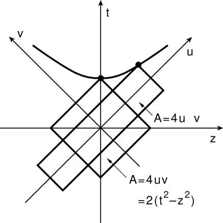
FIG. 1.: Lorentz boost in the light-cone coordinate system.

II Can harmonic oscillators be made covariant?

Quantum field theory has been quite successful in terms of perturbation techniques in quantum electrodynamics. However, this formalism is based on the S matrix for scattering problems and useful only for physical processes where a set of free particles becomes another set of free particles after interaction. Quantum field theory does not address the question of localized probability distributions and their covariance under Lorentz transformations. The Schrödinger quantum mechanics of the hydrogen atom deals with localized probability distribution. Indeed, the localization condition leads to the discrete energy spectrum. Here, the uncertainty relation is stated in terms of the spatial separation between the proton and the electron. If we believe in Lorentz covariance, there must also be a time-separation between the two constituent particles.

Before 1964 [1], the hydrogen atom was used for illustrating bound states. These days, we use hadrons which are bound states of quarks. Let us use the simplest hadron consisting of two quarks bound together with an attractive force, and consider their space-time positions $x_{a}$ and $x_{b}$, and use the variables

$$X=(x_{a}+x_{b})/2,\qquad x=(x_{a}-x_{b})/2\sqrt{2}.$$ (1)

The four-vector $X$ specifies where the hadron is located in space and time, while the variable $x$ measures the space-time separation between the quarks. According to Einstein, this space-time separation contains a time-like component which actively participates as can be seen from

$$\pmatrix{z^{\prime}\cr t^{\prime}}=\pmatrix{\cosh\eta&\sinh\eta\cr\sinh\eta&\cosh\eta}\pmatrix{z\cr t},$$ (2)

when the hadron is boosted along the $z$ direction. In terms of the light-cone variables defined as [8]

$$u=(z+t)/\sqrt{2},\qquad v=(z-t)/\sqrt{2},$$ (3)

the boost transformation of Eq.(2) takes the form

$$u^{\prime}=e^{\eta}u,\qquad v^{\prime}=e^{-\eta}v.$$ (4)

The $u$ variable becomes expanded while the $v$ variable becomes contracted.

Does this time-separation variable exist when the hadron is at rest? Yes, according to Einstein. In the present form of quantum mechanics, we pretend not to know anything about this variable. Indeed, this variable belongs to Feynman’s rest of the universe. In this report, we shall see the role of this time-separation variable in the decoherence mechanism.

Also in the present form of quantum mechanics, there is an uncertainty relation between the time and energy variables. However, there are no known time-like excitations. Unlike Heisenberg’s uncertainty relation applicable to position and momentum, the time and energy separation variables are c-numbers, and we are not allowed to write down the commutation relation between them. Indeed, the time-energy uncertainty relation is a c-number uncertainty relation [9], as is illustrated in Fig. 2

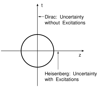
FIG. 2.: Space-time picture of quantum mechanics. There are quantum excitations along the space-like longitudinal direction, but there are no excitations along the time-like direction. The time-energy relation is a c-number uncertainty relation.

How does this space-time asymmetry fit into the world of covariance [10]. This question was studied in depth by the present authors in the past. The answer is that Wigner’s $O(3)$-like little group is not a Lorentz-invariant symmetry, but is a covariant symmetry [3]. It has been shown that the time-energy uncertainty applicable to the time-separation variable fits perfectly into the $O(3)$-like symmetry of massive relativistic particles [4].

The c-number time-energy uncertainty relation allows us to write down a time distribution function without excitations [4]. If we use Gaussian forms for both space and time distributions, we can start with the expression

$$\left({1\over\pi}\right)^{1/2}\exp{\left\{-{1\over 2}\left(z^{2}+t^{2}\right)\right\}}$$ (5)

for the ground-state wave function. What do Feynman et al. say about this oscillator wave function?

In their classic 1971 paper [2], Feynman et al. start with the following Lorentz-invariant differential equation.

$${1\over 2}\left\{x^{2}_{\mu}-{\partial^{2}\over\partial x_{\mu}^{2}}\right\}\psi(x)=\lambda\psi(x).$$ (6)

This partial differential equation has many different solutions depending on the choice of separable variables and boundary conditions. Feynman et al. insist on Lorentz-invariant solutions which are not normalizable. On the other hand, if we insist on normalization, the ground-state wave function takes the form of Eq.(5). It is then possible to construct a representation of the Poincaré group from the solutions of the above differential equation [4]. If the system is boosted, the wave function becomes

$$\psi_{\eta}(z,t)=\left({1\over\pi}\right)^{1/2}\exp\left\{-{1\over 2}\left(e^{-2\eta}u^{2}+e^{2\eta}v^{2}\right)\right\}.$$ (7)

This wave function becomes Eq.(5) if $\eta$ becomes zero. The transition from Eq.(5) to Eq.(7) is a squeeze transformation. The wave function of Eq.(5) is distributed within a circular region in the $uv$ plane, and thus in the $zt$ plane. On the other hand, the wave function of Eq.(7) is distributed in an elliptic region with the light-cone axes as the major and minor axes respectively. If $\eta$ becomes very large, the wave function becomes concentrated along one of the light-cone axes. Indeed, the form given in Eq.(7) is a Lorentz-squeezed wave function. This squeeze mechanism is illustrated in Fig. 3.

There are many different solutions of the Lorentz invariant differential equation of Eq.(6). The solution given in Eq.(7) is not Lorentz invariant but is covariant. It is normalizable in the $t$ variable, as well as in the space-separation variable $z$. How can we extract probability interpretation from this covariant wave function?

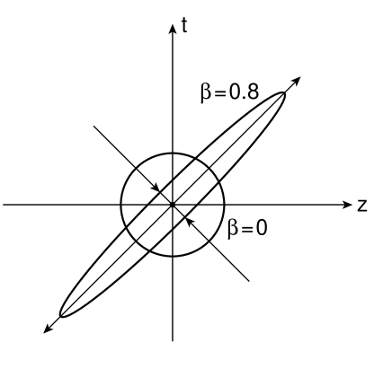
FIG. 3.: Effect of the Lorentz boost on the space-time wave function. The circular space-time distribution at the rest frame becomes Lorentz-squeezed to become an elliptic distribution.

III Probability Interpretation

The wave function of Eq.(7) is a Lorenntz-covariant expression. To an observer in which the hadron is at rest, the parameter $\eta$ becomes zero. For an observer in which the hadron moves very fast, $\eta$ becomes very large. The question then is whether it is possible to construct a probability distribution function from this wave function which contains the time-separation variable $t$.

At this point, it is very important to note that the step toward the construction of the probability distribution not always to take the absolute square of the wave function. The first step is to construct the density matrix which in turn gives the probability distribution. The second step is to sum over or integrate over the variables which are not observed.

Here again let us learn a lesson from Feynman. In his 1972 book on statistical mechanics [5], Feynman says When we solve a quantum-mechanical problem, what we really do is divide the universe into two parts – the system in which we are interested and the rest of the universe. We then usually act as if the system in which we are interested comprised entire universe. To motivate the use of density matrices, let us see what happens when we include the part of the universe outside the system.

It is an interesting exercise to work out a concrete example of Feynman’s rest of the universe. Let us consider two identical coupled oscillators with coordinates $x_{1}$ and $x_{2}$. Here the first coordinate is in the system in which we are interested and the second belongs to the rest of the universe. In order to get the probability distribution in the first coordinate while it is not possible to get any information from the second coordinate, we can construct the density matrix first with both coordinate variables and then integrate over the second variable. The effect of this ignorance is measured in terms of the entropy. This procedure has been discussed in detail in Ref. [11]. Let us outline the content of this paper.

For the coupled harmonic oscillators, the standard procedure is to separate the Hamiltonian using the normal coordinates $\left(x_{1}+x_{2}\right)/\sqrt{2}$ and $\left(x_{1}-x_{2}\right)/\sqrt{2}$. Then the resulting wave function is

$$\psi_{\eta}\left(x_{1},x_{2}\right)=\left({1\over\pi}\right)^{1/2}\exp\left\{-{1\over 4}\left(e^{-2\eta}\left(x_{1}+x_{2}\right)^{2}+e^{2\eta}\left(x_{1}-x_{2}\right)^{2}\right)\right\},$$ (8)

where the parameter $\eta$ in this case measures the strength of coupling. If it is zero, the oscillator system becomes decoupled. Here, it is possible to give probability interpretation in terms of the two normal coordinates as well as in terms of the $x_{1}$ and $x_{1}$ variables.

It is indeed remarkable that the wave function of Eq.(8) is mathematically identical with the covariant oscillator wave function given in Eq.(7). Thus, for the case of the covariant oscillator, we can follow the same logic as in the coupled oscillators. We can now change the variable $x_{1}$ to $z$, the variable in the system we are interested, and $x_{2}$ to $t$ which belongs to the rest of the universe.

With these ingredients in mind, let us start with the square of the covariant wave function of Eq.(7):

$$\rho_{\eta}(z,t)=\psi_{\eta}(z,t)\left(\psi_{\eta}(z,t)\right)^{*}$$ (9)

This is the density matrix if both the $z$ and $t$ variables are taken into account. Since we do not observe $t$ in the present form of quantum mechanics, we have to integrate the above quantity over the $t$ variable.

$$\rho_{\eta}(z)=\int\rho_{\eta}(z,t)dt.$$ (10)

The evaluation of this integral leads to the probability density:

$$\rho_{eta}(z)=\left({1\over\pi(\cosh 2\eta)}\right)^{1/2}\exp{\left({-z^{2}\over\cosh 2\eta}\right)}.$$ (11)

This is a normalized probability distribution function. If the hadronic speed is zero, this expression reduces to the probability density for the ground-state harmonic oscillator.

The wave function becomes wide-spread as $\eta$ increases, but the normalization is preserved. The Lorentz boost is therefore a probability-preserving transformation.

In Ref. [11] in which the coupled oscillator system is discussed, it was observed that our ignorance over the rest of the universe causes an increase in entropy. The expression of the entropy does not contain the coordinate variables there. Thus it should also be independent of $z$ and $t$ variables. The entropy for this system is

$$S=-Tr(\rho~{}\ln(\rho))$$ (12)

$$=-\int\rho(z)\ln\left(\rho(z)\right)dz.$$ (13)

The evaluation of integral leads to

$$S=\left(\cosh{\eta\over 2}\right)^{2}\ln\left(\cosh{\eta\over 2}\right)^{2}-\left(\sinh{\eta\over 2}\right)^{2}\ln\left(\sinh{\eta\over 2}\right)^{2}.$$ (14)

This form is the same as the entropy for thermally-excited oscillator state. The entropy vanishes when the hadron is at rest with $\eta=0$, and increases linearly in $\eta$ as the hadronic speed becomes large.

We learned in this section how to take care of the time-separation variable when we obtain the probability distribution from the covariant wave function of Eq.(7). We learned also that it is now possible to give a probability interpretation of the density function of Eq.(9) in terms of both the $z$ and $t$ variables, as in the case of $x_{1}$ and $x_{2}$ variables for the coupled oscillator case.

IV Feynman’s Parton Picture

It is a widely accepted view that hadrons are quantum bound states of quarks having localized probability distribution. As in all bound-state cases, this localization condition is responsible for the existence of discrete mass spectra. The most convincing evidence for this bound-state picture is the hadronic mass spectra which are observed in high-energy laboratories [2, 4]. However, this picture of bound states is applicable only to observers in the Lorentz frame in which the hadron is at rest. How would the hadrons appear to observers in other Lorentz frames? To answer this question, we can use the picture of Lorentz-squeezed hadrons discussed in Sec. III.

In 1969, Feynman observed that a fast-moving hadron can be regarded as a collection of many “partons” whose properties not appear to be quite different from those of the quarks [7]. For example, the number of quarks inside a static proton is three, while the number of partons in a rapidly moving proton appears to be infinite. The question then is how the proton looking like a bound state of quarks to one observer can appear different to an observer in a different Lorentz frame? Feynman made the following systematic observations.

• The picture is valid only for hadrons moving with velocity close to that of light.

• The interaction time between the quarks becomes dilated, and partons behave as free independent particles.

• The momentum distribution of partons becomes widespread as the hadron moves fast.

• The number of partons seems to be infinite or much larger than that of quarks.

Because the hadron is believed to be a bound state of two or three quarks, each of the above phenomena appears as a paradox, particularly b) and c) together.

In order to resolve this paradox, let us write down the momentum-energy wave function corresponding to Eq.(7). If the quarks have the four-momenta $p_{a}$ and $p_{b}$, we can construct two independent four-momentum variables [2]

$$P=p_{a}+p_{b},\qquad q=\sqrt{2}(p_{a}-p_{b}),$$ (15)

where $P$ is the total four-momentum and is thus the hadronic four-momentum. $q$ measures the four-momentum separation between the quarks. Their light-cone variables are

$$q_{u}=(q_{0}-q_{z})/\sqrt{2},\qquad q_{v}=(q_{0}+q_{z})/\sqrt{2}.$$ (16)

The resulting momentum-energy wave function is

$$\phi_{\eta}(q_{z},q_{0})=\left({1\over\pi}\right)^{1/2}\exp\left\{-{1\over 2}\left(e^{-2\eta}q_{u}^{2}+e^{2\eta}q_{v}^{2}\right)\right\}.$$ (17)

Because we are using here the harmonic oscillator, the mathematical form of the above momentum-energy wave function is identical to that of the space-time wave function. The Lorentz squeeze properties of these wave functions are also the same. This aspect of the squeeze has been exhaustively discussed in the literature [4, 12, 13].

When the hadron is at rest with $\eta=0$, both wave functions behave like those for the static bound state of quarks. As $\eta$ increases, the wave functions become continuously squeezed until they become concentrated along their respective positive light-cone axes. Let us look at the z-axis projection of the space-time wave function. Indeed, the width of the quark distribution increases as the hadronic speed approaches that of the speed of light. The position of each quark appears widespread to the observer in the laboratory frame, and the quarks appear like free particles.

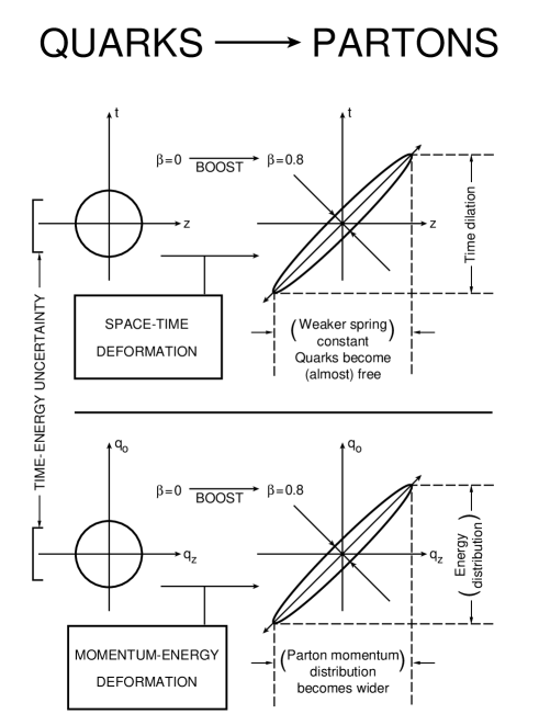
FIG. 4.: Lorentz-squeezed space-time and momentum-energy wave functions. As the hadron’s speed approaches that of light, both wave functions become concentrated along their respective positive light-cone axes. These light-cone concentrations lead to Feynman’s parton picture.

The momentum-energy wave function is just like the space-time wave function, as is shown in Fig. 4. The longitudinal momentum distribution becomes wide-spread as the hadronic speed approaches the velocity of light. This is in contradiction with our expectation from non-relativistic quantum mechanics that the width of the momentum distribution is inversely proportional to that of the position wave function. Our expectation is that if the quarks are free, they must have their sharply defined momenta, not a wide-spread distribution.

However, according to our Lorentz-squeezed space-time and momentum-energy wave functions, the space-time width and the momentum-energy width increase in the same direction as the hadron is boosted. This is of course an effect of Lorentz covariance. This indeed is the key to the resolution of the quark-parton paradox [4, 12].

V Measurement Problem

According to Sec. III, it is possible to define the covariant probability distribution function in terms of both the space and time separation variables. Indeed, the quark distribution can be covariantly transformed according to Fig. 4. In this section, we address the question of how partons interact incoherently with external signals.

When the hadron is boosted, the hadronic matter becomes squeezed and becomes concentrated in the elliptic region along the positive light-cone axis, as is illustrated in Figs. 3 and 4. The length of the major axis becomes expanded by $e^{\eta}$, and the minor axis is contracted by $e^{-\eta}$.

This means that the interaction time of the quarks among themselves becomes dilated. Because the wave function becomes wide-spread, the distance between one end of the harmonic oscillator well and the other end increases. This effect, first noted by Feynman [7], is universally observed in high-energy hadronic experiments. The period of the oscillation increases like $e^{\eta}$.

On the other hand, the interaction time with the external signal, since it is moving in the direction opposite to the direction of the hadron, travels along the negative light-cone axis. If the hadron contracts along the negative light-cone axis, the interaction time decreases by $e^{-\eta}$. The ratio of the interaction time to the oscillator period becomes $e^{-2\eta}$. The energy of each proton coming out of the Fermilab accelerator is $900GeV$. This leads the ratio to $10^{-6}$. This is indeed a small number. The external signal is not able to sense the interaction of the quarks among themselves inside the hadron.

Indeed, Feynman’s parton picture is one concrete physical example where the decoherence effect is observed. As for the entropy, the time-separation variable belongs to the rest of the universe. Because we are not able to observe this variable, the entropy increases as the hadron is boosted to exhibit the parton effect. The decoherence is thus accompanied by an entropy increase.

Let us go back to the coupled-oscillator system. The light-cone variables in Eq.(7) correspond to the normal coordinates in the coupled-oscillator system given in Eq.(LABEL:normal). According to Feynman’s parton picture, the decoherence mechanism is determined by the ratio of widths of the wave function along the two normal coordinates, or along the two light-cone coordinates. Indeed, Feynman’s decoherence is observed in the light-cone coordinate system.

Concluding Remarks

The present authors have been interested in question of covariant probability distribution since 1973 [10]. We started with the covariant oscillator wave function as a purely phenomenological mathematical instrument. We then noticed that the covariant oscillator formalism can serve as a representation of the Wigner’s little group for massive particles, capable of the fundamental symmetry representation for relativistic particles. This allows us to deal with the c-number time-energy uncertainty relation without excitations.

Later, we were able to illustrate Feynman’s rest of the universe in terms of two coupled oscillators. By comparing the covariant oscillator with the coupled oscillator, we are able to give a covariant probability interpretation to the density matrix depending on both the space-separation and time-separation variables.

This covariant probability distribution function can provide a resolution to the quark-parton puzzle which includes Feynman’s decoherence.

REFERENCES

- [1] M. Gell-Mann, Phys. Lett. 13, 598 (1964).
- [2] R. P. Feynman, M. Kislinger, and F. Ravndal, Phys. Rev. D 3, 2706 (1971).
- [3] E. P. Wigner, Ann. Math. 40, 149 (1939).
- [4] Y. S. Kim and M. E. Noz, Theory and Applications of the Poincaré Group (Reidel, Dordrecht, 1986).
- [5] R. P. Feynman, Statistical Mechanics (Benjamin/Cummings, Reading, MA, 1972).
- [6] J. von Neumann, Die mathematische Grundlagen der Quanten-mechanik (Springer, Berlin, 1932). See also J. von Neumann, Mathematical Foundation of Quantum Mechanics (Princeton University, Princeton, 1955).
- [7] R. P. Feynman, The Behavior of Hadron Collisions at Extreme Energies, in High Energy Collisions, Proceedings of the Third International Conference, Stony Brook, New York, edited by C. N. Yang et al., Pages 237-249 (Gordon and Breach, New York, 1969).
- [8] P. A. M. Dirac, Rev. Mod. Phys. 21, 392 (1949).
- [9] P. A. M. Dirac, Proc. Roy. Soc. (London) A114, 234 and 710 (1927).
- [10] Y. S. Kim and M. E. Noz, Phys. Rev. D 8, 3521 (1973).
- [11] D. Han, Y. S. Kim, and M. E. Noz, Am. J. Phys. 67, 61 (1999).
- [12] Y. S. Kim and M. E. Noz, Phys. Rev. D 15, 335 (1977).
- [13] Y. S. Kim, Phys. Rev. Lett. 63, 348 (1989).