Quantum state tomography of dissociating molecules

Abstract

Using tomographic reconstruction we determine the complete internuclear quantum state, represented by the Wigner function, of a dissociating I₂ molecule based on femtosecond time resolved position and momentum distributions of the atomic fragments. The experimental data are recorded by timed ionization of the photofragments with an intense 20 fs laser pulse. Our reconstruction method, which relies on Jaynes’ maximum entropy principle, will also be applicable to time resolved position or momentum data obtained with other experimental techniques.

Quantum state tomography derives its name from the tomographic technique in medical diagnostics by which three-dimensional images of the inner parts of an object or a person can be derived from two-dimensional NMR or X-ray pictures obtained from different directions, a technique for which Cormack and Hounsfield were awarded the Nobel prize in physiology and medicine in 1979. In quantum physics, we often deal with a phase space, characterizing the position and velocity distribution of particles, and the aim of quantum state tomography is to determine this distribution from only position and momentum measurements on the particles. As an example, the oscillatory motion of a particle in a quadratic potential is described as a simple rotation in phase space, and hence the mathematical Radon-transform technique Natterer , used in physiology and medicine can be used to extract the phase space distribution of such a particle if only position measurements are made sufficiently often over a time corresponding to the oscillation period. This technique has been succesfully applied to analyze bound molecular states, where the internuclear distance oscillates harmonically Whamsley , and it has been used for non-classical states of light Raymer ; Mlynek , which are formally described as harmonically trapped particles. A number of extensions have been made to incorporate anharmonicities in the trapping potential, and to use mathematical reconstruction techniques which match specific detection schemes Leonhardt ; Vogel ; Wineland ; Haroche . In the present work we determine the internuclear quantum state of dissociating $I_{2}$ molecules. The atomic fragments are created in a state with positive energy, and they fly apart with no confining force between them. The situation thus differs from the one of trapped motion, and it calls for a new theoretical approach.

Experimentally, $I_{2}$ molecules in a molecular beam are photodissociated by irradiation with a 100-fs-long pump pulse centered at 488 nm (see Fig. 1). To determine the internuclear separation (position) and velocitiy (momentum) of the dissociating molecules at time $\tau$ after excitation the atomic $I$ fragments are ionized by a 20-fs-long probe pulse, and the velocities of the $I^{+}$ ions are measured by a 2-dimensional ion detector skovsen . If only one of the iodine atoms of a dissociating molecule is ionized the $I^{+}$ velocity is equal to half of the internuclear velocity, approximately 4.0 Å/ps. On the 2-D image, shown in Fig. 1, these ions constitute the innermost pair of half rings ($I^{+}$-$I$). If, instead, both iodine atoms are ionized the velocity of the $I^{+}$ ions is increased due to their internal Coulomb repulsion. On the 2-D image these ions constitute the outermost pair of half rings ($I^{+}$-$I^{+}$). Using Coulomb’s law the $I^{+}$ velocity distribution from this channel gives directly the internuclear distribution skovsen .

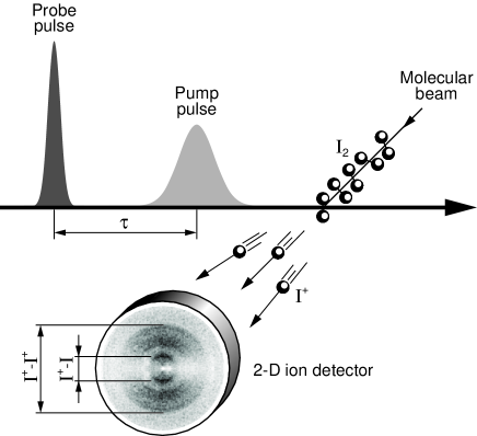
Figure 1: Diagram of the experimental setup showing the molecular beam crossed at 90^o by the pump and the probe laser beams. Both laser beams are polarized vertically. The $I^{+}$ ions produced are pushed by a weak electrostatic field (not shown) towards a 2-D ion detector, where their positions are used to determine the internuclear velocity distribution ($I^{+}$-$I$ channel) and the internuclear separation distribution ($I^{+}$-$I^{+}$ channel). The image shown on the detector is recorded for a delay of 5 ps between the pump and the probe pulse.

The atomic density is sampled on a discrete position grid with $N$ grid points, where $N=51$ in the example shown in Fig. 2. For the data presented here, the reconstruction is based on position distributions recorded at $\tau$ = 2, 3, 4, 5 picoseconds (ps) and the momentum distribution (which is identical at the four different delays). In quantum tomography on harmonic oscillator states the fast and slow velocity components are slushing back and forth, and the time dependent position distribution maps the phase space distribution from all angles. In free expansion, slow particles will not be able to catch up on fast ones, and we have access to only sheared pictures of the distribution where the high velocity components are shifted towards larger displacements than the low velocity components. This implies that a range of angular viewing angles is missing, and we cannot apply the Radon transform to reconstruct the phase space distribution.

Furthermore, the data-sets are noisy due to the finite counts in different position intervals, and our task is to establish the most reliable estimate of $\rho$ in best possible (rather than perfect) agreement with the observed data. Following Drobny and Buzek Drobny , we apply Jaynes’ maximum entropy principle which at the same time provides the smallest deviation from the measured data and the largest possible von Neumann entropy Drobny ; Jaynes : $S(\rho)=-Tr(\rho\ln\rho)$. Drobny and Buzek have used the maximum entropy principle for quantum state tomography on harmonically trapped atoms detected at too few instants of time to allow a normal reconstruction Drobnyatom , and we have reformulated their method to deal with free atoms.

To calculate the von Neumann entropy, one may use the familiar expression in terms of the eigenvalues $p_{j}$ of the density matrix, $S=-\sum_{j}p_{j}\ln p_{j}$, but as it was shown by Jaynes Jaynes , it is not necessary to compute the entropy of $\rho$ in order to use the maximum entropy principle: The density matrix with largest entropy which conforms best with measured values $a_{i}$ for a set of observables $A_{i}$, can be written on the form

$$\rho=\frac{1}{Z}\exp(-\sum_{i}\lambda_{i}A_{i}),$$ (1)

where $\lambda_{i}$ are variables that have to be adjusted to satisfy the agreement with the measured data, and $Z$ normalizes the density matrix to unit trace.

A position distribution is the set of expectation values of projection operators on position eigenstates $|x\rangle\langle x|$. We determine the position distribution at different times, and we need a formal representation of the projection operator $|x,t\rangle\langle x,t|$ where $|x,t\rangle$ is a position eigenstate at time $t$. For free particles the momentum $p=\hbar k$ is a conserved quantity, and it is convenient to represent the projection operators in a momentum representation, since momentum eigenstates accumulate only a trivial phase factor with time, $|k,t\rangle=\exp(i\hbar k^{2}t/2M)|k,t=0\rangle$:

$$|x\rangle\langle x|=\int dk_{1}dk_{2}|k_{1}\rangle\langle k_{1}|x\rangle\langle x|k_{2}\rangle\langle k_{2}|$$

$$=\frac{1}{2\pi}\int dk_{1}dk_{2}\exp(i(k_{2}-k_{1})x)|k_{1}\rangle\langle k_{2}|.$$ (2)

Both the spatial distribution at various times and the momentum distribution, which is independent of time, are measured, and the observables $A_{i}$ in Eq.(1) are precisely the operators $|x,t\rangle\langle x,t|$ and $|k\rangle\langle k|$, which are now given explicity as $N$ by $N$ matrices in a discrete basis. The exponential in Eq.(1) is understood as a matrix power series, and it has to be evaluated numerically because the momentum projection operators and the position projection operators at different times do not commute.

In our numerical reconstruction we used four position distributions and one momentum distributions, and we thus identified $5\cdot 51$ variables $\lambda_{i}$ so that the expectation values $\langle A_{i}\rangle=$Tr$(\rho A_{i})$ are as close as possible to the measured distributions. We quantify the agreement with the measured data $a_{i}$ by the sum of the squares of all deviations $\Delta=\sum_{i}(a_{i}-\langle A_{i}\rangle)^{2}$. A numerical routine identifies the global minimum of $\Delta$ as a function of the $\lambda_{i}$ variables, and we thus obtain the explicit expression for the density matrix in Eq.(1).

To illustrate our reconstruction of the internuclear quantum state of the dissociated molecules we use the Wigner function $W(x,p)$ Hillery rather than the N by N complex density matrix, discussed above. The Wigner function is obtained by a Fourier transform with respect to the difference between the two momentum arguments in the density matrix. While still fully characterizing the quantum state the Wigner function is a real function, and it has the advantage of presenting at one glance the joint position and momentum distribution. Figure 2 shows the Wigner function, $W(x,p)$, at the earliest (2 ps) and the latest time (5 ps) for which position distributions were recorded. Note that we present the momentum dependence in units of the velocity $v=p/M$ of the atomic fragments to facilitate comparison of the two panels. The two Wigner functions in Fig. 2 a) and b) have the same velocity distributions, but they are sheared differently in phase space due to the free motion of the two iodine photofragments. On the side panels the marginal position and velocity distribution, obtained by integrating $W(x,p)$ over velocity and position, respectively, are compared with the experimental results (open circles). The agreement is excellent, and similar good agreement is found between the measured data and the reconstructed state at the intermediate times at 3 and 4 ps.

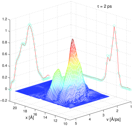
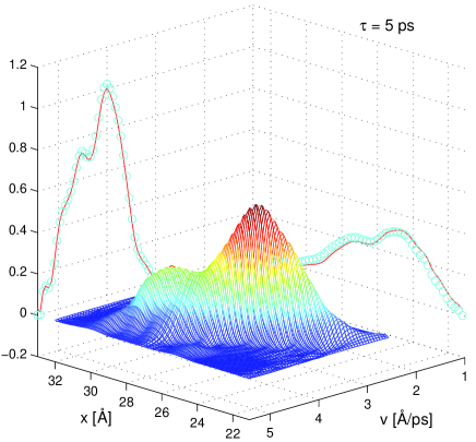
Figure 2: Three dimensional surface plots showing the phase space distribution function $W(x,p)$ (Wigner function) at two different times after the pump pulse dissociates the $I_{2}$ molecule (tau=2ps in part (A) and tau = 5 ps in part (B)). The marginal position and momentum distributions of the dissociated molecules are shown on the side panels: The full curves are the reconstructed distributions (integrals over the Wigner function with respect to momentum and position, respectively), and the open circles are the measured distributions. To provide a more intuitive view the momentum variable is presented in velocity units.

We stress that the Wigner function contains more information than what can be obtained directly from a single measured position and velocity distribution. For instance, both the measured position and velocity distribution at 2 ps consists of two peaks (side panels of Fig. 2 (A)), but without further information it is not possible to determine if the molecules at the larger internuclear separation (the peak around 13.6 Å ) are also the ones moving with the largest internuclear velocity (the peak around 4.6 Å/ps). The tomographic reconstruction of the Wigner function makes use of our knowledge of the position distributions measured at 3, 4 and 5 ps, and, indeed, the two separated peaks in $W(x,p)$ at 2 ps show that the iodine atoms roughly 13.6 Å apart have a velocity distribution centered around 4.6 Å/ps whereas the iodine atoms apparoximately 12.4 Å apart have a velocity distribution centered at 4.0 Å/ps. The physical origin of the two internuclear velocity components is the incoherent population of v = 0 and v = 1 vibrational levels of the electronic ground state of the I₂ molecules prior to dissociation by the pump pulse skovsen .

It has been emphasized in the literature Hillery that the Wigner function is not a real probability distribution because, due to complimentarity and Heisenbergs’s uncertainty relation, it is not meaningful to assign precise values for both the position and velocity of a particle. This has as its most striking consequence that states exist for which $W(x,p)$ attains negative values, but these negative values always occur in phase space regions with area less than Planck’s constant $\hbar=h/2\pi$. Dissociation of molecules by two phase-locked femtosecond laser pulses will produce photofragments in a coherent superposition of two localized wave packets skovsen , and we are currently working on improvement of the experiments to enable reconstruction of the Wigner function with a sufficient resolution to display the negativities expected in this case. Such an experiment constitutes a fs time resolved analogue to double-slit atom interferometer studies Mlyneknature .

Quantum state tomography has been established in quantum optics as a remarkable diagnostics tool that has provided clear illustrations of the experimental ability to control and manipulate selected states of fundamental quantum systems such as a single field mode and single ions and atoms Mlynek ; Vogel ; Drobnyatom ; Wineland ; Haroche . Our experimentally reconstructed density matrix or Wigner function provides the complete information about the non-trivial quantum state of the internuclear motion of the dissociating $I_{2}$ molecules. Although our experimental method is limited to small molecules, we believe that quantum state tomography will be applicable also to study chemical reactions in large molecules through time resolved position data obtained, e.g., by the emerging femtosecond electron and X-ray diffraction techniques Ihee ; Reutze ; Corkum ; Service . This will open for comparisons with theoretical calculations at a much more detailed level than probability distributions of single observables, which have formed the basis of comparison so far in femtosecond time resolved chemical reaction dynamics. Finally, we note that modern femtosecond laser technology enables controlled shaping of both the electronic and the atomic structure of molecules through irradiation with sequences of tailored laser pulses Rabitz ; Levis ; Gerber . To fully exploit the capabilities of such quantum manipulation it is crucial to completely characterize the molecular quantum states formed.

We acknowledge the support from the Carlsberg Foundation and The Danish Natural Science Council.

References

- (1) F. Natterer, The Mathematics of Computerized Tomography (Wiley, New York, 1986).
- (2) T. J. Dunn, I. A. Walmsley, and S. Mukamel, Phys. Rev. Lett. 74, 884-887 (1995).
- (3) D. T. Smithey, M. Beck, and M. G. Raymer, Phys. Rev. Lett. 70, 1244-1247 (1993).
- (4) A. I. Lvovsky, et al, Phys. Rev. Lett. 87, 050402 (2001).
- (5) U. Leonhardt, Phys. Rev. A, 53 2998-3013 (1996).
- (6) S. Wallentowitz, and W. Vogel, Phys. Rev. Lett. 75, 2932-2935 (1995).
- (7) D. Leibfried, et al, Phys. Rev. Lett. 77, 4281-4285 (1996).
- (8) P. Bertet, P. et al., Phys. Rev. Lett. 89, 200402 (2002).
- (9) E. Skovsen, M. Machholm, T. Ejdrup, J. Thgersen, and H. Stapelfeldt, Phys. Rev. Lett. 89, 133004 (2002).
- (10) V. Buzek, and G. Drobny, J. Mod. Opt. 47, 2823-2839 (2000).
- (11) E. T. Jaynes, Phys. Rev. 106, 620-630; 108, 171 (1957).
- (12) G. Drobny, and V. Buzek, Phys. Rev. A 65, 053410 (2002).
- (13) M. Hillery, R. F. O’Connell, M. O. Scully, and E. P. Wigner, Phys. Rep. 106, 121-167 (1984).
- (14) Ch. Kurtsiefer, T. Pfau, and J. Mlynek, Nature 386, 150-153 (1997).
- (15) H. Rabitz, R. de Vivie-Riedle, M. Motzkus and K. Kompa, Science 288, 824-828 (2001).
- (16) R. J. Levis, G. M. Menkir, H. Rabitz, Science 292, 709-713 (2001).
- (17) T. Brixner, N. H. Damrauer, P. Nikalus, and G. Gerber, Nature 414, 57-60 (2001).
- (18) Ihee, H. et al. Science 291, 458-462 (2001).
- (19) R. Neutze, R. Wouts, D. van der Spoel, E. Weckert, and J. Hajdu, Nature 406, 752-757 (2000).
- (20) H. Niikura et al, Nature 417, 917-922 (2002).
- (21) R. F. Service, Science 298, 1356-1358 (2002).