Propagation, breathing and transition of matter-wave packet trains

Abstract

We find a set of new exact solutions of a quantum harmonic oscillator, which describes some wave-packet trains with average energy being proportional to both the quantum level and classical energy of the oscillator. Center of the wave-packet trains may oscillate like a classical harmonic oscillator of frequency $\omega$. Width and highness of the trains may change simultaneously with frequency $2\omega$ as an array of breathers. Under some perturbations the wave-packet trains could transit between the states of different quantum numbers. We demonstrate analytically and numerically that the wave-packet trains can be strictly fitted to the matter-wave soliton trains observed by Strecher et al. and reported in Nature 417, 150(2002). When the wave-packets breathe with greater amplitudes, they show periodic collapse and revival of the matter-wave.

PACS numbers: 03.75.-b, 03.65.Ge, 05.30.Jp

As an elementary equation of quantum mechanics the Schr$\ddot{o}$dinger equation is a linearly partial differential one of the second order with variable coefficients [1]-[3]. We well known that this equation cannot be exactly solved yet for most physically interesting systems, except a few systems with separation of variables such as hydrogen atom, harmonic oscillator and rigid rotator [4], [5]. The quantum states described by its solutions with inseparable space-time variables are very important but difficult to find. The coherent state of a harmonic oscillator is a nice example of such states [6]-[8]. To seek new inseparable exact solutions of a Schr$\ddot{o}$dinger equation and to physically realize them are our main motivations in this paper.

The preparation and measurement of quantum states are very hard even impossible for some microscopic systems [9]- [11]. Compared to this the physical realization and detection of the macroscopic and mesoscopic quantum states may be easier sometimes [12], [13]. The Bose-Einstein condensate (BEC) just supplies such a macroscopic quantum system [14]-[16], which can be use to test the Schr$\ddot{o}$dinger quantum mechanics. For example, a harmonically confined BEC can be identified as a perturbed quantum harmonic oscillator, when the interatomic interaction is weak enough [17], [18]. The weak atom-atom interactions were due to the small atomic samples [19], [20] and short $s$-wave scattering length $|a|$ [21], [22] that can be controlled by the Feshbach resonance [23], [24].

A quite interesting phenomenon was experimentally observed that the weakly interacting BEC appears solitonlike behavior [21], [22]. Although this was approximately explained by using nonlinear interaction [25], [26], Strecher and coworkers said that ”non-interacting solitons $\cdots$ would be expected to pass through one another” in their experiment. The solitonlike behavior is also explored for ideal BEC gas with $a=0$ in Khaykovich’s experiment. Another important fact is the finding of collapse and revival of the macroscopic matter-wave packets [27], [28], which can occur for very weak interaction with atomic samples composed of a few thousand particles [19]. In this paper we shall report a set of new exact solutions of a quantum harmonic oscillator and the corresponding macroscopic quantum level. By using them we demonstrate that, analytically and numerically, the wave-packet trains governed by these exact solutions can be strictly fitted to the matter-wave soliton trains found by Strecher et al.. This result means that Strecher’s ”non-interacting solitons” had been observed by themselves. On the other hand, under some particular initial and boundary conditions, these solutions exactly describe the well-known collapse and revival of a weakly interacting BEC.

We consider a BEC consisting of $N$ identical Bose atoms and being transferred into a cigar-shaped magneto-optical trap. Dynamics of the system is governed by the Gross-Pitaevskii equation (GPE) [17], [18]

$$i\hbar\frac{\partial\psi}{\partial t}=-\frac{\hbar^{2}}{2m}\bigtriangledown^{2}\psi+\Big{[}\frac{1}{2}m\omega_{x}^{2}x^{2}+\frac{1}{2}m\omega_{r}^{2}(y^{2}+z^{2})+g_{0}|\psi|^{2}\Big{]}\psi,$$ (1)

where $\omega_{r}$ and $\omega_{x}$ are the transverse and axial frequencies respectively, the interaction intensity $g_{0}$ is related to the $s$-wave scattering length $a$, atomic mass $m$ and number of atoms $N$ through $g_{0}=4\pi N\hbar^{2}a/m$ for the normalized wave-function $\psi$. The norm $|\psi|^{2}$ is the probability density and $N|\psi|^{2}$ the density of atomic number. Setting $l_{r}=\sqrt{\hbar/(m\omega_{r})},\ l_{x}=\sqrt{\hbar/(m\omega_{x})}$ and writing $E_{kin}$ and $E_{int}$ as the kinetic energy and mean-field interaction energy of the BEC, the relationship $E_{int}/E_{kin}\sim N|a|/(l_{r}^{2}l_{x})^{1/3}$ expresses the importance of the atom-atom interaction compared to the kinetic energy [17]. For low particle number [19], [20] or short $s$-wave scattering length $|a|$ [21], [22], we can treat the interaction term as a perturbation [19] and obtain the leading order solution of Eq. (1) to obey the linear Schr$\ddot{o}$dinger equation of a harmonic oscillator. Assuming the leading order wave-function is in the form of separation variable $\Psi_{n}=\psi_{n}(x,t)\psi_{y}(y)\psi_{z}(z)$ and its transverse factor is in the ground state of harmonic oscillator, we find a new exact solution of the linear Schr$\ddot{o}$dinger equation (see Appendix A)

$$\Psi_{n} = \psi_{n}(x,t)\psi_{y}(y)\psi_{z}(z)=R_{n}(x,y,z,t)\exp[i\Theta_{n}(x,t)],$$

$$R_{n} = \Big{[}\frac{\sqrt{c_{0}}}{\pi\sqrt{\pi}l_{r}^{2}l_{x}2^{n}n!\rho(t)}\Big{]}^{1/2}H_{n}(\xi)\exp\Big{[}-\frac{1}{2}\Big{(}\frac{y^{2}}{l_{r}^{2}}+\frac{z^{2}}{l_{r}^{2}}+\xi^{2}\Big{)}\Big{]},\ \ \xi=\frac{\sqrt{c_{0}}x}{\rho(t)l_{x}}-\frac{b_{0}}{\sqrt{c_{0}}}\cos\theta(t),\ \ \$$ (2)

$$\Theta_{n} = \frac{\dot{\rho}(t)x^{2}}{2\rho(t)l_{x}^{2}}-\frac{b_{0}x}{\rho(t)l_{x}}\sin\theta(t)+\frac{b_{0}^{2}}{4c_{0}}\sin[2\theta(t)]-\Big{(}\frac{1}{2}+n\Big{)}\theta(t)-\omega_{r}t,\ \ n=0,\ 1,\ 2,\cdots.$$

Here $b_{0}$ is an arbitrary constant, $H_{n}(\xi)$ denotes the Hermitian polynomial of variable $\xi,\ c_{0}=\dot{\theta}(t)\rho^{2}(t)=AB\omega_{x}\sin(\alpha-\beta)$ is a conserved quantity of the classical harmonic oscillator equation $\ddot{\varphi}=-\omega_{x}^{2}\varphi$ with the complex solution $\varphi=\rho(t)\exp[i\theta(t)],\ \rho(t)$ and $\theta(t)$ are the amplitude and phase of the complex oscillator

$$\rho=\sqrt{A^{2}\cos^{2}(\omega_{x}t+\alpha)+B^{2}\cos^{2}(\omega_{x}t+\beta)},\ \ \theta=\arctan\frac{B\cos(\omega_{x}t+\beta)}{A\cos(\omega_{x}t+\alpha)}$$ (3)

with $A,\ B,\ \alpha$ and $\beta$ being arbitrary constants adjusted by the initial conditions of the classical harmonic oscillator. Obviously, the exact solution is not a energy eigenstate, but denotes a new kind of coherent states. In mathematical point of view, it is a complete solution with independent constants $A,\ B,\ \alpha,\ \beta$ and $b_{0}$. By adjusting these constants, we can use the exact solution to describe some different experimental results. It is easily to prove the exact solution (2) obeying the orthonormalization condition (see Appendix A).

Amplitude $R_{n}$ of the exact solution (2) describes the wave-packet trains consisting of $n+1$ packets. By using Eq. (3), from $\xi=0$ we have orbit of the center of wave-packet trains

$$x_{c}=\frac{b_{0}}{c_{0}}\rho(t)\cos\theta(t)=\frac{b_{0}}{c_{0}}A\cos(\omega_{x}t+\alpha),$$ (4)

which is proportional to real part of the complex solution $\varphi$ for a classical harmonic oscillator of unit mass with amplitude $Ab_{0}/c_{0}$, frequency $\omega_{x}$ and initial phase $\alpha$. We call average energy of the system in state (2) as the macroscopic quantum level, which reads (see Appendix B)

$$E_{n}=\Big{(}\frac{1}{2}+n\Big{)}\frac{c_{1}}{c_{0}}+\omega_{r}+\frac{b_{0}^{2}}{c_{0}}c_{2},\ \ \ \ n=0,\ 1,\ 2,\ \cdots,$$ (5)

where constant $c_{1}=(\dot{\rho}^{2}+c_{0}^{2}/\rho^{2}+\rho^{2}\omega_{x}^{2})/2$ is another conserved quantity of the classical complex oscillator (3), $b_{0}^{2}c_{2}/c_{0}=b_{0}^{2}A^{2}c_{1}/[c_{0}^{2}(A^{2}+B^{2})]$ is proportional to square of the amplitude of Eq. (4) or energy of the classical oscillator. Here and the following, we adopt the natural unit with $m=\hbar=\omega_{x}=1$ such that $\omega_{r}$ is normalized by $\omega_{x}$. For given constants, Eq. (5) exhibits that the energy only depends on the quantum number $n$. It is quite interesting that the average energy (5) is proportional to both the quantum level and the classical energies of the harmonic oscillators governed by Eqs. (3) and (4).

The function $\rho(t)$ included in $\xi$ describes not only the total width of a wave-packet train but also the width of each packet. The average width of the packets is $\rho(t)/\sqrt{c_{0}}$. Same function in radical of Eq. (2) governs highnesses of every packets. These and Eq. (3) infer that the widths and highnesses may change simultaneously with frequency $2\omega$. When the changes of the widths and highnesses are small, behavior of the wave-packet trains seemingly to be an array of solitons. And larger changes of the widths and highnesses show collapse and revival of the wave-packet trains, like multiple breathers. The normalization condition implies that the broader wave-packet train is associated with smaller mean highness and the narrower wave-packet train corresponds to larger mean highness. In the process of propagation and breathing, the wave-packet trains may spontaneously transit from state of higher average energy to that of lower one. Some perturbations also could cause transition between the states of different quantum numbers. All of these will be numerically illustrated as follows.

Propagation of the wave-packet trains: pure bright soliton trains A pure soliton always keeps its shape and energy in propagation, which can be described by the exact solution (2) through selecting $\rho$ as a constant to fix the width and highness of each wave-packet. To do this we only require limiting the constants in Eq. (3) to $A=B$ and $\beta=\alpha-\pi/2$ such that $\rho=A$. Adopting such selection to the second of Eq. (3) and to the formulas of constants $c_{i}$ leads to the function $\theta(t)=\omega_{x}t+\alpha$ and constants $c_{0}=A^{2}\omega_{x},\ c_{1}=\omega_{x}^{2}A^{2},\ c_{2}=\omega_{x}/2$. In this case the ground state of Eq. (2) with $n=0$ is just the common coherent state of a harmonic oscillator [6]-[8]. Inserting these constants into Eq. (5) yields the average energy $E_{n}=(1/2+n)\omega_{x}+\omega_{r}+b_{0}^{2}/(2A^{2})$. Final term of the energy is just the energy of classical harmonic oscillator (4), namely $\frac{1}{2}\omega_{x}^{2}(b_{0}A/c_{0})^{2}=b_{0}^{2}/(2A^{2})$. Therefore, the average energy equates to sum of the quantum level and classical energy. We take the parameter set $n=10,\ \alpha=0,\ \beta=-\pi/2,\ A=B=\rho=c_{0}=1,\ b_{0}=-5,\ \omega_{r}=40\omega_{x}$ and adopt the units of time, space and probability density as $\omega_{x}^{-1},\ l_{x}$ and $l_{x}^{-3}$ from Eq. (2) to make the plot of $R^{2}$ on $xoy$ plane for different times. In 1-3 lines of Fig. 1, we show the motions of eleven pure solitons from $t=0,\ x_{c}(0)=-5l_{x}$ to $\omega_{x}t=\pi/2,\ x_{c}(\pi/2)=0$, and to $\omega_{x}t=\pi,\ x_{c}(\pi)=5l_{x}$. In the propagation, the soliton train keeps its shape and distance between two solitons.

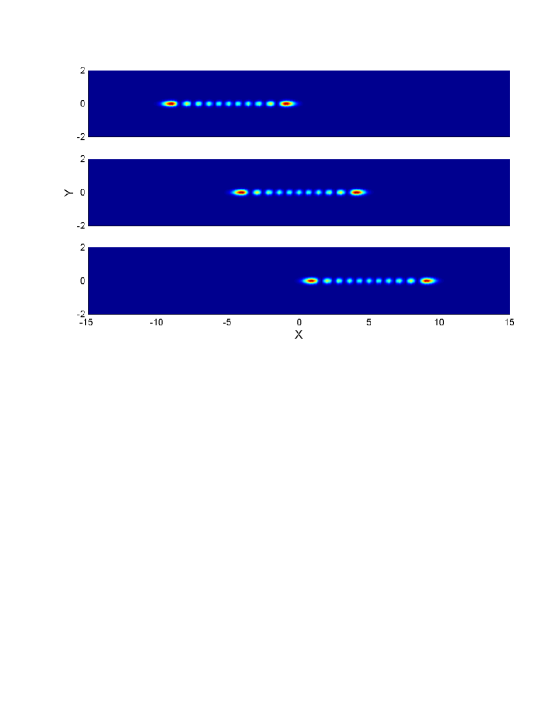
Figure 1: The probability density of the wave-packet train as pure multi-solitons. Taking the parameter set $n=10,\ \alpha=0,\ \beta=-\pi/2,\ A=B=\rho=c_{0}=1,\ b_{0}=-5,\ \omega_{r}=40\omega_{x}$ and normalizing the time, space and probability density in units $\omega_{x}^{-1},\ l_{x}$ and $l_{x}^{-3}$, from Eq. (2) we make the plot of $R^{2}$ on $xoy$ plane for different times. In the first line of Fig. 1 the initial profile of the soliton train is exhibited on left side of the trap. The soliton train propagates to center of the trap at $\omega_{x}t=\pi/2$ and to right side of the trap at $\omega_{x}t=\pi$, as in the second and third lines of Fig. 1.

Breathing of the wave-packet trains: collapse and revival For a very small constant $b_{0}$, Eq. (4) indicates that the amplitude of wave-packet oscillation may be very small. When the constant $b_{0}$ is taken as zero, center of the wave-packet trains is fixed to $x_{c}=0$ and their energy is reduce to $E_{n}=\Big{(}\frac{1}{2}+n\Big{)}\frac{c_{1}}{c_{0}}+\omega_{r}$ by Eq. (5). In order to show the collapse and revival, we let constant $B$ be much greater than $A$, namely $B=1$ and $A=0.01$ such that the highness and width of the wave-packet trains oscillate with greater amplitudes. The other parameters are taken as $n=10,\ \alpha=0,\ \beta=-\pi/2,c_{0}=AB=0.01,\ \omega_{r}/\omega_{x}=l_{x}^{2}/l_{r}^{2}=40$. Using the units of space-time coordinates and probability density of Fig. 1, we numerically draw the plots of vertical view for the wave-packet trains as Fig. 2.

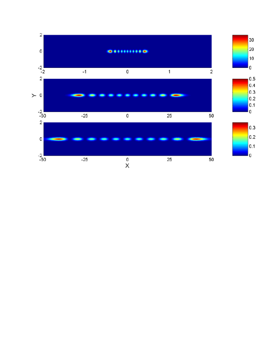
Figure 2: Collapse and revival of the wave-packet trains described by Eqs. (2) and (3) with parameters $n=10,\ b_{0}=0,\ A=c_{0}=0.01,\ B=1,\ \alpha=0,\ \beta=-\pi/2,\ \omega_{r}/\omega_{x}=l_{x}^{2}/l_{r}^{2}=40$. The space-time coordinates and the density are normalized in same units with Fig. 1. Different colors represent different highnesses of the wave-packets as in right side of each line of Fig. 2. The initially high and narrow wave-packet train is shown in the first line of Fig. 2. As time increases to $\omega_{x}t=\pi/4$, the wave-packets collapse to highness of $10^{-1}$ order, as in the second line of Fig. 2. To the half period $\omega_{x}t=\pi/2$, the highness is reduced to $10^{-2}$ order, as in final line of Fig. 2.

In Fig. 2 we exhibit that center of the wave-packet train is fixed at $x_{c}=0$, width and highness of each packet are greatly changed with period $\pi$. The first line of Fig. 2 is corresponded to the initial wave-packet train, which is higher and narrower. The second line of Fig. 2 shows the highnesses of packets have been reduced to $10^{-1}$ order at $\omega_{x}t=\pi/4$, and total width of the wave-packet train is simultaneously raised to $38(l_{x})$. The highness and width of the wave-packet train are collapsed to $10^{-2}$ order and $45(l_{x})$ respectively, when time equates to the half period, as in third line of Fig. 2. In the next half period, revival of the wave-packet train will occur, through an inverse process of that described by Fig. 2. Fixing constant $B$, the forms of Eqs. (2) and (3) means that highnesses of the wave-packets are inversely proportional to constant $A$. When this constant is taken as very small, $A\approx 0$, highness of the wave-packet near $x=0$ will tend to infinity, resulting in the intermittent implosions of the BEC [29], [30].

Strecher’s matter-wave soliton trains Generally, the wave-packet trains governed by Eq. (2) will propagate and breathe simultaneously, and spontaneously transit sometimes. We shall demonstrate that these behaviors can be strictly fit to Strecher’s matter-wave soliton trains. In the experiment reported by Strecher and coworkers [21], the ⁷Li atomic BEC is employed to create the soliton trains, by using a Feshbach resonance to manipulate the sign and magnitude of the $s$-wave scattering length $a$. For a small value of $|a|$ and treating the atom-atom interaction as a perturbation proportional to $a$, the non-interacting soliton trains may be generated.

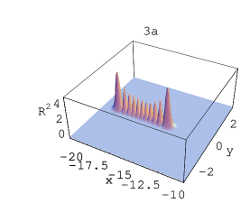
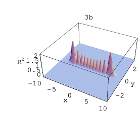
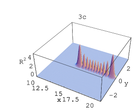
Figure 3: The Strecher’s matter-wave soliton trains on $xoy$ plane from Eqs. (2) and (3) with the parameters $n=10,\ A=c_{0}=0.4624,\ B=1,\ \alpha=0,\ \beta=-\pi/2,\ b_{0}=-17.437,\ \omega_{r}/\omega_{x}=l_{x}^{2}/l_{r}^{2}=40,\ \omega_{x}=20$Hz, $l_{x}=21.22\mu$m for (3a) $t=0$, (3b) $\omega_{x}t=\pi/2$ and (3c) $\omega_{x}t=\pi$. The space-time coordinates and the probability density are normalized in same units with Fig. 1. At $t=0$, center of the soliton train is localized at $x_{c}(0)=-17.437(l_{x})=-370\mu$m, average width of the solitons is $\rho(0)/\sqrt{c_{0}}=0.68(l_{x})$, as in Fig. 3a. As time increasing to $\omega_{x}t=\pi/2$, Fig. 3b shows that the center of the soliton train arrives at $x_{c}(\pi/2)=0$ and the average width of the solitons is increased to $\rho(\pi/2)/\sqrt{c_{0}}=1.471(l_{x})$. By Fig. 3c we display that the soliton train has moved to another end of the trap and its shape is changed back to initial case at $\omega_{x}t=\pi$.

It is specially interesting to investigate the formation of the soliton trains. Our theory shows that the non-interacting bright soliton trains could be generated for $a\approx 0$ by the excitation from external fields. This means that the bright solitons described by Eq. (2) cannot be created in the case $a>0$ of Strecher’s experiment. Only when the $s$-wave scattering length changes sign from positive to negative, the generating condition of the non-interacting solitons $a\approx 0$ can be reached. Setting $\Delta t$ as the interval between the time the end caps of Strecher’s experiment are switched off to the time when $a$ changes sign $(a=0)$, Strecher et al. found that number of the solitons increases linearly with $\Delta t$. At $\Delta t=0$, namely the case that the end caps are switched off at $a=0$, four non-interacting solitons were observed [21]. The larger $\Delta t$ corresponds with stronger disturbatnce and the later can cause the system to higher excitation state with larger mean energy given in Eq. (5). The larger quantum number $n$ is associated with more solitons. Because the known wave-packet of a quantum harmonic oscillator does not vary its width, Strecher et al. think of the soliton trains with variable width to be nonlinear multi-solitons. They also expected the non-interacting solitons being simultaneously released from different points in a harmonic potential. Given the exact solution (2) and macroscopic quantum level (5), the above analysis reveals that the soliton trains found by Strecher et al. just are the non-interacting solitons expected by themselves.

Initial number of the solitons may be greater than ten in the experiment, oscillating frequency of the center of soliton trains is about $20$Hz for the period $T\approx 310$ms and amplitude of that is $370\mu$m. This frequency was identified as the axial one, $\omega_{x}$, in the previous analytical work [25]. Their radial frequency is about $40$ times the axial one. From Fig. 4 of Ref. [21] we estimate that the maximum and minimum widths of the soliton trains are about $310\mu$m and $140\mu$m.These experimental data give limitations to the parameters in Eqs. (2) and (3) as $\omega_{x}=\omega_{r}/40=20$Hz, $l_{x}=\sqrt{40}l_{r}=21.22\mu$m, $Ab_{0}/c_{0}=-17.437l_{x}=-370\mu$m, $\rho(0)/\sqrt{c_{0}}=6.8l_{x}=144.30\mu$m, $\rho(\pi/2)/\sqrt{c_{0}}=14.71l_{x}=312.15\mu$m. Under these limitations, we choose the parameter set $n=10,\ A=c_{0}=0.4624,\ B=1,\ \alpha=0,\ \beta=-\pi/2,\ b_{0}=-17.437$ and use the units of space-time coordinates and probability density of Fig. 1 to make 3D plots of the soliton train for the time $\omega_{x}t=0,\ \pi/2$ and $\pi$, respectively, as Fig. 3a, 3b and 3c. These plots display that the soliton train localized at ends of the trap possesses minimum width. When it move to center of the trap, its width becomes maximum. The change of the width was explained as repulsive interaction among the solitons in previous work [21], [25]. In motion of the soliton train, its highness has only small change such that effect of the collapse and revival cannot be observed. The solitons at ends of any soliton train are higher and thicker compared to the other ones. The thickness of each soliton is shown in Fig. 4, which is the vertical view of Fig. 3. This graph is very like the figure 4 of Strecher’ article [21], so the former could be a good fit to the latter. The differences of highness and thickness have not been accurately distinguished in the previous experiment. If this is done, we can fit it better by applying Eq. (2) and adjusting the constants $A,\ B,\ \alpha,\ \beta$ and $b_{0}$.

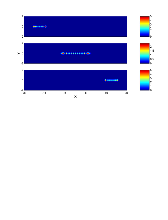
Figure 4: The vertical view of Fig. 3 with different line being corresponded to Fig. 3a, 3b and 3c respectively. Comparison between this with the figure 4 of Strecher’s article exhibits good agreement between them.

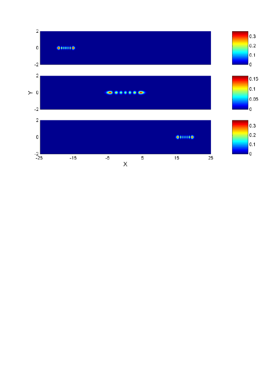
Figure 5: Transition of the matter-wave soliton trains. If the state of energy $E_{10}$ is disturbed by the interatomic interaction, the spontaneous transitions to the states of less average energy could occur. In Fig. 5 we show that the train consisting of eleven solitons is transformed into that of seven solitons for $n=6$. The different lines correspond to the times $\omega_{x}t=2\pi,\ 2.5\pi$ and $3\pi$ respectively.

Spontaneous transitions of the wave-packet trains In Strecher’s experiment on the matter-wave solitons, the trains with missing solitons were frequently observed, and this is resided in loss of condensed atoms. However, ”it is not clear whether this is because of a slow loss of atoms, or because of sudden loss of an individual soliton” [21]. According to transition theory of quantum-mechanical states, the non-interacting solitons could transit from higher-energy state to lower-energy state. The state function (2) and energy (5) imply that the lower-energy state describes less solitons. Therefore, even if the condensed atoms propagate without loss of number, some solitons may be suddenly lost, through spontaneous transitions of the macroscopic quantum states. Just after a transition, of course, the highness and width of each soliton should increase, since the atoms in lost solitons have entered the remainder solitons. The spontaneous transitions may be random and can be caused by some perturbations. We assume that under perturbation of the interatomic interaction the state of eleven solitons in Fig. 3 transits to the states with $n=6$ at $\omega_{x}t=2\pi$ as in the first line of Fig. 5 and propagates to $\omega_{x}t=2.5\pi$ and $\omega_{x}t=3\pi$ as in the second and third lines of Fig. 5.

Further considering the first order correction to the wave-packet trains from weak interaction and investigating transformation of the interaction from weak to strong will be very interesting. Because of the existence of arbitrary constants $A,\ B,\ \alpha,\ \beta,\ b_{0}$ and periodic functions $\rho(t),\ \theta(t)$, by using the complete solution (2) we can control motions of the BEC wave-packets. The theoretical control could indicate the directions of experimental operations that is important for real application, say, making an atomic soliton laser based on the bright soliton trains. In addition, the exact solution (2) could play an important role in treating various harmonically confined systems. For example, a single Paul trapped ion interacting with a harmonic potential, the state $\Psi_{1}$ of two wave-packets is similar to the Schr$\ddot{o}$dinger’s cat state [12], [13].

Acknowledgments This work was supported by the NNSF of China under Grant No. 10275023 and the NLMRAMP of China under Grant No. T152103, and by the Hubei Provincial Key Laboratory of Gravitation and Quantum Physics of China.

We adopt the natural unit with $m=\hbar=\omega_{x}=1$ and insert $\Psi_{n}=\psi_{n}(x,t)\psi_{y}(y)\psi_{z}(z)=(\sqrt{\pi}l_{r})^{-1}\exp[-(y^{2}+z^{2})/(2l_{r}^{2})]\psi_{n}(x,t),\ a=0$ into Eq. (1), producing the one dimensional equation of a harmonic oscillator

$$i\hbar\frac{\partial\psi_{n}}{\partial t}=-\frac{1}{2}\frac{\partial^{2}\psi_{n}}{\partial x^{2}}+\Big{[}\frac{1}{2}\omega_{x}^{2}x^{2}+\omega_{r}\Big{]}\psi_{n},\ \ \ \ \ \ \ \ \ \ \ \ \ \ \ \ \ \ \ \ \ \ \ \ \ (A1)$$

where units of $t$ and $x$ are $\omega_{x}^{-1}$ and $l_{x}$ respectively, $\omega_{r}$ is normalized by $\omega_{x}$ and appearance of the later is only formal, since its value has been fixed to 1. Let the solution of Eq. (A1) be in the form

$$\psi_{n}=a_{n}(t)H_{n}(\xi)\exp[b(t)x-c(t)x^{2}-f^{2}(t)/2],\ \ \xi=e(t)x-f(t)\ \ \ \ \ (A2)$$

with $a(t),\ b(t),\ c(t)$ being the complex functions of time and $e(t),\ f(t)$ the real functions. Applying Eq. (A2) to Eq. (A1), we arrive at the equation

$$e^{2}\frac{\partial^{2}H_{n}}{\partial\xi^{2}} + 2(be-i\dot{f}+i\dot{e}x-2cex)\frac{\partial H_{n}}{\partial\xi}$$

$$+2\Big{[}i\frac{\dot{a}_{n}}{a_{n}} - if\dot{f}+\frac{b^{2}}{2}-c-\omega_{r}+(i\dot{b}-2bc)x+\Big{(}2c^{2}-i\dot{c}-\frac{1}{2}\omega_{x}^{2}\Big{)}x^{2}\Big{]}H_{n}=0.\ \ \ (A3)$$

Noticing the Hermitian equation $\partial^{2}H_{n}/\partial\xi^{2}-2\xi\partial H_{n}/\partial\xi+2nH_{n}=0$, Eq. (A3) implies

$$i\dot{c} = 2c^{2}-\omega_{x}^{2}/2,\ \ i\dot{b}=2bc,\ \ i\dot{e}=2ce-e^{3},$$

$$i\dot{f} = be-e^{2}f,\ \ i\dot{a}_{n}/a_{n}=if\dot{f}-b^{2}/2+c+\omega_{r}+ne^{2}.\ \ \ \ \ \ \ \ \ \ (A4)$$

The first of Eq. (A4) is a complex Riccati equation, which can be changed into a complex equation of a classical harmonic oscillator

$$\ddot{\varphi}=-\omega_{x}^{2}\varphi,\ \ \ \ \ \ \ \ \ \ \ \ \ \ \ \ \ \ \ \ \ \ (A5)$$

through the function transformation $c=\dot{\varphi}/(2i\varphi)$. The general solution of Eq. (A5) is well-known that

$$\varphi=A\cos(\omega_{x}t+\alpha)+iB\cos(\omega_{x}t+\beta)=\rho(x,t)\exp[i\theta(x,t)],\ \ \ \ \ \ \ \ \ \ \ \ \ \ \ \ \ \ (A6)$$

where $A,\ B,\ \alpha$ and $\beta$ are arbitrary constants, the real functions $\rho(x,t)$ and $\theta(x,t)$ have been given by Eq. (3). Returning to the transformation between $\varphi$ and $c$ yields

$$c=\frac{\dot{\varphi}}{2i\varphi}=\frac{1}{2}\dot{\theta}-i\frac{\dot{\rho}}{2\rho}.\ \ \ \ \ \ \ \ \ \ \ \ \ \ \ \ \ \ \ \ \ \ (A7)$$

Substitution of Eq. (A6) into Eq. (A5) yields equations of the amplitude and phase as

$$\ddot{\theta}=-2\dot{\theta}\dot{\rho}/\rho,\ \ \ \ddot{\rho}=\rho\dot{\theta}^{2}-\omega_{x}^{2}\rho\ \ \ \ \ \ \ \ \ \ \ \ \ \ \ \ \ \ \ \ \ \ (A8)$$

with the first integrations

$$c_{0}=\rho^{2}\dot{\theta}=AB\omega_{x}\sin(\alpha-\beta),\ \ \ \ c_{1}=(\dot{\rho}^{2}+c_{0}^{2}/\rho^{2}+\rho^{2}\omega_{x}^{2})/2.\ \ \ \ \ \ \ \ \ \ \ \ \ \ \ \ \ \ \ \ \ \ (A9)$$

Combining Eqs. (A7) and (A6) with Eq. (A4) and applying the relation (A9), we easily obtain

$$b = b_{0}\frac{\exp(-i\theta)}{\rho},\ e=\frac{\sqrt{c_{0}}}{\rho}=\sqrt{\dot{\theta}},\ f=\frac{b_{0}}{\sqrt{c_{0}}}\cos\theta,$$

$$a_{n} = \frac{A_{0}}{\sqrt{\rho}}\exp\Big{(}-i\Big{[}\Big{(}\frac{1}{2}+n\Big{)}\theta+\omega_{r}t-\frac{b_{0}^{2}}{4c_{0}}\sin 2\theta\Big{]}\Big{)}.\ \ \ \ \ \ \ \ \ (A10)$$

Inserting these into Eq. (A2) leads to the axial solution $\psi_{n}(x,t)$, and the normalization condition $\int|\psi_{n}|^{2}dx=A_{0}^{2}\sqrt{c_{0}^{-1}}\int H_{n}^{2}(\xi)\exp(-\xi^{2})d\xi=A_{0}^{2}\sqrt{\pi c_{0}^{-1}}2^{n}n!=1$ gives the constant $A_{0}=[\sqrt{c_{0}}/(\sqrt{\pi}2^{n}n!)]^{1/2}$ such that Eq. (A2) becomes

$$\psi_{n}(x,t)=\Big{[}\frac{\sqrt{c_{0}}}{\sqrt{\pi}2^{n}n!\rho(t)}\Big{]}^{1/2}H_{n}(\xi)\exp\Big{[}-\frac{1}{2}\xi^{2}+i\Theta_{n}(x,t)\Big{]},\ \ \ \ \ \ \ \ \ (A11)$$

where the function $\Theta(x,t)$ has been written in Eq. (2). Combining this with the wave-function of transverse dimension and letting the unit of spatial coordinate return to original one, $x\rightarrow x/l_{x}$, we finally get the normalized 3D wave-function, as in Eq. (2).

Appendix B:  Proof of the Average Energy

Employing the Dirac’s symbols, ket and bra, from Eq. (A2) and the quantum-mechanical definition of average energy in state $\psi_{n}$ we perform the calculation

$$E_{n}=\langle\psi_{n}|i\frac{\partial}{\partial t}\psi_{n}\rangle=i\langle\psi_{n}|\frac{\dot{a}_{n}}{a_{n}}+(\dot{e}x-\dot{f})\frac{1}{H_{n}}\frac{\partial H_{n}}{\partial\xi}-(f\dot{f}-\dot{b}x+\dot{c}x^{2})|\psi_{n}\rangle.\ \ \ \ \ \ \ \ (A12)$$

Noticing the orthonormalization condition $\langle\psi_{n}|\psi_{n^{\prime}}\rangle=\delta_{nn^{\prime}}$ and the formulas

$$\xi=e(t)x-f(t),\ \ \xi\psi_{n}=\sqrt{n/2}\psi_{n-1}+\sqrt{(n+1)/2}\psi_{n+1},\$$

$$2\xi^{2}\psi_{n}=\sqrt{n(n-1)}\psi_{n-2}+(2n+1)\psi_{n}+\sqrt{(n+1)(n+2)}\psi_{n+2},$$

$$\frac{1}{H_{n}}\frac{\partial H_{n}}{\partial\xi}\psi_{n}=2n\frac{H_{n-1}}{H_{n}}\psi_{n}=\sqrt{2n}\psi_{n-1},\ \ \ \ \ \ \ \ \ \ \ \ \ \$$

we continue to compute the average energy

$$E_{n} = i\Big{(}\frac{\dot{a}_{n}}{a_{n}}-f\dot{f}\Big{)}+i\langle\psi_{n}|\sqrt{2n}\dot{e}\xi/e|\psi_{n-1}\rangle+i\langle\psi_{n}|\dot{b}x-\dot{c}x^{2}|\psi_{n}\rangle$$

$$= i\Big{(}\frac{\dot{a}_{n}}{a_{n}}-f\dot{f}+n\frac{\dot{e}}{e}-\frac{\dot{c}}{e^{2}}\Big{[}f^{2}+\Big{(}\frac{1}{2}+n\Big{)}\Big{]}\Big{)}+i\frac{\dot{b}f}{e}.$$

Applying Eqs. (A4) to the above equation results in

$$E_{n} = (2n+1)c+\omega_{r}-\frac{b^{2}}{2}-\Big{(}2c^{2}-\frac{\omega_{x}^{2}}{2}\Big{)}\Big{[}f^{2}+\Big{(}\frac{1}{2}+n\Big{)}\Big{]}\frac{1}{e^{2}}+2bc\frac{f}{e}.\ \ \ \ \ \ \ \ \ \ \ \ \ \ (A13)$$

Noticing Eqs. (A7), (A9) and (A10) we have

$$(2n+1)c-\Big{(}2c^{2}-\frac{\omega_{x}^{2}}{2}\Big{)}\Big{(}\frac{1}{2}+n\Big{)}\frac{1}{e^{2}}=\Big{(}\frac{1}{2}+n\Big{)}\frac{c_{1}}{c_{0}},\ \ 2bc\frac{f}{e}-\frac{b^{2}}{2}-\Big{(}2c^{2}-\frac{\omega_{x}^{2}}{2}\Big{)}\frac{f^{2}}{e^{2}}=\frac{b_{0}^{2}}{c_{0}}c_{2},\$$

$$c_{2}=\frac{\dot{\theta}}{2}+\Big{(}\frac{c_{1}}{c_{0}}-\dot{\theta}\Big{)}\cos^{2}\theta-\frac{\dot{\rho}}{\rho}\cos\theta\sin\theta.\ \ \ \ \ \ \ \ \ \ \ \ \ \ \ \ \ \ \ \ \ \ \ \ \ \$$

The third equation and Eqs. (A6) and (A9) imply

$$\frac{c_{2}}{\dot{\theta}} = \frac{c_{2}}{c_{0}}\rho^{2}=\frac{1}{2}-\cos^{2}\theta+\frac{c_{1}}{c_{0}^{2}}(\rho\cos\theta)^{2}-\frac{1}{c_{0}}(\rho\sin\theta)\dot{\rho}\cos\theta$$

$$= \frac{1}{2}-\cos^{2}\theta+\frac{c_{1}}{c_{0}^{2}}(\rho\cos\theta)^{2}-\frac{1}{c_{0}}(\rho\sin\theta)\Big{[}\frac{c_{0}}{\rho}\sin\theta-A\omega_{x}\sin(\omega_{x}t+\alpha)\Big{]}$$

so that we get

$$\frac{c_{2}}{c_{0}}[A^{2}\cos^{2}(\omega_{x}t+\alpha)+B^{2}\cos^{2}(\omega_{x}t+\beta)]\ \ \ \ \ \ \ \ \ \ \ \ \ \ \ \ \ \ \ \ \ \ \ \ \ \$$

$$=-\frac{1}{2}+\frac{c_{1}}{c_{0}^{2}}A^{2}\cos^{2}(\omega_{x}t+\alpha)+\frac{\omega_{x}}{c_{0}}AB\cos(\omega_{x}t+\beta)\sin(\omega_{x}t+\alpha).$$

Let the function of time be in the forms $\sin(2\omega_{x}t)$ and $\cos(2\omega_{x}t)$, and identify the corresponding coefficients of both sides, producing

$$c_{2}=\frac{A^{2}c_{1}}{(A^{2}+B^{2})c_{0}}.$$

Combining these with Eq. (13) leads to

$$E_{n}=\Big{(}\frac{1}{2}+n\Big{)}\frac{c_{1}}{c_{0}}+\omega_{r}+\frac{b_{0}^{2}}{c_{0}}c_{2},\ \ \ \ n=0,\ 1,\ 2,\ \cdots.$$

This is just the macroscopic quantum level (5).

References

[1] L.D. Landau and E.M. Lifshitz, Quantum
Mechanics, Nonrelativistic Theory (Butterworth-Heinemann, Oxford,
1977), Translated by J.B. Sykes and J.S. Bell.
[2] L. Schiff, Quantum Mechanics (McGraw-Hill, New York, 1957).
[3] J. Zeng, Quantum Mechanics(Science Press, Beijing, 1995), (in
Chinese).
[4] W.H. Steeb, Hilbert Spaces, Wavelets, Generalized Functions and Modern Quantum Mechanics (Kluwer Academic Publisher,
Dordrecht, 1998)
[5] W. Hai, M. Feng, X. Zhu, L. Shi, K. Gao and X. Fang, Phys. Rev. A61, 052105(2000).
[6] E. Schrdinger,
Naturwissenschaften, 14, 664(1926).
[7] J.R. Klauder and B. Skagerstam, Coherent states
(World Scientific Press, Singapore, 1985).
[8] S. Howard and S.K. Ray, Am. J. Phys., 55,
1109(1987).
[22] L. Khaykovich, F. Schreck, G. Ferrari, T. Bourdel, J. Cubizolles,
L. D. Carr, Y. Castin and C. Salomon, Science, 296, 1290(2002).
[23] E. Tiesinga, B. J. Verhaar, and H. T. C. Stoof, Phys. Rev. A47, 4114(1993).
[24] S. Inouye et al., Nature 392,151(1998).
[25] U. Al Khawaja, H.T. C. Stoof, R.G. Hulet, K. E. Strecker, and
G. B. Partridge, Phys. Rev. Lett., 89, 200404(2002).
[26] J. Denschlag, J. E. Simsarian, D. L.
Feder, Charles W. Clark, L. A. Collins, J. Cubizolles, L. Deng, E.
W. Hagley, K. Helmerson, W. P. Reinhardt, S. L. Rolston, B. I.
Schneider, W. D. Phillips, Science, 287, 97(2000).
[27] M. Greiner, O. Mandel, T. W. Hansch and I.
Bloch, Nature, 419, 51(2002).
[28] C. A. Sackett, J. M. Gerton, M. Welling, and R. G.
Hulet, Phys. Rev. Lett., 82, 876(1999).
[29] H. Saito and M. Ueda, Phys. Rev. Lett., 86, 1406(2001).
[30] W. Hai, C. Lee, G. Chong and L. Shi, Phys. Rev. E66, 026202(2002).