Distillation Protocols for Mixed States of Multilevel Qubits and
the Quantum Renormalization Group

Abstract

We study several properties of distillation protocols to purify multilevel qubit states (qudits) when applied to a certain family of initial mixed bipartite states. We find that it is possible to use qudits states to increase the stability region obtained with the flow equations to distill qubits. In particular, for qutrits we get the phase diagram of the distillation process with a rich structure of fixed points. We investigate the large-$D$ limit of qudits protocols and find an analytical solution in the continuum limit. The general solution of the distillation recursion relations is presented in an appendix. We stress the notion of weight amplification for distillation protocols as opposed to the quantum amplitude amplification that appears in the Grover algorithm. Likewise, we investigate the relations between quantum distillation and quantum renormalization processes.

I Introduction

The experimental analysis of the intriguing properties of entanglement in quantum mechanics requires the availability of stable sources of entanglement. Despite the nice properties exhibited by entanglement, it has the odd behaviour of degrading by the unavoidable contact with the external environment. Thus, for the entanglement to be assessed as a precious mean, we must devise some method to pump it up to the entanglement source in order to sustain a prescribed degree of entanglement that we may need whether for quantum communication protocols (teleportation, cryptography, dense coding) or quantum computing (algorithmics) (for a review see review1 , review2 and references therein).

Quantum distillation or purification protocols are precisely those methods, that have been devised to regenerate entanglement leakages of an entanglement source. Here we are interested in the purification of mixed states of bipartite type, having in mind the realization of a communication protocol by two parties, Alice and Bob. The seminal work of bennett1 has provided us with a standard distillation method that has been the focus to developing more protocols with the aim at improving its original performances. We shall refer to this distillation protocol as the BBPSSW protocol. There are feasible experimental proposals for this type of protocols using polarization beam splitters (PBS) zeilinger1 . Likewise, there also exist methods for the distillation of pure states gisin that have been implemented experimentally gisin3 .

In addition to the initial purpose for which the quantum distillation protocols were devised, they have found another very important application in connection to the problem of quantum error correction: quantum information needs to be protected from errors even more than classical information due to its tendency to become decoherent. To avoid these errors, one can resort to the ideas of quantum error correction codes shor , steane and fault-tolerant quantum computation gottesman , preskill . However, entanglement purification is another alternative to decoherence which gives a more powerful way of dealing with errors in quantum communication bennett2 .

In a typical quantum communication experiment, Alice and Bob are two spatially separated parties sharing pairs of entangled qubits. The type of operations allowed on these qubits are denoted as LOCC (Local Operations and Classical Communication): they comprise local unitary operators $U_{\rm A}\otimes U_{\rm B}$ on each side, local quantum measurements and communication of the measurement results through a classical channel. These local quantum operations will suffer from imperfections producing local errors. Futhermore, Alice and Bob will also face transmission errors in their quantum channels due to dissipation and noise. To overcome these difficulties, they will have to set up an entanglement purification method. In short, a protocol like the BBPSSW creates a reduced set of maximally entangled pairs (within a certain accuracy) out of a larger set of imperfectly entangled pairs: entanglement is created at the expense of wasting extra pairs. The degree of purity of a mixed entangled pair is measured in terms of its fidelity with respect to a maximally entangled pure pair, which is the focus of the purification protocol. After the BBPSSW protocol, a new distillation protocol was introduced in qpa by the name of Quantum Privacy Amplification(QPA) which converges much faster to the desired fidelity chiara1 , chiara2 . Other protocols known as quantum repeaters repeaters-pur , repeaters-com allow us to stablish quantum communication over long distances by avoiding absortion or depolarization errors that scale exponentially with the length of the quantum channel.

The advantages of dealing with $D$-dimensional or multilevel quantum states (qudits) instead of qubits are quite apparent: an increase in the information flux through the communication channels that could speed up quantum cryptography, etc. pasqui1 , pasqui2 , karlson . Thus, it has been quite natural to propose extensions of the purification protocols for qudits. One of the proposals horodeckis relies on an extension of the CNOT gate that is unitary, but not Hermitian. Recently, another very nice proposal has been introduced gisin1 , gisin2 based on a generalization of the CNOT gate that is both unitary and Hermitian and gives a higher convergence. In this paper we make a study of the new purification protocols of gisin1 , gisin2 when they are applied to mixed bipartite states of qudits that are not of the Werner form. In this way, we combine some of the tools employed by the QPA protocols qpa with the advantages of the new methods.

This paper is organized as follows: in Sect. II we review simple distillation protocols for qubits not in Werner states and we generalize them for the purification of any of the Bell states. In Sect. III we extend the previous protocols to deal with multilevel qubits and obtain several results like an improvement in the size of the stability fidelity basin, analytical formulas for the distillation flows, phase diagrams, etc. In Sect. IV we apply the distillation protocols for the purification of non-diagonal mixed states that are more easily realized experimentally. In Sect. V we study the large-$D$ limit of these protocols. In Sect. VI we present a detailed investigation of the relationships between quantum distillation protocols and renormalization methods for quantum lattice Hamiltonians. Section VII is devoted to conclusions. In appendix A we find the general solution for the distillation recursion relations used in the text in the general case of qudits.

II Simple Distillation Protocols with Qubits

Our starting point is the orthonormal basis of Bell states formed by the first qubit belonging to Alice and the second to Bob:

$$\begin{split}|\Phi^{\pm}\rangle&:=\frac{1}{\sqrt{2}}[|00\rangle\pm|11\rangle]\\ |\Psi^{\pm}\rangle&:=\frac{1}{\sqrt{2}}[|01\rangle\pm|10\rangle]\end{split}$$ (1)

We shall use the word “simple” applied to the distillation protocols to denote that the mixed state we shall be dealing with is made up of a combination of one state in the set $S:=\{|\Phi^{+}\rangle,|\Phi^{-}\rangle\}$ of Bell states that have coincident bits in Alice’s and Bob’s qubits, with another state in the set $A:=\{|\Psi^{+}\rangle,|\Psi^{-}\rangle\}$ of Bell states that do not have coincidences. Thus, we have 4 possible combinations to do this type of entanglement distillation.

To begin with, we shall choose the following mixed state in order to set up a simple distillation protocol

$$\rho_{++}:=F|\Phi^{+}\rangle\langle\Phi^{+}|+(1-F)|\Psi^{+}\rangle\langle\Psi^{+}|$$ (2)

Alice and Bob will also need to apply the CNOT gate defined as usual

$$U_{\rm CNOT}|i\rangle|j\rangle:=|i\rangle|i\oplus j\rangle,\ i,j=0,1.$$ (3)

The distillation protocol can be arranged into a set of 5 instructions or steps bennett1 ,qpa ,chiara2 :

Distillation Protocol for Qubits

1. Set up $\rho\longrightarrow\rho\otimes\rho$ with fidelity $F$.

2. Apply bilateral CNOT gate: $U_{\rm BCNOT}$.

3. Alice and Bob measure target qubits.

4. Classical communication of results: retain coincidences ($0_{A}0_{B}$ or $1_{A}1_{B}$).

5. Go to step 1) with $\rho^{\prime}$ with fidelity $F^{\prime}>F$.

The simplicity of this protocol also relies on the fact that we do not need any depolarization step, as it is the case when dealing with Werner states bennett1 . In Fig. 1 we show a schematic picture of a single aplication of the purification method. Let us comment on the outcomes corresponding to the most relevant steps in this protocol. After step 1/, the 4-quit mixed state $\rho\otimes\rho$ shared by Alice and Bob reads as follows

$$\begin{split}&\rho_{++}\otimes\rho_{++}=F^{2}|\Phi^{+}\Phi^{+}\rangle\langle\Phi^{+}\Phi^{+}|\\ &+F(1-F)[|\Phi^{+}\Psi^{+}\rangle\langle\Phi^{+}\Psi^{+}|+|\Psi^{+}\Phi^{+}\rangle\langle\Psi^{+}\Phi^{+}|]\\ &+(1-F)^{2}|\Psi^{+}\Psi^{+}\rangle\langle\Psi^{+}\Psi^{+}|\end{split}$$ (4)

In step 2/, Alice and Bob apply bilaterally the CNOT gate taking their first qubit as source and their second qubit as target, i.e., qubits first and third are source qubits while qubits second and fourth are target qubits. To obtain the transformed mixed state we must determine the action of the bilateral CNOT gate $U_{\rm BCNOT}$ bennett1 on the states of the form $|\varphi_{A}\varphi_{B}\rangle$. The results of this computation are shown in Table 1. With the help of this table we find

$$\begin{split}&U_{\rm BCNOT}\rho_{++}\otimes\rho_{++}U_{\rm BCNOT}=F^{2}|\Phi^{+}\Phi^{+}\rangle\langle\Phi^{+}\Phi^{+}|\\ &+F(1-F)[|\Phi^{+}\Psi^{+}\rangle\langle\Phi^{+}\Psi^{+}|+|\Psi^{+}\Psi^{+}\rangle\langle\Psi^{+}\Psi^{+}|]\\ &+(1-F)^{2}|\Psi^{+}\Phi^{+}\rangle\langle\Psi^{+}\Phi^{+}|\end{split}$$ (5)

\psfrag{A}[Bc][Bc][1][0]{Alice}\psfrag{B}[Bc][Bc][1][0]{Bob}\psfrag{F}[Bc][Bc][1][0]{$F$}\psfrag{G}[Bc][Bc][1][0]{$F$}\psfrag{H}[Bc][Bc][1][0]{$F$}\psfrag{I}[Bc][Bc][1][0]{$F$}\psfrag{C}[Bc][Bc][1][0]{CNOT}\psfrag{D}[Bc][Bc][1][0]{CNOT}\psfrag{P}[Bc][Bc][1][0]{Quantum}\psfrag{Q}[Bc][Bc][1][0]{Distillation}\psfrag{J}[Bc][Bc][1][0]{$F^{\prime}>F$}\psfrag{K}[Bc][Bc][1][0]{$F^{\prime}>F$}\includegraphics[width=170.71652pt]{protocolqubits.eps}

Figure 1: Schematic representation of the distillation protocol by Alice and Bob. Originally, two pairs of shared entangled qubits represented by enclosed dots are transformed into a single pair of higher purity (doubly enclosed dots).

After steps 3/ and 4/, Alice and Bob measure their target qubits and retain their source qubit whenever they find, via classical communication, the same results: either $0_{A}0_{B}$ or $1_{A}1_{B}$. This fact selects the state $|\Phi^{+}\rangle$ as the only admissible possibility for the target state. Thus, only the first and third terms in the RHS of (5) survive to this process and the resulting 2-qubit state $\rho^{\prime}_{++}$ is again of the same form as the original starting state (2) in step 1/, but with a higher fidelity $F^{\prime}>F$. In fact, we get

$$\rho^{\prime}_{++}:=F^{\prime}|\Phi^{+}\rangle\langle\Phi^{+}|+(1-F^{\prime})|\Psi^{+}\rangle\langle\Psi^{+}|$$ (6)

with the new fidelity being

$$F^{\prime}=\frac{F^{2}}{F^{2}+(1-F)^{2}}$$ (7)

This relation defines a recursion scheme for entanglement purification: starting with say $N_{P}$ pairs of Bell states of fidelity $F$, after every application of the whole protocol we obtain $\frac{N_{P}}{2}$ pairs of higher fidelity $F^{\prime}>F$. Thus, purification is achieved at the expense of halving the number of Bell pairs. The fixed points $F_{c}$ of the recursion relation (7) are defined as $F^{\prime}(F_{c}):=F_{c}$ and they are given by $F_{c}=0,\textstyle\frac{1}{2},1$. The fixed points $F_{c}=0,1$ are stable, while $F_{c}=\textstyle\frac{1}{2}$ is unstable. The best way to recast these qualitative properties of the flow equation for the fidelities (7) is to draw the corresponding flow diagram as shown in Fig. 2.

$|\varphi_{A}\rangle|\varphi_{B}\rangle$	$U_{\rm BCNOT}|\varphi_{A}\rangle|\varphi_{B}\rangle$
$|\Phi^{+}\rangle|\Phi^{+}\rangle$	$|\Phi^{+}\rangle|\Phi^{+}\rangle$
$|\Phi^{+}\rangle|\Psi^{+}\rangle$	$|\Phi^{+}\rangle|\Psi^{+}\rangle$
$|\Psi^{+}\rangle|\Phi^{+}\rangle$	$|\Psi^{+}\rangle|\Psi^{+}\rangle$
$|\Psi^{+}\rangle|\Psi^{+}\rangle$	$|\Psi^{+}\rangle|\Phi^{+}\rangle$

Table 1: This table shows the results of applying the bilateral CNOT gate to certain pairs of Bell states needed to distillation.

\psfrag{0}[Bc][Bc][1][0]{0}\psfrag{1}[Bc][Bc][1][0]{1}\psfrag{2}[Bc][Bc][1][0]{$F_{c}$}\psfrag{c}[Bc][Bc][1][0]{$\textstyle\frac{1}{2}$}\psfrag{g}[Bc][Bc][1][0]{$F$}\includegraphics[width=170.71652pt]{flowdiagram.eps}

Figure 2: Flow diagram for the fidelity $F$ of the distillation protocol given by the recursion relation (7).

Next, we may wonder whether it is possible to devise distillation protocols for the three possible combinations of Bell states, namely,

$$\begin{split}\rho_{+-}&:=F|\Phi^{+}\rangle\langle\Phi^{+}|+(1-F)|\Psi^{-}\rangle\langle\Psi^{-}|\\ \rho_{-+}&:=F|\Phi^{-}\rangle\langle\Phi^{-}|+(1-F)|\Psi^{+}\rangle\langle\Psi^{+}|\\ \rho_{--}&:=F|\Phi^{-}\rangle\langle\Phi^{-}|+(1-F)|\Psi^{-}\rangle\langle\Psi^{-}|\end{split}$$ (8)

We can answer this question affirmatively by computing the action of the bilateral CNOT gate on the tensor product of these mixed states (8). With a similar analysis which has led us to Table 1 bennett1 , we obtain

$$\begin{split}&U_{\rm BCNOT}\rho_{+-}\otimes\rho_{+-}U_{\rm BCNOT}=F^{2}|\Phi^{+}\Phi^{+}\rangle\langle\Phi^{+}\Phi^{+}|\\ &+F(1-F)[|\Phi^{-}\Psi^{-}\rangle\langle\Phi^{-}\Psi^{-}|+|\Psi^{-}\Psi^{+}\rangle\langle\Psi^{-}\Psi^{+}|]\\ &+(1-F)^{2}|\Psi^{+}\Phi^{-}\rangle\langle\Psi^{+}\Phi^{-}|\\ &U_{\rm BCNOT}\rho_{-+}\otimes\rho_{-+}U_{\rm BCNOT}=F^{2}|\Phi^{+}\Phi^{-}\rangle\langle\Phi^{+}\Phi^{-}|\\ &+F(1-F)[|\Phi^{-}\Psi^{+}\rangle\langle\Phi^{-}\Psi^{+}|+|\Psi^{-}\Psi^{-}\rangle\langle\Psi^{-}\Psi^{-}|]\\ &+(1-F)^{2}|\Psi^{+}\Phi^{+}\rangle\langle\Psi^{+}\Phi^{+}|\\ &U_{\rm BCNOT}\rho_{--}\otimes\rho_{--}U_{\rm BCNOT}=F^{2}|\Phi^{+}\Phi^{-}\rangle\langle\Phi^{+}\Phi^{-}|\\ &+F(1-F)[|\Phi^{+}\Psi^{-}\rangle\langle\Phi^{+}\Psi^{-}|+|\Psi^{+}\Psi^{-}\rangle\langle\Psi^{+}\Psi^{-}|]\\ &+(1-F)^{2}|\Psi^{+}\Phi^{-}\rangle\langle\Psi^{+}\Phi^{-}|\end{split}$$ (9)

We now realize that if we proceed to measure the target bits and classical communicate the results, we do not end up with the same type of mixed state as we had started with. That is, the protocol as it stands is not valid since it does not yield invariant mixed states. This problem has a solution provided we introduce an additional step prior to the measurement of the target qubits by Alice and Bob. This additional step corresponds to a local unitary operation $U_{A}\otimes U_{B}$ performed by Alice and Bob on their source qubits. The form of this local unitary depends on the mixed state we are distilling. We find the following results:

Step $2^{\prime}$. Alice and Bob apply a local unitary transformation $U_{A}\otimes U_{B}$ to their source qubits:

For $\rho_{+-}$, $U_{A}=\textstyle\frac{1}{2}(1+\mathord{\rm i})(\sigma_{x}+\sigma_{y})$, $U_{B}=\textstyle\frac{1}{2}(1-\mathord{\rm i})(\sigma_{x}-\sigma_{y})$.

For $\rho_{-+}$, $U_{A}=U_{B}=\textstyle\frac{1}{2}(1+\mathord{\rm i})(\sigma_{x}+\sigma_{y})$.

For $\rho_{--}$, $U_{A}=\sigma_{z}$, $U_{B}=1$.

After this extra step, we can guarantee that the resulting 4-qubit mixed state has the appropriate Bell pairs at the source qubits so as to produce the same original state, once steps 3/ and 4/ are performed. Moreover, it is straightforward to prove that the new fidelity for these 3 protocols is also given by the same recursion relation (7) as in the first protocol.

Finally, if the constraint that the state of fidelity $F$ must be a $\Phi^{\pm}$ state is relaxed, then there are two additional possible mixed states whose analysis can be carried out in a similar fashion.

III Multilevel Extensions of Distillation Protocols

In order to generalize the simple distillation protocol of the previous section to the case of qudits, we must notice that the two main ingredients in that distillation protocol are:

i) the CNOT gate,

ii) the Bell states (1).

Regarding the CNOT gate, the extension of this gate to deal with qudits is not unique. As has been noted in gisin1 ,gisin2 , the CNOT gate for qubits (3) has 3 properties that make it special, namely

$$\begin{split}U_{\rm CNOT}^{{\dagger}}=U_{\rm CNOT}^{-1},\\ U_{\rm CNOT}^{{\dagger}}=U_{\rm CNOT},\\ i\oplus j=0\Leftrightarrow i=j.\end{split}$$ (10)

The extension of the CNOT gate for qudits that satisfies these 3 properties (10) is given by gisin1 ,gisin2

$$U_{\rm CNOT}|i\rangle|j\rangle:=|i\rangle|i\ominus j\rangle,\ i,j=0,\ldots,D-1$$ (11)

where $i\ominus j:=i-j,{\rm mod}\ D$, denotes substraction modulus $D$. This is the definition that we shall adopt throughout this paper, unless otherwise stated.

As for the higher-dimensional extension of Bell states (1), we shall also take the following generalization gisin1 ,gisin2

$$|\Psi_{kj}\rangle:=U_{\rm CNOT}\left[(U_{\rm F}|k\rangle)\otimes|j\rangle\right],\ k,j=0,\ldots,D-1$$ (12)

where $U_{\rm F}$ is the quantum Fourier transform (QFT)

$$U_{\rm F}|k\rangle:=\frac{1}{\sqrt{D}}\sum_{y=0}^{D-1}\mathord{\rm e}^{\frac{2\pi\mathord{\rm i}ky}{D}}|y\rangle,$$ (13)

which reduces to the Hadamard gate when dealing with qubits ($D=2$). As a matter of fact, we can readily check that for the special case of qubits $D=2$ we recover the standard Bell pairs (1) in the following form

$$\begin{split}|\Psi_{00}\rangle=|\Phi^{+}\rangle,&|\Psi_{01}\rangle=|\Psi^{+}\rangle,\\ |\Psi_{10}\rangle=|\Phi^{-}\rangle,&|\Psi_{11}\rangle=|\Psi^{-}\rangle\end{split}$$ (14)

Moreover, using the generalized CNOT gate (11), the generalized Bell states are given by

$$|\Psi_{kj}\rangle=\frac{1}{\sqrt{D}}\sum_{y=0}^{D-1}\mathord{\rm e}^{\frac{2\pi\mathord{\rm i}ky}{D}}|y\rangle|y\ominus j\rangle.$$ (15)

With these extensions of the CNOT gate and the Bell states, we can set up a generalization of the simple distillation protocols of Sect. II for qudit states. These protocols have the same 5 steps as before.

Step 1/. We shall assume a general diagonal mixed state of the form

$$\begin{split}\rho&:=\sum_{k,j=0}^{D-1}q_{kj}|\Psi_{ij}\rangle\langle\Psi_{ij}|,\\ 1&=:\sum_{k,j=0}^{D-1}q_{kj},\end{split}$$ (16)

where $q_{kj}$ are normalized probabilities. For non-diagonal mixed states, we refer to Sect. IV. Then, Alice and Bob share pairs $\rho\times\rho$ of these states (16).

Step 2/. Alice and Bob apply bilaterally the generalized CNOT gate (11). To know the result of this operation on the state (16) we need a previous result about the action of the gate $U_{\rm BCNOT}$ on pairs of generalized Bell states (12). After some algebra, we arrive at the following expression

$$U_{\rm BCNOT}|\Psi_{kj}\rangle|\Psi_{k^{\prime}j^{\prime}}\rangle=|\Psi_{k\oplus k^{\prime},j}\rangle|\Psi_{D\ominus k^{\prime},j\ominus j^{\prime}}\rangle$$ (17)

This is a fundamental result for it means that the space of two-pairs of generalized Bell states is invariant under the action of the generalized bilateral CNOT gate. This is a very nice result that condenses in a single formula all the possibilities for the outcome of the action of the CNOT gates on Bell states, in particular, the whole table employed by Bennett et al. in bennett1 for the case of qubits is contained in equation (17). This property is essential in order to have a closed distillation protocol. Actually, it would have been enough to have obtained only the source qubits as generalized Bell states.

Then, with the help of this property (17) we obtain the action of $U_{\rm BCNOT}$ on pairs of $\rho$ states, as follows

$$\begin{split}&U_{\rm BCNOT}\rho\otimes\rho U_{\rm BCNOT}=\sum_{k,j=0}^{D-1}\sum_{k^{\prime},j^{\prime}=0}^{D-1}q_{k\ominus k^{\prime},j}q_{k^{\prime}j^{\prime}}\\ &|\Psi_{kj}\Psi_{D\ominus k^{\prime},j\ominus j^{\prime}}\rangle\langle\Psi_{kj}\Psi_{D\ominus k^{\prime},j\ominus j^{\prime}}|\end{split}$$ (18)

We see that this state is already of the same form in the source qubits as the original $\rho$ (16).

Step 3/. Alice and Bob measure their target qubits in (18). To see the result of this measurement, let us write the explicit form of the target qubits, namely

$$\Psi_{D\ominus k^{\prime},j\ominus j^{\prime}}=\frac{1}{\sqrt{D}}\sum_{z=0}^{D-1}\mathord{\rm e}^{\frac{-2\pi\mathord{\rm i}k^{\prime}z}{D}}|z\rangle|z\ominus(j\ominus j^{\prime})\rangle.$$ (19)

Therefore, coincidences between Alice’s and Bob’s target qubits will happen only when the following condition is satisfied

$$z=z\ominus(j\ominus j^{\prime})\Longleftrightarrow j=j^{\prime}.$$ (20)

Step 4/. After their measurement, Alice and Bob communicate classically their result so that they retain the resulting source Bell pairs only when they have coincidences, and discard them otherwise. The resulting net effect of this process is to produce a Kronecker delta function $\delta_{jj^{\prime}}$ in the target qubits. More precisely, the resulting unnormalized mixed state is given by

$$\rho^{\prime}\sim\sum_{k,j=0}^{D-1}\sum_{k^{\prime},j^{\prime}=0}^{D-1}q_{k\ominus k^{\prime},j}q_{k^{\prime}j^{\prime}}\delta_{jj^{\prime}}|\Psi_{kj}\rangle\langle\Psi_{kj}|.$$ (21)

Therefore, we end up with a diagonal mixed state of the same form as the starting one

$$\rho^{\prime}=\sum_{k,j=0}^{D-1}q^{\prime}_{kj}|\Psi_{kj}\rangle\langle\Psi_{kj}|.$$ (22)

with the new probabilities given by

$$q^{\prime}_{kj}=\frac{\sum_{k^{\prime}=0}^{D-1}q_{k\ominus k^{\prime},j}q_{k^{\prime}j}}{\sum_{k,j=0}^{D-1}\sum_{k^{\prime}=0}^{D-1}q_{k\ominus k^{\prime},j}q_{k^{\prime}j}}.$$ (23)

This is a generalized recursion relation that includes eq. (7) as a particular instance.

Step 5/. Alice and Bob start all over again the same process with the initial state now being $\rho^{\prime}$ in (22-23).

The nice feature of these generalized distillation protocols for dealing with qudits is the fact that we have at our disposal explicit analytical formulas (23) for the evolution (flow) of the different weights (probabilities) of the generalized mixed states to be purified. As these distillation protocols are too general, it is worthwhile to consider some particular cases of interest separately. The general solution to the distillation recursion relations (23) is presented in the appendix A. We hereby provide the following analysis of some examples:

i). Let us investigate the closest generalization of the simple protocols introduced in Sect. II. Thus, let us consider the following type of initial mixed state

$$\begin{split}\rho&:=\sum_{i=0}^{M}q_{i}|\Psi_{0i}\rangle\langle\Psi_{0i}|,\ M\leq D-1,\\ 1&=:\sum_{i=0}^{M}q_{i},\ q_{i}\geq 0,\end{split}$$ (24)

This corresponds to working with the subset of all possible generalized Bell states of the form $\{|\Psi_{0i}\rangle\}_{i=0}^{D-1}$. Interestingly enough, this includes the case of the state $\rho_{++}$ in (2) for $D=2$. The recursion relations (23) for this special subset of states takes the following simpler form

$$q^{\prime}_{i}=\frac{q_{i}^{2}}{\sum_{j=0}^{M}q_{j}^{2}}.$$ (25)

For $M=2$, i.e., considering a mixed state formed of just two Bell states of the form $|\Psi_{0i}\rangle$, the protocol has the following recursion relation

$$q^{\prime}_{i}=\frac{q_{i}^{2}}{q_{i}^{2}+(1-q_{i})^{2}},$$ (26)

where here the index $i$ stands for any possible pair of Bell states of the type $|\Psi_{0i}\rangle$. In other words, we have found a direct $D$-dimensional generalization of the distillation protocols for qubits in Sect. II, with $q_{i}:=F$.

ii). For $M=D-1$ and taking $q_{0}:=F$ and $q_{i}:=\frac{1-F}{D-1},i=1,\ldots,D-1$ we can find a more advantageous protocol than the previous one. In fact, in this case we find that

$$q^{\prime}_{0}:=F^{\prime}=\frac{F^{2}}{F^{2}+\frac{(1-F)^{2}}{D-1}}.$$ (27)

The fixed points of this recursion relation are now given by $F_{c}=0,\frac{1}{D},1$. Despite being a non-linear recursion relation, (27) admits an explicit analytical solution for the general term of the series $F_{k}$ given by

$$F_{k}=\frac{F^{(2^{k})}}{F^{(2^{k})}+(D-1)\left[\frac{1-F}{D-1}\right]^{(2^{k})}},\ k\geq 1,F_{0}:=F.$$ (28)

From this solution, we inmediately find that the fixed points $F_{c}=0,1$ are stable while $F_{c}=\frac{1}{D}$ is unstable.

In Fig. 3 we plot the function $F^{\prime}=F^{\prime}(F)$ for several values of the dimension $D$. From the analysis of these curves we inmediately obtain the corresponding flow diagram that we represent in Fig. 4. We check that for $D=2$ we recover the flow diagram corresponding to standard qubits (Fig. 2).

\psfrag{x}[Bc][Bc][1][0]{$F$}\psfrag{y}[Bc][Bc][1][0]{$F^{\prime}$}\includegraphics[scale={0.5}]{recursionFD2.eps}

Figure 3: Plots of the distilled fidelities $F^{\prime}$ as a function of the original fidelity $F$ for several values of the dimension $D$ of the qudits: $D=2,4,10$.

\psfrag{0}[Bc][Bc][1][0]{0}\psfrag{1}[Bc][Bc][1][0]{1}\psfrag{2}[Bc][Bc][1][0]{$F_{c}$}\psfrag{c}[Bc][Bc][1][0]{$\frac{1}{D}$}\psfrag{g}[Bc][Bc][1][0]{$F$}\includegraphics[width=170.71652pt]{flowdiagramD.eps}

Figure 4: Flow diagram for the fidelity $F$ of the generalized distillation protocol for qudits given by the recursion relation (27).

We see from Fig. 4 that the stability basin is increased with respect to the case of standard qubits, as in Fig. 2. This means that we can start with a mixed state having a fidelity $F$ with respect to the Bell state $|\Psi_{00}\rangle$ lower that $\textstyle\frac{1}{2}$ and we still will succeed in purifiying that state towards fidelity close to 1. Thus, we have found that it is more advantageous to distill a given Bell state $|\Psi_{00}\rangle$ if we prepare the mixed state $\rho$ in (24) in the form

$$\rho:=F|\Psi_{00}\rangle\langle\Psi_{00}|+\frac{1-F}{D-1}\sum_{i=1}^{D-1}|\Psi_{0i}\rangle\langle\Psi_{0i}|,$$ (29)

rather than using just one single of those states

$$\rho:=F|\Psi_{00}\rangle\langle\Psi_{00}|+(1-F)|\Psi_{0i}\rangle\langle\Psi_{0i}|,\ i\neq 0.$$ (30)

We may wonder how is it likely for Alice and Bob to obtain the same values (coincidences) after measuring the target qudits in the step 3/ of the distillation protocol. Let us denote by ${\cal P}_{\rm AB}$ this probability which will depend on the value $F$ of the fidelity. From equations (21) and (27) we find this probability of coincidences to be

$${\cal P}_{\rm AB}(F)=F^{2}+\frac{(1-F)^{2}}{D-1}.$$ (31)

The minimum of this probability is at $F_{0}=\frac{1}{D}$ and its value is ${\cal P}_{\rm AB}(\frac{1}{D})=\frac{1}{D}$. Likewise, ${\cal P}_{\rm AB}(1)=1$. Thus, we find that the probability is lower and upper bounded as ${\frac{1}{D}\leq\cal P}_{\rm AB}(F)\leq F$ for $F\in[\frac{1}{D},1]$.

One is also interested in knowing the number of steps $K(\epsilon,F_{0})$ needed to achieve a certain final fidelity close to 1, say $1-\epsilon$, starting from an appropriate initial fidelity $F_{0}>\frac{1}{D}$. This number can be computed from our analytical solution (28) from the condition

$$F_{K(\epsilon,F_{0})}:=1-\epsilon.$$ (32)

Thus, we find the following analytical formula for the number of steps needed to obtain a certain degree of fidelity $\epsilon$ as a function of the initial fidelity $F_{0}>\frac{1}{D}$,i.e.,

$$K(\epsilon,F_{0})=\left\lceil\log_{2}\left(\frac{\ln(\frac{\epsilon}{(1-\epsilon)(D-1)})}{\ln(\frac{1-F_{0}}{(D-1)F_{0}})}\right)\right\rceil.$$ (33)

\psfrag{x}[Bc][Bc][1][0]{$F_{0}$}\psfrag{y}[Bc][Bc][1][0]{$K$}\includegraphics[width=227.62204pt]{iterations2.eps}

Figure 5: Plot of the number of iterations $K(\epsilon,F_{0})$ (33) to achieve a final fidelity of $F=0.99$ as a function of the initial fidelity $F_{0}$ and for several values of the dimension $D$ of the qudits: $D=2,4,10$.

In Fig. 5 we plot the number of iterations (33) for a given value of the final fidelity $1-\epsilon$ that we take as the fixed value of $0.99$, and then we find how is the dependence on the initial fidelity $F_{0}$. We see that for a given admissible value of $F_{0}$, the lowest number of iterations corresponds to the protocol with the higher value of the qudits dimension $D$:

$$K(\epsilon_{0},F_{0})_{D_{1}}\geq K(\epsilon_{0},F_{0})_{D_{2}},\ {\rm for}\ D_{1}>D_{2}.$$ (34)

iii). For qutrits, $D=3$, the most general diagonal mixed state with the allowed Bell states taking values on the set $\{|\Psi_{0i}\rangle\}$ is

$$\begin{split}\rho&:=q_{0}|\Psi_{00}\rangle+q_{1}|\Psi_{01}\rangle+q_{2}|\Psi_{02}\rangle\\ 1&=:q_{0}+q_{1}+q_{2}\end{split}$$ (35)

Let us assume that the state we want to purify is $|\Psi_{00}\rangle$. Now, our recursion relation for our fidelity $q_{0}$ depends on two variables, namely,

$$q^{\prime}_{0}=\frac{q_{0}^{2}}{q_{0}^{2}+q_{1}^{2}+(1-q_{0}-q_{1})^{2}},$$ (36)

and a similar equation for $q_{1}$ with $q_{0}\leftrightarrow q_{1}$. In Fig. 6 the dependence of the function fidelity $q^{\prime}_{0}=q^{\prime}_{0}(q_{0},q_{1})$ for qutrits is plotted. We observe that it is a monotonous incresing function which gurantees that the initial fidelity will flow towards 1, under certain conditions.

\psfrag{x}[Bc][Bc][1][0]{$q_{0}$}\psfrag{y}[Bc][Bc][1][0]{$q_{1}$}\psfrag{z}[Bc][Bc][1][0]{$q^{\prime}_{0}$}\includegraphics[width=227.62204pt]{qutrits3.eps}

Figure 6: The desired fidelity $q^{\prime}_{0}$ for amplification after a single application of the distillation protocol for qutrits (36) as a function of the previous fidelitites $q_{0},q_{1}$.

To find these conditions, we find that the set of fixed points of these recursion relations is given by

$$(q_{0},q_{1})_{c}=\{(0,0),(\textstyle\frac{1}{2},0),(0,\textstyle\frac{1}{2}),(\frac{1}{3},\frac{1}{3}),(\textstyle\frac{1}{2},\textstyle\frac{1}{2}),(1,0),(0,1)\}.$$

We have also found the flow diagram associated to these recursion relations which is now two-dimensional and we show it in Fig. 7. From this diagram we see that the purification protocol is successful in arriving to the maximum fidelity $q_{0}=1$ provided the initial fidelity lies in the stability basin of the fixed point $(1,0)$ which is given by the trapezoid formed by the set of points $(\textstyle\frac{1}{2},\textstyle\frac{1}{2}),(\frac{1}{3},\frac{1}{3}),(\textstyle\frac{1}{2},0),(1,0)$.

\psfrag{A}[Bc][Bc][1][0]{$(0,0)$}\psfrag{B}[Bc][Bc][1][0]{$(\textstyle\frac{1}{2},0)$}\psfrag{C}[Bc][Bc][1][0]{$(1,0)$}\psfrag{D}[Bc][Bc][1][0]{$(\textstyle\frac{1}{2},\textstyle\frac{1}{2})$}\psfrag{E}[Bc][Bc][1][0]{$(0,1)$}\psfrag{F}[Bc][Bc][1][0]{$(0,\textstyle\frac{1}{2})$}\psfrag{X}[Bc][Bc][1][0]{$q_{0}$}\psfrag{Y}[Bc][Bc][1][0]{$q_{1}$}\includegraphics[width=170.71652pt]{2Dflow.eps}

Figure 7: Two-dimensional flow diagram associated to the distillation protocol for qutrits (36).

IV Distillation of Non-Diagonal Mixed States

So far, we have been investigating the properties of distillation protocols applied to mixed bipartite state of diagonal form such as those in (22), (23). It is apparent that once we have a general result for the operation of the $U_{\rm BCNOT}$ gate of generalized Bell states (17), we can also deal with non-diagonal mixed states, namely,

$$\begin{split}\rho:=\sum_{k,j=0}^{D-1}\sum_{k^{\prime},j^{\prime}=0}^{D-1}q_{kjk^{\prime}j^{\prime}}|\Psi_{kj}\rangle\langle\Psi_{k^{\prime}j^{\prime}}|,\\ 1=:\sum_{k,j=0}^{D-1}\sum_{k^{\prime},j^{\prime}=0}^{D-1}q_{kjk^{\prime}j^{\prime}},\ q_{kjk^{\prime}j^{\prime}}\geq 0.\end{split}$$ (37)

Since this is a too much general state, we prefer to extract from this class of non-diagonal states one type which we believe it may have potential applications.

Let us imagine that Alice and Bob are manipulating bipartite qudit states that are diagonal in the computational basis. More explicitly, the entangled state they want to purify is of the form

$$|\Psi_{\rm d}\rangle:=\frac{1}{\sqrt{D}}\sum_{i=0}^{D-1}|ii\rangle,$$ (38)

while states which are non-diagonal are considered as acting as disturbing noise that they want to get rid of. Specifically, this noise will be represented by the state

$$|\Psi_{\rm o}\rangle:=\frac{1}{\sqrt{D(D-1)}}\sum_{i\neq j=0}^{D-1}|ij\rangle.$$ (39)

Then, in order to achieve their goal of purifying states of the diagonal form $|\Psi_{\rm d}\rangle$ with respect to non-diagonal states $|\Psi_{\rm o}\rangle$, they set up a distillation protocol based on sharing copies of the following mixed state

$$\rho:=F|\Psi_{\rm d}\rangle\langle\Psi_{\rm d}|+(1-F)|\Psi_{\rm o}\rangle\langle\Psi_{\rm o}|.$$ (40)

We envisage that this scenario is physically feasible since we can imagine that the computational basis is realized in terms of some physical property taking values on $i=0,\ldots,D-1$ and that Alice and Bob have a mechanism to select when they have $|ii\rangle$ coincident qudits (or diagonal) from $|ij\rangle$ non-coincident qubits (non-diagonal).

To proceed with the distillation of the state $\rho$ in (40), we first must express the states $|\Psi_{\rm d}\rangle$ and $|\Psi_{\rm o}\rangle$ in the basis of the generalized Bell states, with the result

$$\begin{split}|\Psi_{\rm d}\rangle&=|\Psi_{00}\rangle,\\ |\Psi_{\rm o}\rangle&=\frac{1}{\sqrt{D-1}}\sum_{i=1}^{D-1}|\Psi_{0i}\rangle.\end{split}$$ (41)

Next, Alice and Bob share two pairs of non-diagonal mixed states

$$\begin{split}&\rho\otimes\rho=F^{2}|\Psi_{00}\Psi_{00}\rangle\langle\Psi_{00}\Psi_{00}|\\ &+\frac{F(1-F)}{D-1}\sum_{i,j=1}^{D-1}[|\Psi_{00}\Psi_{0i}\rangle\langle\Psi_{00}\Psi_{0j}|+|\Psi_{0i}\Psi_{00}\rangle\langle\Psi_{0j}\Psi_{00}|]\\ &+\frac{(1-F)^{2}}{(D-1)^{2}}\sum_{i,j,k,l=1}^{D-1}|\Psi_{0i}\Psi_{0k}\rangle\langle\Psi_{0j}\Psi_{0l}|,\end{split}$$ (42)

and they apply bilaterally the CNOT gate to it (17) with the result

$$\begin{split}&U_{\rm BCNOT}\rho\otimes\rho U_{\rm BCNOT}=F^{2}|\Psi_{00}\Psi_{00}\rangle\langle\Psi_{00}\Psi_{00}|\\ &+\frac{F(1-F)}{D-1}\sum_{i,j=1}^{D-1}[|\Psi_{00}\Psi_{0,\ominus i}\rangle\langle\Psi_{00}\Psi_{0,\ominus j}|+|\Psi_{0i}\Psi_{0i}\rangle\langle\Psi_{0j}\Psi_{0j}|]\\ &+\frac{(1-F)^{2}}{(D-1)^{2}}\sum_{i,j,k,l=1}^{D-1}|\Psi_{0i}\Psi_{0i\ominus k}\rangle\langle\Psi_{0j}\Psi_{0j\ominus l}|.\end{split}$$ (43)

The process of measuring the target qudits and retaining the source qudits when upon classical communication Alice and Bob find coincidences in their measures amounts to retaining the terms in (43) that have the state $|\Psi_{00}\rangle$ in the target qudits. This means that only the first term and part of the last term in (43) contribute to the final source mixed state, which takes the following form without normalization

$$\begin{split}\rho^{\prime}&\sim F^{2}|\Psi_{00}\rangle\langle\Psi_{00}|+\frac{(1-F)^{2}}{(D-1)^{2}}\left(\sum_{i=1}^{D-1}|\Psi_{0i}\rangle\right)\left(\sum_{j=1}^{D-1}\langle\Psi_{0j}|\right)\\ &=F^{2}|\Psi_{00}\rangle\langle\Psi_{00}|+\frac{(1-F)^{2}}{D-1}|\Psi_{\rm o}\rangle\langle\Psi_{\rm o}|.\end{split}$$ (44)

Upon normalization, we arrive again at a non-diagonal mixed state of same form as the one we started with $\rho^{\prime}=F^{\prime}|\Psi_{\rm d}\rangle\langle\Psi_{\rm d}|+(1-F^{\prime})|\Psi_{\rm o}\rangle\langle\Psi_{\rm o}|$, but with a new fidelity $F^{\prime}$ given by

$$F^{\prime}=\frac{F^{2}}{F^{2}+\frac{(1-F)^{2}}{D-1}}.$$ (45)

Let us notice that this is precisely the same recursion relation that we found in Sect. III in a different context (27).

V Continuum Limit of Qudit Protocols

For the general case represented by the recursion relations (25) we can also find the general solution for the $k$-th iteration $q_{i}^{(k)},i=0,\ldots,D-1$ starting from their initial values $q_{i}^{(0)}$ satisfying $\sum_{i=0}^{D-1}q_{i}^{(0)}:=1$. We find the following solution

$$q_{i}^{(k)}=\frac{\left[q_{i}^{(0)}\right]^{2^{k}}}{\sum_{j=0}^{M}\left[q_{j}^{(0)}\right]^{2^{k}}}.$$ (46)

Let us assume that the maximum initial value is $M:={\rm max}\ \{q_{i}^{(0)}\}$ and it is $p$ times degenerate. Then, using the general solution (46) we can inmeditely find the fixed points after the evolution with the recursion relations. We find

$$\begin{split}\lim_{k\rightarrow\infty}q_{i}^{(k)}=0,\ {\rm if}\ q_{i}^{(0)}<M,\\ \lim_{k\rightarrow\infty}q_{i}^{(k)}=\frac{1}{p},\ {\rm if}\ q_{i}^{(0)}=M.\end{split}$$ (47)

From the analysis of these distillation protocols and the way they operate we arrive at the conclusion that they resemble a sort of amplitude amplification quite similar to what happens in the Grover algorithm where there exists what is called quantum amplitude amplification. However, there is an important distintion between both procedures: in the distillation method, the maximum amplification is attained asymptotically, while in Grover algorithm it is achieved periodically. The reason for this difference relies on the fact that the distillation process is not unitary (since we make measurements and discard states), while Grover is unitary. Thus, we propose to refer to the distillation protocol as weight amplification, since it is certain probability weights of the intial mixed states, and not amplitudes, what are being amplified.

When $D$ is very large, we can approximate the probability weights $q_{i}^{(0)}$ taking values on the discrete set $\{0,1,\ldots,D-1\}\ni i$, by a density function $q(x)^{(0)}$ defined on the real interval $[0,1]$. This is achieved by introducing the variable $x\in[0,1]$ defined as $x:=i\Delta x$ with $\Delta x:=\frac{1}{D-1}$. Thus, in the limit $D\rightarrow\infty(\Delta x\rightarrow 0)$, we get a probability density as $q_{i}^{(0)}(i\Delta x)\rightarrow q^{(0)}(x)dx$. It is also normalized as

$$\int_{0}^{1}q^{(0)}(x)dx=1.$$ (48)

Likewise, we can take the continuum limit of the general recursion equation (46) in order to obtain the probability density $q(x)^{(k)}$ after $k$ steps of the distillation protocol. This is given by

$$q^{(k)}(x)=\frac{\left[q^{(0)}(x)\right]^{2^{k}}}{\int_{0}^{1}\left[q^{(0)}(y)\right]^{2^{k}}dy}.$$ (49)

\psfrag{x}[Bc][Bc][1][0]{$x$}\psfrag{y}[Bc][Bc][1][0]{$q^{(k)}(x)$}\includegraphics[width=227.62204pt]{evolution2.eps}

Figure 8: Evolution of the probability density under the iterative application of the distillation protocol in the continuum limit (49). Starting with a parabolic distribution $k=0$, we show the resulting profiles after steps $k=1,2,\ldots,6$.

This is a closed analytical equation that provides us with the evolution of the probability density for any initial probability profile $q^{(0)}(x)$. In Fig. 8 we plot this evolution for an initial distribution of a parabolic form $q^{(0)}(x)=6(x-x^{2})$. We see how as we increase the step $k$ of the distillation, the new distributions get peaked around the highest value of the initial distribution, which is $x=\textstyle\frac{1}{2}$ in this particular case. This behaviour illustrates the idea of the weight amplification and is in agreement with the results (47) for the fixed points of the flow equations.

VI Quantum Distillation and Quantum Renormalization

Quantum Distillation	Quantum RG
Mixed State $\rho$	Quantum Hamiltonian $H$
Computational Basis	Local Site Basis
Bell Basis	Energy Basis
Alice & Bob Tensor Product	Blocking Method
L.O.C.C.	Truncation Operator
Maximum Fidelity	Minimum Energy
RG-Flow Diagram	Distillation-Flow Diagram

Table 2: Summary of the comparative analysis between the quantum distillation process and a quantum renormalization group method for lattice Hamiltonians.

It is interesting to notice the analogy between the recursive distillation process represented by the equation (7) and Fig. 2 and the truncation process in the Renormalization Group analysis of certain quantum lattice Hamiltonian models, specifically, the ITF model (Ising in a Transverse Field) jaitisi ,analytic . The basic idea of a QRG method is: i/ elimination of high energy states plus, ii/ iterative process. This is precisely what happens in a quantum distillation process which we have seen in the preceeding sections, achieving a purification of a mixed state by means of discarding states and a recursive procedure. This relationship can be made even closer if we briefly recall what a quantum renormalization group (QRG) method is. The subject of the distillation is a mixed state operator $\rho$, while that of the renormalization is a quantum Hamiltonian operator $H$. A summary of these relations is presented in Table 2 that will be deduced along the way.

Figure 9: Block decomposition of the Heisenberg chain in 3-site blocks.

\psfrag{0}[Bc][Bc][0.751][0]{$F_{0}$}\psfrag{1}[Bc][Bc][0.751][0]{$F_{1}$}\psfrag{2}[Bc][Bc][0.751][0]{$F_{2}$}\psfrag{3}[Bc][Bc][0.751][0]{$F_{3}$}\includegraphics[width=256.0748pt]{binarydistill}

Figure 10: Example of distillation process starting with 8 pairs of mixed states for Alice (and the same amount for Bob). After 3 steps the original fidelity $F_{0}$ is improved up to a final value of $F_{3}$ (we assume full success for simplicity).

\psfrag{c}[Bc][Bc][1][0]{Initial chain with 8 sites}\psfrag{R}[Bc][Bc][1][0]{ QRG}\includegraphics[width=227.62204pt]{binaryflow}

Figure 11: Example of renormalization QRG process for an initial chain with 8 sites in 3 steps (making blocks of 2 sites each).

The easiest way to present the QRG method is with an example of quantum lattice Hamiltonian like the isotropic Heisenberg model on a 1D chain:

$$H=J\sum_{i=0}^{N}{\bf{S}}_{i}\cdot{\bf{S}}_{i+1},$$ (50)

with ${\bf{S}}_{i}$ spin-$\textstyle\frac{1}{2}$ operators at site $i$ of the chain. The local site basis $\{|\!\downarrow\rangle,|\!\uparrow\rangle\}$ corresponds to the computational basis $\{|0\rangle,|1\rangle\}$. Much like this latter basis is not enough for doing the distillation, the local site basis needs to be complemented with another type of basis. To see this, let us start the RG process with the block decomposition of the chain in blocks of $n_{B}=3$ sites as shown in Fig. 9. This blocking method in QRG corresponds to the tensor product of Alice and Bob’s shared states at the begining of the distillation process, as shown in Fig. 10. This is to be compared with the similar iterative process in the QRG method in Fig. 11.

The block Hamiltonian is then

$$\begin{split}H_{B}&=J({\bf{S}}_{1}\cdot{\bf{S}}_{2}+{\bf{S}}_{2}\cdot{\bf{S}}_{3})\\ &=\frac{{J}}{2}\left[({\bf{S}}_{1}+{\bf{S}}_{2}+{\bf{S}}_{3})^{2}-{\bf{S}}_{2}^{2}-({\bf{S}}_{1}+{\bf{S}}_{3})^{2}\right]\end{split}$$ (51)

The label $B$ here stands for Block and not for Bob. The diagonalization of $H_{B}$ is straightforward using the Clebsch-Gordan decomposition of the tensor product of 3 irreducible representations of spin $S=\textstyle\frac{1}{2}$,

$$\textstyle\frac{1}{2}{\otimes}\textstyle\frac{1}{2}{\otimes}\textstyle\frac{1}{2}=\textstyle\frac{1}{2}{\oplus}\textstyle\frac{1}{2}{\oplus}\frac{3}{2}.$$ (52)

In particular, the ground state (GS) is given by

$$|\!\Uparrow\rangle_{\rm GS}=\frac{1}{\sqrt{6}}\left[2|\uparrow\downarrow\uparrow\rangle-|\downarrow\uparrow\uparrow\rangle-|\uparrow\uparrow\downarrow\rangle\right],$$ (53)

which is a spin doublet (with a similar expresion for the other state $|\!\Downarrow\rangle_{\rm GS}$, with the spins reversed). This fact is peculiar of the 3-site block and it is the main underlying reason for using a block of that size in the QRG (this fact is model dependent: for the ITF model, the blocking is with $n_{B}=2$ sites jaitisi ,analytic , Fig. 11). In the energy basis, the block Hamiltonian is diagonal and this corresponds to the Bell basis for the mixed state $\rho$ in the distillation process.

Now, the truncation of states amounts to retaining the state of lowest energy (doublet) and discarding the remaining 2 excited states. This reduction scheme is of the form $2^{3}=8\longrightarrow 2$. This truncation corresponds to discarding unwanted states of non-coincidences in the distillation process. The new effective site is again a spin-$\textstyle\frac{1}{2}$ site as shown in Fig. 12.

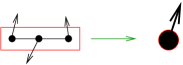
Figure 12: QRG renormalization of $H_{B}$.

The RG-truncation is implemented by means of a truncation operator $O$ constructed from the lowest energy eigenvalues of $H_{B}$ retained during the renormalization process. In this example, $O$ is constructed from the lowest energy doublet in the Clebsch-Gordan decomposition (52), namely (53). Similarly, in the distillation process we have that the tensor product of Alice and Bob’s states can be decomposed into states with coincident qubits in the target, denoted by $\rho^{a}_{\rm C}$ (4), and states with non-coincident qubits in the target, denoted by $\rho^{a}_{\rm NC}$ (4), i.e.,

$$\rho_{AB}\otimes\rho_{AB}=(\sum_{a}\rho^{a}_{\rm C})\oplus(\sum_{a}\rho^{a}_{\rm NC}),$$ (54)

where the sum in $a$ runs over a certain number of mixed states of 4 parties. Notice that this stage is similar to the RG-stage represented by equation (52). Next, an elimination process similar to the RG-truncation is performed by means of LOCC operations (measurements and classical communication) that retains only the bipartite states embedded in the $\rho^{a}_{\rm C}$ states.

Then, the renormalization of the block Hamiltonian is simply

$${H_{B^{\prime}}}={O}{H_{B}}{O^{\dagger}}=E_{0}=-{J}.$$ (55)

Similarly, we could have expressed the state-elimination of the distillation in previous sections in terms of an truncation operator, say $O_{D}$, such that the new mixed state $\rho^{\prime}_{AB}$ is obtained as

$${\rho^{\prime}_{AB}}={O_{D}}(\rho_{AB}\otimes\rho_{AB}){O^{\dagger}_{D}}.$$ (56)

In the case of the quantum Hamiltonian, we still need extra work since there are interaction links between blocks (see Fig. 9). These are absent in the distillation protocol. However, the renormalization of the interblock Hamiltonian $H_{BB}$ follows also the same prescription as in (55) and we arrive at

$${J}{\bf{S}}_{r}^{n}\cdot{\bf{S}}_{l}^{n+1}\xrightarrow{\rm{RG}}{J}(\frac{2}{3})^{2}{\bf{S}}^{\prime}_{n}\cdot{\bf{S}}^{\prime}_{n+1},$$ (57)

where we denote by $n$ and $n+1$ two successive blocks in the original lattice (see Fig. 13) that become two successive sites (see Fig. 12) in the new lattice after the renormalization. We can collect all these steps in Table 3 white , jaitisi . This table should be contrasted with the similar table for the distillation process that can be formed with the steps explained in Sect. II.

1/ Block Decomposition: $H=H_{B}+H_{BB}$.
2/ Diagonalization of $H_{B}$.
3/ Truncation within each Block: $O$.
4/ Renormalization: $H^{\prime}_{B}=OH_{B}O^{\dagger}$, $H^{\prime}_{BB}=OH_{BB}O^{\dagger}$
5/ Iteration: Go to 1/ with $H^{\prime}=H^{\prime}_{B}+H^{\prime}_{BB}$.

Table 3: Steps of the quantum renormalization group method (QRG) for lattice Hamiltonians.

The outcome of the RG-method is that we obtain the correct RG-flow for the coupling constant $J\longrightarrow 0$, signalling a gapless system plus an approximate estimation for the ground state energy, which by means of the variational principle, it is an upper bound for the exact energy. Therefore, the QRG is an energy minimization procedure. Likewise, the purification process produces a protocol for fidelity maximization along with a distillation-flow diagram.

\psfrag{c}[Bc][Bc][1][0]{${\bf{S}}_{r}$}\psfrag{d}[Bc][Bc][1][0]{${\bf{S}}_{l}$}\psfrag{r}[Bc][Bc][0.75][0]{r}\psfrag{l}[Bc][Bc][0.75][0]{l}\psfrag{a}[Bc][Bc][1][0]{$n$}\psfrag{b}[Bc][Bc][1][0]{$n+1$}\includegraphics[scale={0.45}]{chainrlblocks}

Figure 13: QRG renormalization of the interblock Hamiltonian $H_{BB}$.

This completes the relationship established in Table 2 between quantum distillation and quantum renormalization.

VII Conclusions

The field of quantum distillation protocols has become very active in the theory of quantum information due to the central role played by entanglement in the quantum communication procedures and its tendency to degradation.

In this work we have been interested in several extensions of the purification protocols when dealing with multilevel systems (qudits) instead of the more usual qubit protocols. We have seen the various advantages of having distillation methods for qudits systems as compared with the simple case of qubits. We have also obtained the general form of the solution to the distillation recursion relations and several particular solutions have been studied explicitly. We have developed the relationship between quantum distillation protocols and quantum renormalization group methods, something which is interesting in itself and could serve as a guide for possible extension of purification methods.

We would like to mention that the possibility of working with qudits systems has become quite realistic in the recent years. For instance, it is possible to realize multilevel systems in terms of the orbital angular momentum of photons, instead of the more standard polarization (qubit) degree of freedom zeilinger2 , arnaut , barnett . Yet another possibility is to use the so called multiport beam splitters reck , zukowski , molina-terriza , padgett .

There are several ways in which this work can be extended. One is the consideration of noise as as source of errors during the distillation protocol itself. Another one is to allow the possibility of having these distillation protocols for qudits be embedded into a quantum repeater protocol repeaters-pur , repeaters-com .

Acknowledgments. This work is partially supported by the DGES under contract BFM2000-1320-C02-01.

Appendix A General Solution of the Distillation Recursion Relations

In this appendix, we look for more general solutions to the general distillation recursion relations (23) than those studied in section III. To this end, it is convenient to introduce auxiliary variables $g_{kj}^{(n)}$ defined by

$$g_{kj}^{(n)}=\sum_{k^{\prime}=0}^{D-1}g_{k\ominus k^{\prime}j}^{(n-1)}g_{k^{\prime}j}^{(n-1)},\ g_{kj}^{(0)}=q_{kj}^{(0)},$$ (58)

so that the real weights $q_{kj}^{(n)}$ are related to these auxiliary variables as

$$q_{kj}^{(n)}:=\frac{g_{kj}^{(n)}}{\sum_{l,i=0}^{D-1}g_{li}^{(n)}}.$$ (59)

Thus, $g_{kj}^{(n)}$ are unnormalized probability weights. The recursion relations they satisfy can be read as follows (58): for a fixed second index $j$, the unnormalized weights $g_{kj}^{(n)}$ at the step $n$ of the distillation process are obtained as the convolution over the first indices $k$ of the unnormalized weights $g_{kj}^{(n-1)}$ in an earlier step. This fact calls for the introduction of the Fourier transform in order to analyze the relations (58). Let us introduce the new variables $R_{j}^{(n)}$ defined as

$$R_{\hat{k}j}^{(n)}:=\sum_{k=0}^{D-1}\mathord{\rm e}^{\frac{2\pi\mathord{\rm i}\hat{k}k}{D}}g_{kj}^{(n)}.$$ (60)

Now, using the properties of the convolution and the Fourier transform it is inmediate to arrive at a simpler recursion relation

$$R_{\hat{k}j}^{(n)}=\left[R_{\hat{k}j}^{(n-1)}\right]^{2},$$ (61)

which can be iterated all the way down to the initial step

$$R_{\hat{k}j}^{(n)}=\left[R_{\hat{k}j}^{(0)}\right]^{(2^{n})}.$$ (62)

Fourier transforming back to the unnormalized variables, we get

$$g_{kj}^{(n)}=\frac{1}{D}\sum_{\hat{k}=0}^{D-1}\mathord{\rm e}^{-\frac{2\pi\mathord{\rm i}k\hat{k}}{D}}\left[\sum_{k^{\prime}=0}^{D-1}\mathord{\rm e}^{\frac{2\pi\mathord{\rm i}\hat{k}k^{\prime}}{D}}q_{k^{\prime}j}^{(0)}\right]^{(2^{n})},$$ (63)

from which we also obtain the normalized probability weights $q_{kj}^{(n)}$ upon normalization (59). In particular, for the case of qubits treated in Sect. II, $D=2$ and if we also restrict ourselves to weights of the form $q_{00}=F,q_{01}=1-F,q_{10}=q_{11}=0$, we again obtain from the general solution (63) the simple recursion relation in equation (7).

References

- (1) M. Lewenstein, D. Bruss, J.I. Cirac, B. Kraus, M. Kus, J. Samsonowicz, A. Sanpera, R. Tarrach, “Separability and distillability in composite quantum systems -a primer-”, J. Mod. Opt. 47, 2841 (2000).
- (2) D. Bruss, J.I. Cirac, P. Horodecki, F. Hulpke, B. Kraus, M. Lewenstein, A. Sanpera, “Reflections upon separability and distillability”, J. Mod. Opt. 49, 1399-1418 (2002).
- (3) C.H. Bennett, G. Brassard, S. Popescu, B. Schumacher, J.A. Smolin, W.K. Wootters, “Purification of Noisy Entanglement and Faithful Teleportation via Noisy Channels”, Phys. Rev. Lett. 76, 722-725 (1996).
- (4) J.W. Pan, C. Simon, C. Brukner, A. Zeilinger, “Feasible Entanglement Purification for Quantum Communication”, Nature 410, 1067 (2001).
- (5) N. Gisin, “Hidden quantum nonlocality revealed by local filters”, Phys. Lett. A210, 151, (1996).
- (6) P.G. Kwiat, S. Barraza-Lopez, A. Stefanov, N. Gisin, “Experimental entanglement distillation and ’hidden’ non-locality,” Nature 409, 1014 (2001).
- (7) P.W. Shor, “Scheme for reducing decoherence in quantum computer memory”, Phys. Rev. A52, 2493-2496, (1995).
- (8) A.M. Steane, “Error correcting codes in quantum theory”, Phys. Rev. Lett. 77, 793, (1996).
- (9) D. Gottesman, “A theory of fault-tolerant quantum computation,” Phys. Rev. A 57, 127-137 (1998).
- (10) J. Preskill, “Fault-tolerant quantum computation.” quant-ph/9712048.
- (11) C.H. Bennett, D.P. DiVincenzo, J. Smolin, W.K. Wooters, “Mixed-state entanglement and quantum error correction”, Phys. Rev. A54, 3824 (1996).
- (12) D. Deutsch, A. Ekert, R. Jozsa, C. Macchiavello, S. Popescu, A. Sanpera, “Quantum Privacy Amplification and the Security of Quantum Cryptography over Noisy Channels”, Phys. Rev. Lett. 77, 2818-2821 (1996).
- (13) C. Macchiavello, “On the analytical convergence of the QPA procedure”, Phys. Lett. A246, 385 (1998).
- (14) C. Macchiavello, “Quantum Privacy Amplification”, in D. Bouwmeester, A. Ekert, A. Zeilinger (eds.), The physics of quantum information, Springer-Verlag 2000.
- (15) W. Dür, H.-J. Briegel, J.I. Cirac, P. Zoller, “Quantum repeaters based on entanglement purification”, Phys. Rev. A. 59, 169 (1999).
- (16) W. Dür, H.-J. Briegel, J.I. Cirac, P. Zoller, “Quantum repeaters for communication”, quant-ph/9803056.
- (17) M. Horodecki, P. Horodecki, “Reduction criterion of separability and limits for a class of distillation protocols”, Phys. Rev. A59, 4206-4216, (1999).
- (18) G. Alber, A. Delgado, N. Gisin, I. Jex, “Generalized quantum XOR-gate for quantum teleportation and state purificationin arbitrary dimensional Hilbert spaces”, quant-ph/000802.
- (19) G. Alber, A. Delgado, N. Gisin, I. Jex, “Efficient bipartite quantum state purification in arbitrary dimensional Hilbert spaces”, quant-ph/0102035.
- (20) H. Bechmann-Pasquinucci, A. Peres, “Quantum Cryptography with 3-State Systems”, Phys. Rev. Lett. 85, 3313-3316, (2000).
- (21) H. Bechmann-Pasquinucci, W. Tittel, “Quantum cryptography using larger alphabets”, Phys. Rev. A 61, 062308 (2000).
- (22) M. Bourennane, A. Karlsson, G. Björk, “Quantum key distribution using multilevel encoding”, Phys. Rev. A 64, 012306 (2001).
- (23) C.H. Bennett, H.J. Berstein, S. Popescu, B. Schumacher, “Concentrating partial entanglement by local operations”, Phys. Rev. A53, 2046 (1996).
- (24) J. González, M.A. Martín-Delgado, G. Sierra, A.H. Vozmediano, Quantum Electron Liquids and High- Superconductivity, Lecture Notes in Physics, Monographs vol. 38. Springer-Verlag 1995.
- (25) M.A. Martín-Delgado, G. Sierra; “Analytic Formulations of the Density Matrix Renormalization Group”; Int. J. Mod. Phys. A11, 3147-3174 (1996).
- (26) S.R. White, “Density-matrix algorithms for quantum renormalization groups” Phys. Rev. B48, 10345 (1993).
- (27) A. Mair, A. Vaziri, G. Weihs, A. Zeilinger, “Entanglement of Orbital Angular Momentum States of Photons”, Nature 412, 3123-316 (2001).
- (28) H.H. Arnaut, G.A. Barbosa, “Orbital and Intrinsic Angular Momentum of Single Photons and Entangled Pairs of Photons Generated by Parametric Down-Conversion” Phys. Rev. Lett. 85, 286 (2000).
- (29) S. Franke-Arnold, S.M. Barnett, “Two-photon entanglement of orbital angular momentum states”, Phys. Rev. A65, 033823 (2002).
- (30) M. Reck, A. Zeilinger, H.J. Bernstein, P. Bertani, “Experimental realization of any discrete unitary operator”, Phys. Rev. Lett. 73, 58-61 (1994).
- (31) M. Zukowski, A. Zeilinger, M.A. Horne, “Realizable higher-dimensional two-particle entanglements via multiport beam splitters”, Phys. Rev. A 55, 2564-2579 (1997).
- (32) G. Molina-Terriza, J.P. Torres, L. Torner, “Management of the Angular Momentum of Light: Preparation of Photons in Multidimensional Vector States of Angular Momentum”, Phys. Rev. Lett. 88, 013601 (2002).
- (33) J. Leach, M.J. Padgett, S.M. Barnett, S. Franke-Arnold, J. Courtial, “Measuring the Orbital Angular Momentum of a Single Photon”, Phys. Rev. Lett. 88, 257901 (2002).