Unitary time-dependent superconvergent technique for pulse-driven quantum dynamics

Abstract

We present a superconvergent Kolmogorov-Arnold-Moser type of perturbation theory for time-dependent Hamiltonians. It is strictly unitary upon truncation at an arbitrary order and not restricted to periodic or quasiperiodic Hamiltonians. Moreover, for pulse-driven systems we construct explicitly the KAM transformations involved in the iterative procedure. The technique is illustrated on a two-level model perturbed by a pulsed interaction for which we obtain convergence all the way from the sudden regime to the opposite adiabatic regime.

I Introduction

The control of atomic and molecular dynamics by lasers has attracted considerable interest in the past decade. Time-dependent systems are traditionally studied from a perturbative point of view with the Dyson expansion. The two limiting cases of a sudden and an adiabatic switching of the perturbation have been extensively studied [1]. In particular, this has resulted in the adiabatic theorem and the superadiabatic expansion [2, 3].

We are interested in the case where the perturbation is switched on and off on a time scale which need not be arbitrarily small or large. It is well known that generally, upon truncation, the Dyson series for the evolution operator of a non-autonomous system is not unitary, giving rise to secular terms whose size grows with time. For periodic and quasi-periodic perturbations, a number of schemes have been proposed [4], notably one based on the Kolmogorov-Arnold-Moser (KAM) perturbation theory of classical mechanics [5]. Here we shall not be dealing with periodic or quasiperiodic systems but with time-dependent perturbations that are localized in time for which we develop, building on the KAM technique, a unitary superconvergent perturbation theory.

The KAM iterative method has been introduced in quantum mechanics by Belissard [6] for periodic Hamiltonians. It consists in generating at each step (with the help of a unitary transformation) a new reference or effective Hamiltonian which collects higher order terms of the perturbation that commute with the reference Hamiltonian constructed at the preceding step. At the first iteration the order of the perturbation is reduced from $\epsilon$ to $\epsilon^{2}$ and, by considering the resulting Hamiltonian as a new starting point, the second transformation then reduces the order of the perturbation from $\epsilon^{2}$ to $\epsilon^{4}$. Hence, at the $n$-th iteration the size of the remaining perturbation is reduced from $\epsilon^{2^{n-1}}$ to $\epsilon^{2^{n}}$. The quantum KAM technique has also been investigated for periodic Hamiltonians by Combescure [7, 8] and more recently by Duclos and  Šťovícek [9]. Quasiperiodic Hamiltonians have been considered by Blekher et al. in [10].

All these authors have implemented the KAM algorithm in an extended Hilbert space constructed as the tensor product of the Hilbert space in which the original Hamiltonian is defined and the space of square integrable functions on the circle. This notion, introduced by Sambe [11] in the periodic case and by Howland [12] for more general time-dependent Hamiltonians, allows to construct a time-independent extended Hamiltonian (also called Floquet Hamiltonian in the periodic case) which is the starting point in the KAM algorithm.

The KAM iterative procedure requires solving two commutator equations at each step. In [13, 14] Scherer has shown, adapting ideas from classical mechanics going back to Poincaré, that these equations could be solved in terms of time averages of some operators related to the perturbation.

The generalisation of the KAM technique to time-dependent Hamiltonians has been worked out by Scherer [15, 16]. It has been built in close analogy to classical mechanics and involves an extended phase space which includes time as a coordinate and the energy of external sources as its conjugate momentum, a notion closely related to that of [12]. On the other hand, the KAM algorithm proposed by Scherer is quite cumbersome to use and, in addition, is not guaranteed to yield a unitary evolution operator upon truncation.

In this paper we present a KAM algorithm for non-autonomous Hamiltonians that is strictly unitary upon truncation at an arbitrary order. Moreover, for pulse-driven systems we construct explicitly the KAM transformations and study the convergence of the algorithm on a specific case.

We start in Sec. II.1 by recalling the KAM technique and the quantum averaging method for time-independent Hamiltonians. The notion of extended Hilbert space is presented in Sec. II.2 at a purely formal level. In Sec. II.3 we construct a unitary KAM algorithm for time-dependent systems in an extended Hilbert space. In Sec. II.4 the quantum averaging technique is extended to non-autonomous Hamiltonians in order to construct the KAM transformations directly in the original Hilbert space. Sec. III.1 is devoted to perturbations that are switched on at some finite time in the past, for which we calculate explicitly the successive time averages involved in the KAM algorithm. We then focus on the case of pulse-driven two-levels systems, for which we resum exactly in Sec. III.2 the infinite series of commutators yielding the remaining perturbations at a given step of the iterative procedure. Finally, in Sec. III.3 the method is applied to a two-level system interacting with a sine-squared pulse, taking the ratio of the characteristic duration of the pulse and the characteristic time of the free evolution as the small parameter $\epsilon$. We show the remarkable result that the KAM algorithm converges for all values of the parameter $\epsilon$, even larger than unity, allowing to go from the sudden regime to the opposite adiabatic regime. The conclusions are given in Sec. IV while some details of the calculations are reported in Appendices A and B.

II Unitary superconvergent time-dependent perturbation theory

II.1 KAM algorithm for autonomous Hamiltonians

In this section, we present the KAM technique for a time-independent Hamiltonian following the formulation of [6] and using the averaging method of [14]. Let $K_{1}=K_{0}+\epsilon V_{1}$ where $K_{0}$ is a reference Hamiltonian defined on a Hilbert space $\mathbb{H}$ and $\epsilon V_{1}$ a bounded self-adjoint perturbation with small parameter $\epsilon$. As will become clear below, the subscript $n$ indicates that an operator $A_{n}$ is involved in the $n$-th iteration. On the other hand, the upperscript e stands for effective and indicates that an operator $B^{{\rm e}}_{n}$ constructed at the $n$-th step will be taken as the new reference at the next step. Throughout the paper the leading order in $\epsilon$ will appear explicitly in front of the operators which are thus themselves of order $\epsilon^{0}$ but may still depend on $\epsilon$ although we shall not indicate it explicitly. We look for the generator $W_{1}$ of a unitary transform $T_{1}\equiv e^{\epsilon W_{1}}$ such that

$$T_{1}^{\dagger}K_{1}T_{1}\equiv T_{1}^{\dagger}(K_{0}+\epsilon V_{1})T_{1}=K^{{\rm e}}_{1}+\epsilon^{2}V_{2}\equiv K_{2}\,,$$ (1)

with $[K^{{\rm e}}_{1},K_{0}]=0$. Writing $K^{{\rm e}}_{1}\equiv K_{0}+\epsilon D_{1}$, the unknown $W_{1}$ and $D_{1}$ are solutions of the following commutator equations:

$$\left[K_{0},D_{1}\right]=0\,,$$ (2a)

$$\left[K_{0},W_{1}\right]+V_{1}=D_{1}\,.$$ (2b)

The remainder $\epsilon^{2}V_{2}$ contains all the terms of Eq. (1) which are not of order $\epsilon^{0}$ (which disappear trivially) or of order $\epsilon$ (which disappear identically because of Eq. (2b)). It reads

$$\epsilon^{2}V_{2} = -\frac{\epsilon^{2}}{2}\left[W_{1},V_{1}\right]-\frac{\epsilon^{2}}{2}\left[W_{1},D_{1}\right]$$ (3)

$$+ \frac{\epsilon^{3}}{3}\left[W_{1},\left[W_{1},V_{1}\right]\right]+\frac{\epsilon^{3}}{6}\left[W_{1},\left[W_{1},D_{1}\right]\right]+\ldots,\quad$$

or, writing the series of commutator in a compact form that we shall use later,

$$\epsilon^{2}V_{2}=\sum_{k=1}^{\infty}\frac{(-1)^{k}\epsilon^{k+1}}{(k+1)!}\,\left\{k\,{\rm ad}^{k}(W_{1},V_{1})+{\rm ad}^{k}(W_{1},D_{1})\right\},\$$ (4)

where

$${\rm ad}^{k}(A,B)\equiv\left\{\begin{array}[]{ll}B&k=0\\ \left[A,{\rm ad}^{k-1}(A,B)\right]&k\geq 1.\end{array}\right.$$ (7)

The solutions to Eqs. (2) can be written in terms of averages:

$$D_{1}\!\! = \!\!\lim_{T\rightarrow\infty}\frac{1}{T}\int_{0}^{T}e^{-itK_{0}}V_{1}e^{itK_{0}}\mathrm{d}t\ \equiv\ \overline{V_{1}}^{K_{0}},$$ (8a)

$$W_{1}\!\! = \!\!\lim_{T\rightarrow\infty}\frac{-i}{T}\int_{0}^{T}\!\mathrm{d}t\!\int_{0}^{t}\mathrm{d}t^{\prime}e^{-it^{\prime}K_{0}}\left(V_{1}-\overline{V_{1}}^{K_{0}}\right)e^{it^{\prime}K_{0}}$$ (8b)

$$\equiv -i\widehat{V_{1}}^{K_{0}}.$$

This is readily checked upon substitution, noting that $e^{-itK_{0}}$ is the propagator of the reference Hamiltonian $K_{0}$ in units such that $\hbar$=1. The shorthand notations on the right handside of Eqs. (8) can be viewed as well defined linear transformations of the operator $V_{1}$.

The process can be iterated, transforming now the operator $K_{2}$ defined by Eq. (1) with $T_{2}=e^{\epsilon^{2}W_{2}}$ and considering $K^{{\rm e}}_{1}$ as the new reference operator:

$$T_{2}^{\dagger}K_{2}T_{2}\equiv T_{2}^{\dagger}(K^{{\rm e}}_{1}+\epsilon^{2}V_{2})T_{2}=K^{{\rm e}}_{2}+\epsilon^{4}V_{3}\equiv K_{3}\,,$$ (9)

with $[K^{{\rm e}}_{2},K^{{\rm e}}_{1}]=0$. Notice that the new perturbation is not of order $\epsilon^{3}$ as would be the case in a standard perturbation theory, but of order $\epsilon^{4}$. Similarly, after $n$ iterations we obtain

$$T_{n}^{\dagger}K_{n}T_{n}=K^{{\rm e}}_{n}+\epsilon^{2^{n}}V_{n+1}\equiv K_{n+1}\,,$$ (10)

with $[K^{{\rm e}}_{n},K^{{\rm e}}_{n-1}]=0$. The new reference Hamiltonian $K^{{\rm e}}_{n}$ is written

$$K^{{\rm e}}_{n}=K^{{\rm e}}_{n-1}+\epsilon^{2^{n-1}}D_{n}=K_{0}+\sum_{j=1}^{n}\epsilon^{2^{j-1}}D_{j}\,.$$ (11)

The generator $W_{n}$ of the unitary transformation $T_{n}=e^{\epsilon^{2^{n-1}}W_{n}}$ and the operator $D_{n}$, solving equations analogous to Eqs. (2), are calculated as

$$D_{n} = \overline{V_{n}}^{K^{{\rm e}}_{n-1}}\,,$$ (12a)

$$W_{n} = -i\widehat{V_{n}}^{K^{{\rm e}}_{n-1}}\,.$$ (12b)

The remainder being of order $\epsilon^{2^{n}}$, the KAM algorithm is called superconvergent. However, we emphasize that a proof of convergence is to be established in each case. We also note that in the absence of resonances, $\epsilon$ need not be small for this algorithm to converge [17].

II.2 Extended Hilbert space

Given a time-dependent Hamiltonian $H(t)$ acting on a Hilbert space $\mathbb{H}$, we recall here how the notion of extended Hilbert space of [12] allows to construct a time-independent operator on that space. Let $U_{H}(t,t_{0})$ denote the evolution operator associated to $H(t)$, so that the Schrödinger equation and the initial condition read

$$i\frac{\partial}{\partial t}U_{H}(t,t_{0})=H(t)U_{H}(t,t_{0})\ ,\quad U_{H}(t_{0},t_{0})=\openone_{\mathbb{H}}\,,$$ (13)

where $\openone_{\mathbb{H}}$ is the identity operator on $\mathbb{H}$. We introduce a parameter $s\in\mathbb{R}$ which plays the role of an arbitrary reference time, and let $U_{H}(t,t_{0};s)$ be the solution of Eqs. (13) now with $H(t+s)$. In $\mathbb{H}$, the operator $U_{H}(t,t_{0};s)$ depends parametrically on $s$. Notice that $U_{H}(t,t_{0};0)=U_{H}(t,t_{0})$.

An extended Hilbert space $\mathbb{K}$ where $s$ is now an additional coordinate can be defined as the tensor product of $\mathbb{L}$ and $\mathbb{H}$ where $\mathbb{L}\equiv\mathcal{L}_{2}(\mathbb{R})$ is the space of square integrable functions on the real line: $\mathbb{K}\equiv\mathbb{L}\otimes\mathbb{H}$. The family of operators $U_{H}(t,t_{0};s)$ acting on $\mathbb{H}$ is lifted to the operator $\mathcal{U}_{\mathcal{H}}(t,t_{0};s)$ defined on $\mathbb{K}$ by considering the full dependence on $s$ as a multiplication operator on $\mathbb{L}$. Similarly, the family of operators $H(t+s)$ on $\mathbb{H}$ is lifted to the operator $\mathcal{H}(t+s)$ on $\mathbb{K}$. We shall denote operators acting on the extended Hilbert space $\mathbb{K}$ by uppercase calligraphic letters and shall refer to $\mathcal{U}_{\mathcal{H}}(t,t_{0};s)$ and $\mathcal{H}(t+s)$ as the lifts of $U_{H}(t,t_{0})$ and $H(t)$ respectively (with the understanding that the family of operators $U_{H}(t,t_{0};s)$ or $H(t+s)$ is considered as an intermediate step). The lift of Eqs. (13) on the extended Hilbert space $\mathbb{K}$ reads

$$i\frac{\partial}{\partial t}\mathcal{U}_{\mathcal{H}}(t,t_{0};s)={\mathcal{H}}(t+s)\mathcal{U}_{\mathcal{H}}(t,t_{0};s)\,,$$ (14a)

$$\mathcal{U}_{\mathcal{H}}(t_{0},t_{0};s)={\openone}_{\mathbb{L}}\otimes{\openone}_{\mathbb{H}}\,.$$ (14b)

where ${\openone}_{\mathbb{L}}$ is the identity operator on $\mathbb{L}$. Notice that

$$\mathcal{U}_{\mathcal{H}}(t+s^{\prime},t_{0}+s^{\prime};s-s^{\prime})=\mathcal{U}_{\mathcal{H}}(t,t_{0};s)\quad\forall s^{\prime}\in\mathbb{R}.$$ (15)

Finally, an extended Hamiltonian is defined on $\mathbb{K}$ as the time-independent self-adjoint operator ${\mathcal{K}}\equiv{\mathcal{H}}(s)-i\frac{\partial}{\partial s}\otimes\openone_{\mathbb{H}}$. Its associated unitary evolution operator reads $\mathcal{U}_{\mathcal{K}}(t,t_{0})\equiv e^{-i(t-t_{0}){\mathcal{K}}}$ and is related to the solution of Eqs. (14) by the following equation which is easily derived:

$$\mathcal{U}_{\mathcal{K}}(t,t_{0})={\sf T}_{-t}\mathcal{U}_{\mathcal{H}}(t,t_{0};s){\sf T}_{t_{0}}\,,$$ (16)

where the translation operator ${\sf T}_{t}$ acts on functions $\xi(s)\in\mathbb{L}$ according to ${\sf T}_{t}\xi(s)=\xi(s+t)$ and can be expressed as ${\sf T}_{t}=e^{t\frac{\partial}{\partial s}}$.

II.3 KAM algorithm in the extended Hilbert space for non-autonomous Hamiltonians

We consider $\epsilon V_{1}(t)$ as a bounded time-dependent perturbation of the time-dependent reference Hamiltonian $H_{0}(t)$ defined on the Hilbert space $\mathbb{H}$ and whose propagator $U_{H_{0}}(t,t_{0})$ is known. Our aim is to obtain a KAM expansion for the evolution operator $U_{H_{1}}(t,t_{0})$ of the full Hamiltonian $H_{1}(t)\equiv H_{0}(t)+\epsilon V_{1}(t)$. We first consider the extended Hilbert space $\mathbb{K}=\mathbb{L}\otimes\mathbb{H}$, and the lifts $\mathcal{U}_{\mathcal{H}_{1}}(t,t_{0};s)$ and $\mathcal{H}_{1}(t+s)$ of the operators $U_{H_{1}}(t,t_{0})$ and $H_{1}(t)$ as defined in Sec. II.2. Similarly, $\mathcal{U}_{\mathcal{H}_{0}}(t,t_{0};s)$, $\mathcal{H}_{0}(t+s)$ and $\mathcal{V}_{1}(t+s)$ denote the lifts on $\mathbb{K}$ of $U_{H_{0}}(t,t_{0})$, $H_{0}(t)$ and $V_{1}(t)$. We then define the associated extended Hamiltonian on $\mathbb{K}$:

$$\mathcal{K}_{1}\!\!\! \equiv \!\!\!\mathcal{H}_{1}(s)-i\frac{\partial}{\partial s}\otimes\openone_{\mathbb{H}},$$ (17a)

$$= \!\!\!\mathcal{H}_{0}(s)-i\frac{\partial}{\partial s}\otimes\openone_{\mathbb{H}}+\epsilon\mathcal{V}_{1}(s)\equiv\mathcal{K}_{0}+\epsilon\mathcal{V}_{1}(s),\qquad$$ (17b)

which is of the form considered in Sec. II.1. Hence, we can now apply the KAM technique in the extended Hilbert space to obtain a KAM expansion for the time-independent operator $\mathcal{K}_{1}$.

At the $n$-th iteration of the algorithm, the operator $\mathcal{K}_{n}=\mathcal{K}^{{\rm e}}_{n-1}+\epsilon^{2^{n-1}}\mathcal{V}_{n}(s)$ is transformed by the unitary operator $\mathcal{T}_{n}(s)$ according to

$$\mathcal{T}_{n}^{\dagger}(s)\mathcal{K}_{n}\mathcal{T}_{n}(s)=\mathcal{K}^{{\rm e}}_{n}+\epsilon^{2^{n}}\mathcal{V}_{n+1}(s)\,,\ \$$ (18)

with

$$\mathcal{K}^{{\rm e}}_{n} = \mathcal{H}^{{\rm e}}_{n}(s)-i\frac{\partial}{\partial s}\otimes\openone_{\mathbb{H}},$$ (19a)

$$\mathcal{H}^{{\rm e}}_{n}(s) = \mathcal{H}^{{\rm e}}_{n-1}(s)+\epsilon^{2^{n-1}}\overline{\mathcal{V}_{n}}^{\mathcal{K}^{{\rm e}}_{n-1}}(s),$$ (19b)

$$\mathcal{T}_{n}(s) = \exp\left(-i\epsilon^{2^{n-1}}\widehat{\mathcal{V}_{n}}^{\mathcal{K}^{{\rm e}}_{n-1}}(s)\right).$$ (19c)

The remainder $\epsilon^{2^{n}}\mathcal{V}_{n+1}(s)$ is given by an expression analogous to Eq. (4):

$$\epsilon^{2^{n}}\mathcal{V}_{n+1}(s)=\sum_{k=1}^{\infty}\frac{i^{k}\epsilon^{(k+1)2^{n-1}}}{(k+1)!}\left\{k\,{\rm ad}^{k}\left(\widehat{\mathcal{V}_{n}}^{\mathcal{K}^{{\rm e}}_{n-1}}(s),\mathcal{V}_{n}(s)\right)+{\rm ad}^{k}\left(\widehat{\mathcal{V}_{n}}^{\mathcal{K}^{{\rm e}}_{n-1}}(s),\overline{\mathcal{V}_{n}}^{\mathcal{K}^{{\rm e}}_{n-1}}(s)\right)\right\}.\quad$$ (20)

The operators $\overline{\mathcal{V}_{n}}^{\mathcal{K}^{{\rm e}}_{n-1}}(s)$ and $\widehat{\mathcal{V}_{n}}^{\mathcal{K}^{{\rm e}}_{n-1}}(s)$, defined by Eqs. (8), can be expressed in terms of the operator $\mathcal{U}_{\mathcal{H}^{{\rm e}}_{n-1}}(t,t_{0};s)$ using Eq. (16) for the propagator of $\mathcal{K}^{{\rm e}}_{n}$:

$$\overline{\mathcal{V}_{n}}^{\mathcal{K}^{{\rm e}}_{n-1}}(s)\!\! = \!\!\lim_{T\rightarrow\infty}\frac{1}{T}\int_{0}^{T}\!\mathrm{d}t\,\mathcal{U}_{\mathcal{H}^{{\rm e}}_{n-1}}(0,-t;s)\mathcal{V}_{n}(s-t)\mathcal{U}_{\mathcal{H}^{{\rm e}}_{n-1}}^{\dagger}(0,-t;s)\equiv\overline{\mathcal{V}_{n}}^{\mathcal{H}^{{\rm e}}_{n-1}}(s),$$ (21a)

$$\widehat{\mathcal{V}_{n}}^{\mathcal{K}^{{\rm e}}_{n-1}}(s)\!\! = \!\!\lim_{T\rightarrow\infty}\frac{1}{T}\int_{0}^{T}\!\mathrm{d}t^{\prime}\!\int_{0}^{t^{\prime}}\!\mathrm{d}t\,\mathcal{U}_{\mathcal{H}^{{\rm e}}_{n-1}}(0,-t;s)\left[\mathcal{V}_{n}(s-t)-\overline{\mathcal{V}_{n}}^{\mathcal{K}^{{\rm e}}_{n-1}}(s-t)\right]\mathcal{U}_{\mathcal{H}^{{\rm e}}_{n-1}}^{\dagger}(0,-t;s)\equiv\widehat{\mathcal{V}_{n}}^{\mathcal{H}^{{\rm e}}_{n-1}}(s).\qquad$$ (21b)

On the other hand, from Eqs. (16) and (19) and the fact that $\mathcal{K}^{{\rm e}}_{n}$ commutes with all the operators $\mathcal{K}^{{\rm e}}_{k}$ constructed at the preceding iterations one deduces that

$$\mathcal{U}_{\mathcal{H}^{{\rm e}}_{n}}(t,t_{0};s)\! = \!\mathcal{U}_{\mathcal{H}_{0}}(t,t_{0};s)\,\mathcal{S}_{1}(t,t_{0};s+t_{0})\ldots\mathcal{S}_{n}(t,t_{0};s+t_{0}),\qquad$$ (22a)

$$= \!\mathcal{S}_{1}(t,t_{0};s+t)\ldots\mathcal{S}_{n}(t,t_{0};s+t)\,\mathcal{U}_{\mathcal{H}_{0}}(t,t_{0};s),\qquad$$ (22b)

where $\mathcal{S}_{p}(t,t_{0};s)$ denotes the following operator on $\mathbb{K}$:

$$\mathcal{S}_{p}(t,t_{0};s)\equiv\exp{\left(-i(t-t_{0})\epsilon^{2^{p-1}}\overline{\mathcal{V}_{p}}^{\mathcal{H}^{{\rm e}}_{p-1}}(s)\right)}.$$ (23)

The detailled derivation of Eqs. (21) and (22) is provided in appendix A. It follows that $\overline{\mathcal{V}_{n}}^{\mathcal{H}^{{\rm e}}_{n-1}}(s)$ and $\widehat{\mathcal{V}_{n}}^{\mathcal{H}^{{\rm e}}_{n-1}}(s)$ are calculated from $\mathcal{U}_{\mathcal{H}_{0}}(t,t_{0};s)$ as well as the operators $\overline{\mathcal{V}_{p}}^{\mathcal{H}^{{\rm e}}_{p-1}}(s)$ and $\widehat{\mathcal{V}_{p}}^{\mathcal{H}^{{\rm e}}_{p-1}}(s)$ constructed at the preceding iterations. Hence, the operators $\mathcal{T}_{n}(s)$, $\mathcal{K}^{{\rm e}}_{n}$ and $\mathcal{V}_{n+1}(s)$ entering Eq. (18) are now entirely determined.

The extended Hamiltonian $\mathcal{K}_{1}$ we started with can be expressed in terms of $\mathcal{K}^{{\rm e}}_{n}$ by repeated use of Eq. (18):

$$\mathcal{K}_{1}=\mathcal{T}_{1}(s)\ldots\mathcal{T}_{n}(s)\,\mathcal{K}^{{\rm e}}_{n}\,\mathcal{T}_{n}^{\dagger}(s)\ldots\mathcal{T}_{1}^{\dagger}(s)+\mathcal{O}(\epsilon^{2^{n}}).$$ (24)

The propagator $\mathcal{U}_{\mathcal{K}_{1}}(t,t_{0})=e^{-i(t-t_{0})\mathcal{K}_{1}}$ allows then to construct the operator $\mathcal{U}_{\mathcal{H}_{1}}(t,t_{0};s)$ on $\mathbb{K}$ from Eq. (16). Taking also Eq. (22a) into account yields

$$\mathcal{U}_{\mathcal{H}_{1}}(t,t_{0};s)=\!\!\! \!\!\!\mathcal{T}_{1}(t+s)\ldots\mathcal{T}_{n}(t+s)\,\mathcal{U}_{\mathcal{H}_{0}}(t,t_{0};s)$$ (25)

$$\!\!\!\mathcal{S}_{1}(t,t_{0};s+t_{0})\ldots\mathcal{S}_{n}(t,t_{0};s+t_{0})$$

$$\!\!\!\mathcal{T}_{n}^{\dagger}(t_{0}+s)\ldots\mathcal{T}_{1}^{\dagger}(t_{0}+s)+\mathcal{O}(\epsilon^{2^{n}}).\quad$$

It is now possible to return to the original Hilbert space $\mathbb{H}$, by considering the dependence on the $s-$variable of each of the operators entering Eq. (25), which defines a multiplication operator on $\mathbb{L}$, as a parametric dependence on time in $\mathbb{H}$, and subsequently setting $s=0$. Hence, in agreement with our notations, Eq. (25) is the lift on $\mathbb{K}$ of the following expression for the propagator $U_{H_{1}}(t,t_{0})$ on $\mathbb{H}$:

$$U_{H_{1}}(t,t_{0})=\!\!\! \!\!\!T_{1}(t)\ldots T_{n}(t)\,U_{H_{0}}(t,t_{0})S_{1}(t,t_{0};t_{0})\ldots$$ (26)

$$\!\!\!S_{n}(t,t_{0};t_{0})\,T_{n}^{\dagger}(t_{0})\ldots T_{1}^{\dagger}(t_{0})+\mathcal{O}(\epsilon^{2^{n}}),\qquad$$

where $S_{p}(t,t_{0};t_{0})$ and $T_{p}(t)$ acting on $\mathbb{H}$ are obtained, as just described, from their lift $\mathcal{S}_{p}(t,t_{0};s+t_{0})$ and $\mathcal{T}_{p}(t+s)$ constructed on $\mathbb{K}$.

In practice, however, we shall find it simpler to construct $S_{p}(t,t_{0};t_{0})$ and $T_{p}(t)$ directly in $\mathbb{H}$. As we show below, this can be achieved by considering Eqs. (19b)-(23) which have well defined meaning on $\mathbb{K}$ as the lift of equations for corresponding operators defined on $\mathbb{H}$. In particular, Eq. (21a) with $n=1$ is the lift of a similar equation defining the operator $\overline{V_{1}}^{H_{0}}(t)$ on $\mathbb{H}$ in terms of $U_{H_{0}}(t,t_{0})$ and $V_{1}(t)$.

II.4 KAM expansion in the original Hilbert space for non-autonomous evolution operators

In this section, we shall construct the propagator $U_{H_{1}}(t,t_{0})$ from Eq. (26) through an iterative procedure entirely defined in the Hilbert space $\mathbb{H}$ of the Hamiltonian $H_{1}(t)=H_{0}(t)+\epsilon V_{1}(t)$, i.e. we shall not have to define operators in an extended Hilbert space. The operators $U_{H_{0}}(t,t_{0})$ and $V_{1}(t)$ allow to construct the operator $\overline{V_{1}}^{H_{0}}(t)$ on $\mathbb{H}$ according to Eq. (28a) given below, where we set $p=1$. Subsequently, the operator $\widehat{V_{1}}^{H_{0}}(t)$ can be obtained from these operators using Eq. (28b) with $p=1$. Hence, by Eqs. (27), the operators $S_{1}(t,t_{0};t_{0})$ and $T_{1}(t)$ are determined.

On the other hand, Eq. (28c) with $p=1$ enables us to derive the operator $V_{2}(t)$ on $\mathbb{H}$ from the operators $\overline{V_{1}}^{H_{0}}(t)$ and $\widehat{V_{1}}^{H_{0}}(t)$ we have just constructed. Similarly, Eq. (29) yields the propagator $U_{H^{{\rm e}}_{1}}(t,t_{0})$. It follows that the operators $\overline{V_{2}}^{H^{{\rm e}}_{1}}(t)$ and $\widehat{V_{2}}^{H^{{\rm e}}_{1}}(t)$ can be obtained from Eqs. (28a) and (28b) now with $p=2$.

For $p\geq 1$ we have the following operators on $\mathbb{H}$:

$$S_{p}(t,t_{0};t_{1})\!\! = \!\!\exp{\left(-i(t-t_{0})\epsilon^{2^{p-1}}\overline{V_{p}}^{H^{{\rm e}}_{p-1}}(t_{1})\right)},\qquad$$ (27a)

$$T_{p}(t)\!\! = \!\!\exp{\left(-i\epsilon^{2^{p-1}}\widehat{V_{p}}^{H^{{\rm e}}_{p-1}}(t)\right)},\qquad$$ (27b)

where

$$\overline{V_{p}}^{H^{{\rm e}}_{p-1}}(t)\!\! = \!\!\lim_{T\rightarrow\infty}\frac{1}{T}\int_{t-T}^{t}\!\mathrm{d}u\,U_{H^{{\rm e}}_{p-1}}(t,u)V_{p}(u)U_{H^{{\rm e}}_{p-1}}^{\dagger}(t,u),\quad$$ (28a)

$$\widehat{V_{p}}^{H^{{\rm e}}_{p-1}}(t)\!\! = \!\!\lim_{T\rightarrow\infty}\frac{1}{T}\int_{0}^{T}\!\mathrm{d}t^{\prime}\!\int_{t-t^{\prime}}^{t}\!\mathrm{d}u\,U_{H^{{\rm e}}_{p-1}}(t,u)\left[V_{p}(u)-\overline{V_{p}}^{H^{{\rm e}}_{p-1}}(u)\right]U_{H^{{\rm e}}_{p-1}}^{\dagger}(t,u),$$ (28b)

$$V_{p+1}(t)\!\! = \!\!\sum_{k=1}^{\infty}\frac{i^{k}\epsilon^{(k-1)2^{p-1}}}{(k+1)!}\,\left\{k\,{\rm ad}^{k}\left(\widehat{V_{p}}^{H^{{\rm e}}_{p-1}}(t),V_{p}(t)\right)+{\rm ad}^{k}\left(\widehat{V_{p}}^{H^{{\rm e}}_{p-1}}(t),\overline{V_{p}}^{H^{{\rm e}}_{p-1}}(t)\right)\right\},\quad$$ (28c)

and

$$U_{H^{{\rm e}}_{p}}(t,t_{0})\! = \!U_{H_{0}}(t,t_{0})\,S_{1}(t,t_{0};t_{0})\ldots S_{p}(t,t_{0};t_{0}).\qquad$$ (29)

Note that $H^{{\rm e}}_{p}(t)=H^{{\rm e}}_{p-1}(t)+\epsilon^{2^{p-1}}\overline{V_{p}}^{H^{{\rm e}}_{p-1}}(t)$. By the iterative procedure described here and which rests solely on Eqs. (27)-(29), the operators $S_{p}(t,t_{0};t_{0})$ and $T_{p}(t)$ are constructed entirely in the Hilbert space $\mathbb{H}$. The propagator $U_{H_{1}}(t,t_{0})$ of the non-autonomous Hamiltonian $H_{1}(t)=H_{0}(t)+\epsilon V_{1}(t)$ is then obtained by Eq. (26) up to a desired order in $\epsilon$.

III Pulse-driven systems

III.1 General case

In this section, we consider the physically relevant case of time-dependent perturbations $\epsilon V_{1}(t)$ which are switched on at a given finite time $t_{{\rm i}}$. To allow for some flexibility in the choice of the reference operators we shall consider the slightly more general case of perturbations $\epsilon V_{1}(t)$ which before $t_{{\rm i}}$ are constant in time and commute with the reference propagator $U_{H_{0}}(t,t_{0})$ on $\mathbb{H}$:

$$V_{1}(t)=V_{1}(t_{{\rm i}})\quad\forall t\leq t_{{\rm i}},$$ (30a)

$$\left[V_{1}(t_{{\rm i}}),U_{H_{0}}(t^{\prime},t)\right]=0\quad\forall t,t^{\prime}\leq t_{{\rm i}}.$$ (30b)

After $t_{{\rm i}}$ the time-dependence of $V_{1}(t)$ is supposed to be uniformly bounded in time but ortherwise arbitrary. In particular, it need not be turned on or off infinitely slowly or rapidly, and need not be constant or periodic in the meantime. For this class of perturbations, that we refer to as pulsed perturbations, the limits in Eqs. (28) can be calculated as we show in appendix B.

On the one hand, from Eq. (28a) we obtain

$$\!\!\overline{V_{1}}^{H_{0}}(t)=U_{H_{0}}(t,t_{{\rm i}})V_{1}(t_{{\rm i}})U_{H_{0}}^{\dagger}(t,t_{{\rm i}}),\qquad$$ (31a)

$$\!\!\overline{V_{p}}^{H^{{\rm e}}_{p-1}}(t)=0\quad\forall p>1.\quad$$ (31b)

Hence, Eq. (27a) yields

$$S_{1}(t,t_{0};t_{0})\!\!\! = \!\!\!U_{H_{0}}(t_{0},t_{{\rm i}})e^{-i(t-t_{0})\epsilon V_{1}(t_{{\rm i}})}U^{\dagger}_{H_{0}}(t_{0},t_{{\rm i}}),\qquad$$ (32a)

$$S_{p}(t,t_{0};t_{0})\!\!\! = \!\!\!\openone_{\mathbb{H}}\quad\forall p>1,$$ (32b)

which by Eq. (29) implies

$$U_{H^{{\rm e}}_{1}}(t,t_{0})=U_{H_{0}}(t,t_{{\rm i}})e^{-i(t-t_{0})\epsilon V_{1}(t_{{\rm i}})}U_{H_{0}}^{\dagger}(t_{0},t_{{\rm i}}).$$ (33)

Note that $H^{{\rm e}}_{p-1}(t)=H^{{\rm e}}_{1}(t)$ for all $p>1$.

On the other hand, Eq. (28b) results in

$$\!\!\!\widehat{V_{1}}^{H_{0}}(t)=\int_{t_{{\rm i}}}^{t}\!\mathrm{d}uU_{H_{0}}(t,u)\left[V_{1}(u)-\overline{V_{1}}^{H_{0}}(u)\right]U_{H_{0}}^{\dagger}(t,u),$$

(34a)

$$\!\!\!\widehat{V_{p}}^{H^{{\rm e}}_{p-1}}(t)=\int_{t_{{\rm i}}}^{t}\!\mathrm{d}u\,U_{H^{{\rm e}}_{1}}(t,u)V_{p}(u)U_{H^{{\rm e}}_{1}}^{\dagger}(t,u)\quad\forall p>1,$$

where $V_{p}(t)$ is given by Eq. (28c).

For pulsed perturbations it follows that Eq. (26) for the propagator $U_{H_{1}}(t,t_{0})$ up to correction terms of order $\epsilon^{2^{n}}$ becomes

$$U_{H_{1}}(t,t_{0})=\!\!\! \!\!\!T_{1}(t)\ldots T_{n}(t)\,U_{H_{0}}(t,t_{{\rm i}})e^{-i(t-t_{0})\epsilon V_{1}(t_{{\rm i}})}$$ (35)

$$\!\!\!U^{\dagger}_{H_{0}}(t_{0},t_{{\rm i}})\,T_{n}^{\dagger}(t_{0})\ldots T_{1}^{\dagger}(t_{0})+\mathcal{O}(\epsilon^{2^{n}}),\qquad$$

where $T_{p}(t)$ defined by Eq. (27b) is obtained through the simple integral given in Eqs. (34).

III.2 Exact resummation of the remainder $\epsilon^{2^{p}}V_{p+1}(t)$ for pulse-driven two-level systems

For two-level systems some of the formulas that we have constructed in the preceding sections can be written in an explicit simple form. In particular, we shall calculate exactly the remainders of the KAM iterations. The partition of an Hamiltonian $H_{1}(t)=H_{0}(t)+\epsilon V_{1}(t)$ on $\mathbb{H}=\mathbb{C}^{2}$ can always be choosen such that

$$V_{1}(t)=\sum_{k=1}^{3}v_{k}(t)\sigma_{k},$$ (36)

where $v_{k}(t)\in\mathcal{L}_{2}(\mathbb{R})$ are real functions on $\mathbb{R}$ and $\sigma_{k}$ the Pauli matrices:

$$\sigma_{1}=\begin{pmatrix}0&1\\ 1&0\end{pmatrix},\quad\sigma_{2}=\begin{pmatrix}0&-i\\ i&0\end{pmatrix},\quad\sigma_{3}=\begin{pmatrix}1&0\\ 0&-1\end{pmatrix}.$$ (37)

The perturbation $\epsilon V_{1}(t)$ is switched on at a finite time $t_{{\rm i}}$ so that Eqs. (31) reduce to $\overline{V_{p}}^{H_{0}}(t)=0$ for all $p\geq 1$, and Eqs. (34) to

$$\widehat{V_{p}}^{H_{0}}(t)=\int_{t_{{\rm i}}}^{t}\!\mathrm{d}u\,U_{H_{0}}(t,u)V_{p}(u)U_{H_{0}}^{\dagger}(t,u)\quad\forall p\geq 1.\qquad$$ (38)

Furthermore, the infinite series of Eq. (28c) for $V_{p+1}(t)$ with $p\geq 1$ reads

$$V_{p+1}(t)=\sum_{k=1}^{\infty}\frac{k\,i^{k}\,\epsilon^{(k-1)2^{p-1}}}{(k+1)!}\,{\rm ad}^{k}\left(\widehat{V_{p}}^{H_{0}}(t),V_{p}(t)\right).$$ (39)

Let $B_{p}(t)$ be the unitary matrix which diagonalizes $\widehat{V_{p}}^{H_{0}}(t)$. As the matrix $V_{1}(t)$ is traceless, it is straightforward to show by induction with the help of Eqs. (38) and (39) that $\widehat{V_{p}}^{H_{0}}(t)$ is traceless for all $p\geq 1$. Hence

$$B_{p}^{\dagger}(t)\widehat{V_{p}}^{H_{0}}(t)B_{p}(t)=-r_{p}(t)\sigma_{3},$$ (40)

where

$$r_{p}(t)\equiv[-\det\widehat{V_{p}}^{H_{0}}(t)]^{1/2},$$ (41)

is real. The following identity holds for all $k\geq 1$:

$${\rm ad}^{k}\left(\widehat{V_{p}}^{H_{0}},V_{p}\right)=B_{p}{\rm ad}^{k}\left(-r_{p}\sigma_{3},B_{p}^{\dagger}V_{p}B_{p}\right)B_{p}^{\dagger},$$ (42)

and for any Hermitian matrix $M$ in $\mathbb{C}^{2}$ one has

$${\rm ad}^{3}(\sigma_{3},M)=4{\rm ad}^{1}(\sigma_{3},M).\quad$$ (43)

Combining Eqs. (42) and (43) yields

$${\rm ad}^{k}\left(\widehat{V_{p}}^{H_{0}},V_{p}\right)=(-2r_{p})^{k-\ell}{\rm ad}^{\ell}\left(\widehat{V_{p}}^{H_{0}},V_{p}\right),$$ (44)

where $\ell$ is 1 if $k$ is odd, and 2 if $k$ is even. The series of Eq. (39) for $V_{p+1}(t)$ can then be cast into the form

$$V_{p+1}(t) = \xi_{p}(t)\left[\widehat{V_{p}}^{H_{0}}(t),V_{p}(t)\right]+\epsilon^{2^{p-1}}\gamma_{p}(t)\left[\widehat{V_{p}}^{H_{0}}(t),\left[\widehat{V_{p}}^{H_{0}}(t),V_{p}(t)\right]\right],$$ (45)

where in agreement with our notations the following quantity are of order $\epsilon^{0}$:

$$\xi_{p}(t) = i\frac{\cos[2\epsilon^{2^{p-1}}r_{p}(t)]-1+2\epsilon^{2^{p-1}}r_{p}(t)\sin[2\epsilon^{2^{p-1}}r_{p}(t)]}{[2\epsilon^{2^{p-1}}r_{p}(t)]^{2}},$$ (46a)

$$\gamma_{p}(t) = \frac{2\epsilon^{2^{p-1}}r_{p}(t)\cos[2\epsilon^{2^{p-1}}r_{p}(t)]-\sin[2\epsilon^{2^{p-1}}r_{p}(t)]}{[2\epsilon^{2^{p-1}}r_{p}(t)]^{3}}.$$ (46b)

The remainder $\epsilon^{2^{p}}V_{p+1}(t)$ is therefore well-defined for all values of the parameter $\epsilon$ and all times $t$. We then obtain from Eq. (35) the propagator $U_{H_{1}}(t,t_{0})$ up to an arbitrary order in $\epsilon$,

$$U_{H_{1}}(t,t_{0})=U_{H_{1}}^{(n)}(t,t_{0})+\mathcal{O}(\epsilon^{2^{n}}),$$ (47)

where

$$U_{H_{1}}^{(n)}(t,t_{0})\equiv T_{1}(t)\ldots T_{n}(t)U_{H_{0}}(t,t_{0})T_{n}^{\dagger}(t_{0})\ldots T_{1}^{\dagger}(t_{0}).\quad$$ (48)

Moreover, using Eqs. (27b) and (40) one deduces that

$$T_{p}(t)=\cos[\epsilon^{2^{p-1}}r_{p}(t)]\openone_{\mathbb{C}^{2}}-i\frac{\sin[\epsilon^{2^{p-1}}r_{p}(t)]}{r_{p}(t)}\widehat{V_{p}}^{H_{0}}(t),\quad$$ (49)

where $\widehat{V_{p}}^{H_{0}}(t)$ is given by Eq. (38), and owing to Eq. (45) can be calculated for arbitrary $p$ without having to resort to an infinite series. Note that the form of Eqs. (46) suggests that Eqs. (45) and (49) remain valid for finite values of the parameter $\epsilon$, possibly larger than unity. We shall see below that this is indeed what is observed numerically.

III.3 Numerical implementation for a two-level system

Here we investigate the convergence of the KAM technique with the number of iterations as well as its domain of validity for a specific two-level model perturbed by a pulsed interaction. The algorithm is implemented numerically for a system described by the time-independent Hamiltonian $\omega\sigma_{3}$ and which interacts through $\sigma_{1}$ with a sine-squared pulse of characteristic duration $\tau$. This pulse shape is commonly used in the literature because of its bounded support and continuous first derivative at the boundaries. Defining the characteristic duration $\tau$ as twice the full width at half maximum fixes the total duration of a cycle to $\tau$ and yields the following dimensionless pulse shape between the dimensionless time $t_{i}=0$ and $t_{f}=1$:

$$\Omega(t)=\left\{\begin{array}[]{cc}2A\sin^{2}\left(\pi t\right)&0\leq t\leq 1,\\ 0&\text{ elsewhere}.\end{array}\right.$$ (50)

Note that the peak amplitude is twice the pulse area $A\equiv A(t_{{\rm f}})$ where $A(t)\equiv\int_{t_{{\rm i}}}^{t}\Omega(u)\,\mathrm{d}u$, and that it can be fixed independently of the parameter $\epsilon\equiv\omega\tau$ that we shall take here as the small parameter. This allows, in particular, to treat large non-perturbative areas for short pulse durations, which corresponds to the experimental conditions used to generate short laser pulses. The Schrödinger equation reads

$$i\frac{\partial}{\partial t}U(t,t_{0})=\left[\Omega(t)\sigma_{1}+\epsilon\sigma_{3}\right]U(t,t_{0}),\quad$$ (51)

with $U(t_{0},t_{0})=\openone_{\mathbb{C}^{2}}$. For $\epsilon=0$ its solution is

$$U^{(0)}(t,t_{0})\equiv e^{-i[A(t)-A(t_{0})]\sigma_{1}}.$$ (52)

As a first step, we write Eq. (51) in the interaction representation with the help of the unitary operator $U^{(0)}(t,t_{{\rm i}})$:

$$i\frac{\partial}{\partial t}U_{H_{1}}(t,t_{0})=H_{1}(t)U_{H_{1}}(t,t_{0}),$$ (53)

where

$$H_{1}(t) \equiv \epsilon{U^{(0)}}^{\dagger}(t,t_{{\rm i}})\sigma_{3}U^{(0)}(t,t_{{\rm i}}),$$ (54a)

$$U_{H_{1}}(t,t_{0}) \equiv {U^{(0)}}^{\dagger}(t,t_{{\rm i}})U(t,t_{0})U^{(0)}(t_{0},t_{{\rm i}}).$$ (54b)

Note that $H_{1}(t_{{\rm i}})=\epsilon\sigma_{3}$ so that if we substract $\epsilon\sigma_{3}$ from Eq. (54a) we obtain an operator that vanishes for $t=t_{{\rm i}}$. It is interesting to identify the latter as the perturbation $\epsilon V_{1}(t)$ in order to get rid of the average $\overline{V_{1}}^{H_{0}}(t)$ [cf Eq. (31a)] as was done in Sec. III.2:

$$V_{1}(t) \equiv {U^{(0)}}^{\dagger}(t,t_{{\rm i}})\sigma_{3}U^{(0)}(t,t_{{\rm i}})-\sigma_{3},$$ (55)

$$= \left(\cos[2A(t)]-1\right)\sigma_{3}+\sin[2A(t)]\sigma_{2}.$$

The reference operators are thus

$$H_{0} = \epsilon\sigma_{3},$$ (56a)

$$U_{H_{0}}(t,t_{0}) = e^{-i(t-t_{0})\epsilon\sigma_{3}}.$$ (56b)

The KAM algorithm is now applied to Eq. (53). After $n$ iterations this results in Eq. (47). The propagator $U(t,t_{0})$ is then obtained from Eq. (54b):

$$U(t,t_{0})=U^{(n)}(t,t_{0})+\mathcal{O}(\epsilon^{2^{n}}),$$ (57)

where

$$U^{(n)}(t,t_{0})\equiv U^{(0)}(t,t_{{\rm i}})U_{H_{1}}^{(n)}(t,t_{0}){U^{(0)}}^{\dagger}(t_{0},t_{{\rm i}}),$$ (58)

in which $U_{H_{1}}^{(n)}(t,t_{0})$ is given by Eq. (48).

Let $|+1\rangle$ and $|-1\rangle$ denote the first and second column of $\sigma_{3}$ respectively. For given $\epsilon$ and $A$, the wave function at the time the pulse is switched on is $\psi(t_{{\rm i}})=|-1\rangle$. At the end of the pulse, the error between the wave function $\psi(t_{{\rm f}})=U(t_{{\rm f}},t_{{\rm i}})\psi(t_{{\rm i}})$ computed by solving numerically the Schrödinger equation and the wave function $\psi^{(n)}(t_{{\rm f}})=U^{(n)}(t_{{\rm f}},t_{{\rm i}})\psi(t_{{\rm i}})$ obtained after $n$ KAM iterations (where the integration in Eq. (38) is performed numerically) is defined as

$$\Delta_{n}\equiv\left[\sum_{\eta=\pm 1}\left|\langle\eta|\psi(t_{{\rm f}})\rangle-\langle\eta|\psi^{(n)}(t_{{\rm f}})\rangle\right|^{2}\right]^{1/2}.\quad$$ (59)

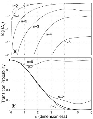
Figure 1: For $A=\frac{\pi}{2}$ and different number of KAM iterations $n$, (a) natural logarithm of the error $\Delta_{n}$ defined in Eq. (59), and (b) transition probabilities $|\langle+1|\psi\rangle|^{2}$ computed numerically (thick line) and $|\langle+1|\psi^{(n)}\rangle|^{2}$ calculated with the KAM algorithm (thin lines) as a function of $\epsilon$, at the end of the pulse.

Figure 1a displays the accuracy of the KAM algorithm for different number of iterations as a function of $\epsilon$ in the case where the pulse area $A=\frac{\pi}{2}$, which corresponds to a peak amplitude equal to $\pi$. One can see that this procedure reproduces the numerical results with great accuracy for any value of $\epsilon$ provided a sufficient (yet small) number of iterations is used. For the range of $\epsilon$ shown on Fig. 1, the fifth iteration is indistinguishable from the numerical result. For $\epsilon=0$, the peak amplitude considered here leads to a complete population transfer from the lower to the upper state (the so-called “$\pi-$ pulse” transfer). Figure 1b shows that this transfer decreases for larger $\epsilon$ until becoming negligible beyond $\epsilon\approx 5$, a feature which characterizes the adiabatic regime. It is striking that the adiabatic regime can be reached with great accuracy from the third iteration on.

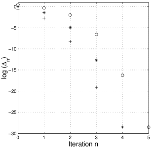
Figure 2: Natural logarithm of the error $\Delta_{n}$ as a function of the number $n$ of KAM iterations for $A=\frac{\pi}{2}$ and $\epsilon=0.5$ (crosses), 1 (stars) and 2 (circles).

The accuracy of the KAM algorithm is plotted as a function of the number of iterations in Figure 2. As suggested by the order $\epsilon^{2^{n}}$ of the remainder, the error decreases faster than exponentially.

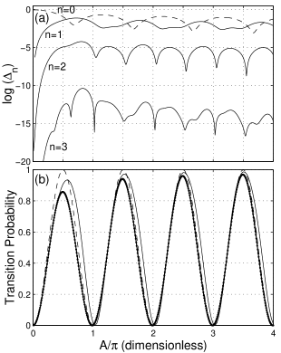
Figure 3: For $\epsilon=1$ and different KAM iterations $n$, (a) natural logarithm of $\Delta_{n}$, and (b) transition probabilities computed numerically (thick line) and with the KAM algorithm ($n=0$: dashed line, $n=1$: thin full line, $n=2$: dotted line, superimposed on the numerical solution) as a function of $A/\pi$, at the end of the pulse.

Figure 3 displays the accuracy of the KAM algorithm as a function of the pulse area $A$. As expected by inspection of the Schrödinger equation (51), Fig. 3b shows that for larger pulse area the pulse is effectively more sudden, since the transition probability can reach maximum values closer to 1. The KAM algorithm accuracy is consequently globally better, except for pulse area smaller than $\pi/2$, as seen on Fig. 3a.

IV Conclusion

We have derived a unitary superconvergent algorithm, based on the KAM technique, that allows to treat time-dependent perturbations that are localized in time. In the physically relevant case of perturbations that are switched on at some finite time in the past, we have shown that the computation of the KAM transformations can be greatly simplified. The remarkable efficiency of the method has been shown for a pulse-driven two-level system, for which we obtain convergence all the way from the sudden regime to the opposite adiabatic regime. We anticipate interesting applications of this method in the context of alignment and orientation of molecules by pulsed laser fields.

Appendix A KAM algorithm in the extended Hilbert space

A.1 $\overline{\mathcal{V}}^{\mathcal{K}}(s)$ and $\widehat{\mathcal{V}}^{\mathcal{K}}(s)$

For time-dependent problems, the KAM algorithm involves calculating the following transforms of operators $\mathcal{V}(s)$ with respect to the propagator of $\mathcal{K}=\mathcal{H}(s)-i\frac{\partial}{\partial s}\otimes\openone_{\mathbb{H}}$ on the extended Hilbert space $\mathbb{K}=\mathbb{L}\otimes\mathbb{H}$:

$$\overline{\mathcal{V}}^{\mathcal{K}}(s)\!\! \equiv \!\!\lim_{T\rightarrow\infty}\frac{1}{T}\int_{0}^{T}\!\!\!\mathrm{d}t\,e^{-it\mathcal{K}}\mathcal{V}(s)e^{it\mathcal{K}}\,,$$ (60a)

$$\widehat{\mathcal{V}}^{\mathcal{K}}(s)\!\! \equiv \!\!\lim_{T\rightarrow\infty}\frac{1}{T}\int_{0}^{T}\!\!\!\mathrm{d}t^{\prime}\!\int_{0}^{t^{\prime}}\!\!\!\mathrm{d}t\,e^{-it\mathcal{K}}\left(\mathcal{V}(s)-\overline{\mathcal{V}}^{\mathcal{K}}(s)\right)e^{it\mathcal{K}}.$$

(60b)

Hence, one has to consider operators on $\mathbb{K}$ of the form $\mathcal{B}(s,t)\equiv e^{-it\mathcal{K}}\mathcal{A}(s)e^{it\mathcal{K}}$ with $\mathcal{A}\equiv\mathcal{V}$ for $\overline{\mathcal{V}}^{\mathcal{K}}$ and $\mathcal{A}\equiv\mathcal{V}-\overline{\mathcal{V}}^{\mathcal{K}}$ for $\widehat{\mathcal{V}}^{\mathcal{K}}$. Using Eq (16), $\mathcal{B}(s,t)$ becomes

$$\mathcal{B}(s,t)\! = \!{\sf T}_{-t}\mathcal{U}_{\mathcal{H}}(t,0;s)\mathcal{A}(s)\mathcal{U}_{\mathcal{H}}^{\dagger}(t,0;s){\sf T}_{t}$$ (61)

$$= \!\mathcal{U}_{\mathcal{H}}(t,0;s-t)\mathcal{A}(s-t)\mathcal{U}_{\mathcal{H}}^{\dagger}(t,0;s-t)$$

$$= \!\mathcal{U}_{\mathcal{H}}(0,-t;s)\mathcal{A}(s-t)\mathcal{U}_{\mathcal{H}}^{\dagger}(0,-t;s)\,,\ \$$

where we used the definition of the translation operator and Eq. (15) to obtain the second and third equalities, respectively.

At the $n$-th iteration of the KAM algorithm, Eqs. (19) imply taking $\mathcal{K}\equiv\mathcal{K}^{{\rm e}}_{n-1}$ and $\mathcal{V}\equiv\mathcal{V}_{n}$ in Eqs. (A.1), hence $\mathcal{U}_{\mathcal{\mathcal{H}}}\equiv\mathcal{U}_{\mathcal{\mathcal{H}}^{{\rm e}}_{n-1}}$ in Eq. (61).

A.2 $\mathcal{U}_{\mathcal{H}^{{\rm e}}_{n}}(t,t_{0};s)$

We show here that the operator $\mathcal{U}_{\mathcal{H}^{{\rm e}}_{n}}(t,t_{0};s)$ can be calculated according to Eq. (22a), or equivalently Eq. (22b), in terms of $U_{H_{0}}(t,t_{0})$ and the operators $\mathcal{S}_{k}(t,t_{0};s)$ with $1\leq k\leq n$ defined by Eq. (23). Indeed, applying Eq. (16) to the propagator of $\mathcal{K}^{{\rm e}}_{n}$ defined by Eqs. (19) yields

$$\mathcal{U}_{\mathcal{H}^{{\rm e}}_{n}}(t,t_{0};s)\! = \!{\sf T}_{t}\mathcal{U}_{\mathcal{K}^{{\rm e}}_{n}}(t,t_{0}){\sf T}_{-t_{0}}$$ (62)

$$= \!{\sf T}_{t}\mathcal{U}_{\mathcal{K}^{{\rm e}}_{n-1}}(t,t_{0})\mathcal{S}_{n}(t,t_{0};s){\sf T}_{-t_{0}}$$

$$= \!{\sf T}_{t}\mathcal{U}_{\mathcal{K}^{{\rm e}}_{n-1}}(t,t_{0}){\sf T}_{-t_{0}}\mathcal{S}_{n}(t,t_{0};s+t_{0})$$

$$= \!\mathcal{U}_{\mathcal{H}^{{\rm e}}_{n-1}}(t,t_{0};s)\mathcal{S}_{n}(t,t_{0};s+t_{0}),\qquad$$

which proves Eq. (22a). Note that by construction $[\mathcal{K}^{{\rm e}}_{n-1},\overline{\mathcal{V}_{n}}^{\mathcal{K}^{{\rm e}}_{n-1}}(s)]=0$, which is crucial for writing the second equality. This commutation relation also allows to permute $\mathcal{U}_{\mathcal{K}^{{\rm e}}_{n-1}}$ and $\mathcal{S}_{n}$ on the second line of Eqs. (62), which then results in Eq. (22b).

Appendix B Averaging for pulse-driven systems

In this appendix, we consider the case of a time-dependent operator $V(t)$ which, before some finite time $t_{{\rm i}}$, is constant in time and commutes with the propagator of an Hamiltonian $H(t)$ on $\mathbb{H}$:

$$V(t)=V(t_{{\rm i}})\quad\forall t\leq t_{{\rm i}},$$ (63a)

$$\left[V(t_{{\rm i}}),U_{H}(t,t_{0})\right]=0\quad\forall t,t_{0}\leq t_{{\rm i}}.$$ (63b)

After $t_{{\rm i}}$ the dependence on time of $V(t)$ is arbitrary provided it is uniformly bounded. We show that the operators $\overline{V}^{H}(t)$ and $\widehat{V}^{H}(t)$, defined by Eqs. (28), can be calculated as

$$\overline{V}^{H}(t)\!\!\! = \!\!\!U_{H}(t,t_{{\rm i}})V(t_{{\rm i}})U_{H}^{\dagger}(t,t_{{\rm i}}),\qquad$$ (64a)

$$\widehat{V}^{H}(t)\!\!\! = \!\!\!\int_{t_{{\rm i}}}^{t}\!\mathrm{d}u\,U_{H}(t,u)\left[V(u)-\overline{V}^{H}(u)\right]U_{H}^{\dagger}(t,u).\qquad$$ (64b)

We first prove Eq. (64a), rewriting Eq. (28a) as

$$\overline{V}^{H}(t)\! = \!\lim_{T\rightarrow\infty}\frac{1}{T}\int_{t-T}^{t}\!\!\mathrm{d}u\,A(t,u),\$$ (65)

where $A(t,u)\equiv U_{H}(t,u)V(u)U_{H}^{\dagger}(t,u)$. The propagator $U_{H}(t,u)$ can be decomposed into $U_{H}(t,t_{{\rm i}})U_{H}(t_{{\rm i}},u)$. If $u\leq t_{{\rm i}}$ then $U_{H}(t_{{\rm i}},u)$ and $V(u)$ satisfy Eqs. (63) implying

$$A(t,u)=U_{H}(t,t_{{\rm i}})V(t_{{\rm i}})U_{H}^{\dagger}(t,t_{{\rm i}})\quad\forall u\leq t_{{\rm i}}.\qquad$$ (66)

For $t\leq t_{{\rm i}}$ the integration domain in Eq. (65) is such that $A(t,u)$ is given by Eq. (66), resulting thus in Eq. (64a). Notice that this latter reduces to

$$\overline{V}^{H}(t)=V(t_{{\rm i}})\quad\forall t\leq t_{{\rm i}}.$$ (67)

On the other hand, when $t>t_{{\rm i}}$ there is a remaining integral over $u\in[t_{{\rm i}},t]$ which is bounded and independent of $T$, vanishing thus in the limit. The result given in Eq. (64a) follows.

We now turn to the proof of Eq. (64b) and write Eq. (28b) as

$$\widehat{V}^{H}(t)=\lim_{T\rightarrow\infty}\frac{1}{T}\int_{0}^{T}\!\!\!\mathrm{d}t^{\prime}\!\int_{t-t^{\prime}}^{t}\!\!\!\mathrm{d}uB(t,u),\$$ (68)

where

$$B(t,u)\equiv U_{H}(t,u)\left[V(u)-\overline{V}^{H}(u)\right]U_{H}^{\dagger}(t,u).$$ (69)

The case $t\leq t_{{\rm i}}$ is directly proven since $B(t,u)$, which is also the integrand in Eq. (64b), vanishes identically by Eq. (67):

$$\widehat{V}^{H}(t)=0\quad\forall t\leq t_{{\rm i}}.$$ (70)

For $t>t_{{\rm i}}$ splitting the domains of integration in Eq. (68) yields

$$\!\!\!\widehat{V}^{H}(t)=\lim_{T\rightarrow\infty}\frac{1}{T}\left\{\int_{0}^{t-t_{{\rm i}}}\!\!\mathrm{d}t^{\prime}\!\int_{t-t^{\prime}}^{t_{{\rm i}}}\!\!\mathrm{d}uB(t,u)\right.$$

$$\!\!\!\left.+\int_{t-t_{{\rm i}}}^{T}\!\!\mathrm{d}t^{\prime}\!\int_{t-t^{\prime}}^{t_{{\rm i}}}\!\!\mathrm{d}uB(t,u)+\int_{0}^{T}\!\!\mathrm{d}t^{\prime}\!\int_{t_{{\rm i}}}^{t}\!\!\mathrm{d}uB(t,u)\right\}\!.\ \quad$$ (71)

The first double integral being bounded and independent of $T$ does not contribute in the limit whereas the second one vanishes because $B(t,u)=0$ if $u\leq t_{{\rm i}}$. The result of Eq. (64b) comes from the last double integral of Eq. (71).

Finally, we show that if Eqs. (63) are satisfied with $V\equiv V_{1}$ and $H\equiv H_{0}$, then Eqs. (64) hold with $V\equiv V_{n}$ and $H\equiv H^{{\rm e}}_{n-1}$ for any $n\geq 1$. The case $n=1$ follows directly. We prove the case $n>1$ by induction, assuming Eqs. (63) are verified for $n-1$. The operator $V_{n}(t)$ is obtained by Eq. (28c) as a sum of terms involving $\widehat{V_{n-1}}^{H^{{\rm e}}_{n-2}}(t)$, which by Eq. (70) is zero for $t\leq t_{{\rm i}}$. Hence $V_{n}(t)=0$ for $t\leq t_{{\rm i}}$ so that Eqs. (63) hold for $n>1$, which concludes the proof. Notice that for $n>1$ Eq. (64a) yields $\overline{V_{n}}^{H^{{\rm e}}_{n-1}}(s)=0$.

References

• [1] A. Galindo and P. Pascual, Quantum mechanics II (Springer-Verlag, New York, 1991).
• [2] M. V. Berry, Proc. R. Soc. London A 429, 61 (1990).
• [3] K. Drese and M. Holthaus, Eur. Phys. J. D 3, 73 (1998).
• [4] J. C. A. Barata, Ann. Henri Poincaré 2, 963 (2001).
• [5] G. Gallavotti, The Elements of Mechanics (Springer-Verlag, New York, 1983).
• [6] J. Bellissard, Stability and Instability in Quantum Mechanics, in Trends and developments in the eighties, edited by S. Albeverio and Ph. Blanchard (World Scientific, Singapore 1985).
• [7] M. Combescure, Ann. Inst. Poincaré 47, 63 (1987).
• [8] M. Combescure, Ann. Phys. 185, 86 (1988).
• [9] P. Duclos and P. Šťovícek, Commun. Math. Phys. 177, 327 (1996).
• [10] P. Blekher, H. R. Jauslin and J. L. Lebowitz, J. Stat. Phys. 68, 271 (1992).
• [11] H. Sambe, Phys. Rev. A 7, 2203 (1973).
• [12] J. S. Howland, Math. Ann. 207, 315 (1974).
• [13] W. Scherer, Phys. Rev. Lett. 74, 1495 (1995).
• [14] W. Scherer, J. Phys. A 30, 2825 (1997).
• [15] W. Scherer, Phys. Lett. A 233,1 (1997).
• [16] W. Scherer, J. Math. Phys. 39, 2597 (1998).
• [17] H. R. Jauslin, S. Guérin and S. Thomas, Physica A 279, 432 (2000).