Holonomic quantum gates: A semiconductor-based implementation

Abstract

We propose an implementation of holonomic (geometrical) quantum gates by means of semiconductor nanostructures. Our quantum hardware consists of semiconductor macroatoms driven by sequences of ultrafast laser pulses (all optical control). Our logical bits are Coulomb-correlated electron-hole pairs (excitons) in a four-level scheme selectively addressed by laser pulses with different polarization. A universal set of single and two-qubit gates is generated by adiabatic change of the Rabi frequencies of the lasers and by exploiting the dipole coupling between excitons

I Introduction

In the recent years the interest about quantum computation (QC) and quantum information processing (QIP) has been restless growing. Applications of QIP e.g., quantum cryptography and quantum teleportation, have been proposed and verified experimentally. In QC it has been shown that quantum algorithms may speed up some classically intractable problems in computer science shor .

Unfortunately this power inherent to quantum features (i.e., entanglement, state superposition) is difficult to be exploited because quantum states are typically highly unstable : the undesired coupling with the many degrees of freedom of the environment may lead to decoherence and to loss of the information encoded. Another source of error can be the imperfect control of parameters driving the evolution of the system. This can lead to wrong output states. To implement effective QIP techniques these two problems must be faced and solved.

For the problem of decoherence, some methods have been proposed theoretically: via error correcting codes ECC it is possible to find errors induced by the environment and correct them. Other approaches propose to encode information in states that are stable against environmental noise 3 or to eliminate dynamically the noise effects (4 ,5 ). A few quantum hardwares have been proposed for implementation of quantum gates; e.g.: nuclear magnetic resonance chuang , ion traps (cirac , sorensen , molmer , cirac2 ) semiconductor quantum dots (or macroatoms) divincenzo , biolatti ; in each of these implementations we have different gates and different ways of processing information.

A conceptually novel approach is topological computation 6 ,7 in which the gate parameters depends only on global features of the control process, being therefore insensitive to local fluctuations. Though interesting the topological gates proposed so far are quite difficult to realize in practice because they are based on of non-local quantum states of many body systems with complicate interactions.

Another approach that keeps some of the global (geometrical) features of the quantum gates and seems closer to today experimental technology, is the the so-called Holonomic Quantum Computation (HQC) (8 , 9 ). In this paper we shall analyze in a detalied manner a recent proposal for HQC with semiconductor quantum dots paper1 .

We shall start by recalling the basic facts about HQC (Sect. II) and on excitonic transitions in semiconductor macroatoms (Sect. III) In Sect IV we will show how to encode quantum information in excitonic state an how to realize single-qubit gates by means of laser pulses. Two-qubit gates resorting to bi-excitonic shift are illustated in Sect V. Sect. VI contains the conclusions and an appendix is added to improve the self-consistency of the paper.

II Quantum Holonomies

When a quantum state undergoes an adiabatic cyclic evolution, a nontrivial phase factor appears. This is called geometrical phase because it only depends on global properties, i.e, not on the path in the parameter space but only on the swept solid angle. If the evolving state is non-degenerate we have only an Abelian phase (Berry phase berry ), but if it is degenerate we have a non-Abelian operator. Then we can use it to process the quantum information encoded in the state.

More precisely, if we have a family $\mathcal{F}$ of isodegenerate Hamiltonians $H(\lambda)$ depending on $m$ dynamically controllable parameters $\lambda$, we encode the information in a $n-$fold degenerate eigenspace $\mathcal{E}$ of an Hamiltonian $H(\lambda_{0})$. Changing the $\lambda$’s and driving $H(\lambda)$ along a loop we produce a non-trivial transformation of the initial state $|\psi_{0}\rangle\rightarrow U|\psi_{0}\rangle$.

These transformations, called holonomies, are the generalization of Berry’s phase and can be computed in terms of the Wilczek-Zee gauge connection W-Z : $U(C)={\bf P}exp(\oint_{C}A)$ where $C$ is the loop in the parameter space and $A=\sum_{\mu=1}^{m}=A_{\mu}d\lambda_{\mu}$ is the $u(n)-$valued connection. If $|D_{i}(\lambda)\rangle$ ($i=1,...,n$) are the instantaneous eigenstates of $H(\lambda)$, the connection is $(A_{\mu})_{\alpha\beta}=\langle D_{\alpha}|{\partial}/{\partial\Omega^{\mu}}|D_{\beta}\rangle$ ($\alpha$, $\beta=1,...,n$).

It is useful to introduce the curvature $2-$form $F=\sum_{\mu\nu}F_{\mu\nu}dx^{\mu}\wedge dx^{\nu}$ where $F_{\mu\nu}=\partial_{\mu}A_{\nu}-\partial_{\nu}A_{\mu}+[A_{\mu},A_{\nu}]$; $F$ allow us to evaluate the dimension of the holonomy group and when this coincides with the dimension of $U(n)$ we are able to perform universal quantum computation with holonomies.

For computation purposes we note that if the connection components commute $[A_{\mu},A_{\nu}]=0$, the curvature reduces to $F_{\mu\nu}=\partial_{\mu}A_{\nu}-\partial_{\nu}A_{\mu}$ and we can use Stoke’s theorem to compute the holonomies. The holonomic transformation can be calculated easier $U=exp(i\int_{S}F_{\mu\nu}d\lambda_{\mu}\wedge d\lambda_{\nu})$ and depends on the ’flux’ of $F_{\mu\nu}$ through the surface $S$ delimited by $C$. It is now clear that holonomies are associated to geometrical features of the parameter space.

Even if with an holonomy we can build every kind of transformation (logical gate) it is useful to think in terms of few simple gates that constitute an universal set (i.e., which can be composed to obtain any unitary operator).

Many efforts have been made to implement geometrical quantum gates (i.e. nuclear magnetic resonance jones or super-conducting nanocircuits falci ) because they are believed to be fault tolerant for errors due to an imperfect control of parameters preskill , ellinas . Non-adiabatic realizations of Berry’s phase logic gates have been studied as well 15 , 16 ,non_ad . More recently, schemes for the experimental implementation of non-Abelian holonomic gates have been proposed for atomic physics, 17 ion traps DCZ , Josephson junctions 19 , Bose-Einstein condensates 20 and neutral atoms in cavity 21 .

The basic idea is to have a four level $\Lambda$ system with an excited state ($|e\rangle$) connected to a triple degenerate space with the logical qubits ($|0\rangle$ and $|1\rangle$) and an ancilla qubit ($|a\rangle$); the three degenerate state are separately addressed and controlled. The effective interaction Hamiltonian describing the system is (in interaction picture)

$$H_{int}=\hbar|e\rangle(\Omega_{0}\langle 0|+\Omega_{1}\langle 1|+\Omega_{a}\langle a|)+h.c.$$ (1)

$H$ possesses a two degenerate states (called dark states) with $E(t)=0$ and two bright states with $E(t)=\pm\Omega$ ($\Omega=\sqrt{|\Omega_{0}|^{2}+|\Omega_{1}|^{2}+|\Omega_{a}|^{2}}$). At $t=0$ we codify the logical information in one of these dark states (i.e., $|0\rangle$ or $|1\rangle$) and then, changing the Rabi frequencies ($\Omega_{i}$, $i=0,1,a$) we perform a loop in the parameter space ($H(0)=H(T)$). If the adiabatic condition is full-filled at a generic time $t$ the state of the system will be a dark state of $H(t)$ and to the hamiltonian loop will correspond a loop for the state vector. Since for the adiabatic condition the excited state is never populated, the instantaneous dark state will be a superposition of the degenerate states. With this loop we produce a rotation in the degenerate space ($|0\rangle$, $|1\rangle$, $|a\rangle$) starting from a logical qubit and passing through the ancilla qubit. At the beginning and at the end of the cycle we have only logical bits, but after a loop a geometrical operator is applied to them. Since we can diagonalize (1) it is easy to calculate the connection and the holonomy associated to the loop.

We can construct two single qubit gates : $U_{1}=e^{i\phi_{1}|1\rangle\langle 1|}$ (selective phase shift) and $U_{2}=e^{i\phi_{2}\sigma_{y}}$ ($\sigma_{y}=i(|1\rangle\langle 0|-|0\rangle\langle 1|)$). These two gates ($U_{1}$ and $U_{2}$) are non-commutable, so we can construct non-Abelian holonomies since $U_{1}U_{2}\neq U_{2}U_{1}$.

To obtain an universal set of gates we must introduce a two bit gate; since these gates exploit the interaction between two qubits they will depend on the physical systems considered. A common choice (DCZ , paper1 ) is to realize a selective phase shift gate $U_{3}=e^{i\phi_{3}|11\rangle\langle 11|}$.

III Excitonic transitions

In what follows we show that if we can act on a quantum dot with coherent optical (laser) pulses, we can produce Coulomb-correlated electron-hole pairs (excitons) and we deal with an interaction Hamiltonian similar to the one described in (1). By changing the laser parameters along the adiabatic loop, we can produce the same single qubit gates as in DCZ .

In the GaAs-based III-V compounds the six electrons in the valence band are divided in a quadruplet ($\Gamma_{8}$ symmetry) which corresponds to $J_{tot}=3/2$, and a doublet ($\Gamma_{7}$ symmetry) which corresponds to $J_{tot}=1/2$. If we consider a GaAs/AlGaAs quantum dot, the confining potential (along the $z$ growth axis) breaks the symmetry and lifts the degeneracy collins . The states of the quadruplet are separated in $J_{z}=\pm 3/2$ (heavy holes) and $J_{z}=\pm 1/2$ (light holes). The $\Gamma_{7}$ electrons have $J_{z}=\pm 1/2$. We can rewrite the eigenstates of $J_{tot}$ and $J_{z}$ using the $|S\rangle$, $|X\rangle$ , $|Y\rangle$, $|Z\rangle$ states (the four $\Gamma$ point Bloch function, table 1).

If we shine the quantum dot with a laser beam we excite an electron from the valence band to the conduction band. In the dipole approximation we have to calculate the amplitude transition $\langle f|{\bf\epsilon}\cdot{\bf r}|i\rangle$ (where $\epsilon$ is the polarization vector of the electromagnetic wave, $|i\rangle$ and $|f\rangle$ are the initial and final state respectively).

Table 1: $\Gamma_{6}$ (conduction band), $\Gamma_{7}$, $\Gamma_{8}$ periodic part of Bloch function.

$|J_{tot},J_{z}\rangle$	$\Psi$	$\Gamma$
$|\frac{1}{2},\frac{1}{2}\rangle$	$i|S\uparrow\rangle$	$\Gamma_{6}$
$|\frac{1}{2},-\frac{1}{2}\rangle$	$i|S\downarrow\rangle$	$\Gamma_{6}$
$|\frac{3}{2},\frac{3}{2}\rangle$	$\frac{1}{\sqrt{2}}|(X+iY)\uparrow\rangle$	$\Gamma_{8}$ (HH)
$|\frac{3}{2},-\frac{3}{2}\rangle$	$\frac{1}{\sqrt{2}}|(X-iY)\downarrow\rangle$	$\Gamma_{8}$ (HH)
$|\frac{3}{2},\frac{1}{2}\rangle$	$-\sqrt{\frac{2}{3}}|Z\uparrow\rangle+\frac{1}{\sqrt{6}}|(X+iY)\downarrow\rangle$	$\Gamma_{8}$ (LH)
$|\frac{3}{2},-\frac{1}{2}\rangle$	$-\sqrt{\frac{2}{3}}|Z\downarrow\rangle-\frac{1}{\sqrt{6}}|(X-iY)\uparrow\rangle$	$\Gamma_{8}$ (LH)
$|\frac{1}{2},\frac{1}{2}\rangle$	$\frac{1}{\sqrt{3}}|Z\uparrow\rangle+\frac{1}{\sqrt{3}}|(X+iY)\downarrow\rangle$	$\Gamma_{7}$
$|\frac{1}{2},-\frac{1}{2}\rangle$	$\frac{1}{\sqrt{3}}|Z\downarrow\rangle+\frac{1}{\sqrt{3}}|(X-iY)\uparrow\rangle$	$\Gamma_{7}$

The only non-vanishing transition amplitudes for our calculations are $\langle S|x|X\rangle,\langle S|y|Y\rangle,\langle S|z|Z\rangle$.

Using this relation and table 1 we can calculate which transitions are allowed and which ones are forbidden.

First we note that, for states like $|(X+iY)\rangle$, we can have a transition only using ’negative’ circular polarization light ${\bf\epsilon}={\bf\epsilon_{x}}-i{\bf\epsilon_{y}}$.

$$\langle S|{\bf\epsilon}\cdot r|(X+iY)\rangle=\langle S|(x-iy)|(X+iY)\rangle=$$

$$=\langle S|x|X\rangle+\langle S|y|Y\rangle=2\langle S|x|X\rangle$$ (2)

($\langle S|x|X\rangle=\langle S|y|Y\rangle$ for the symmetry of our system).

Using “positive” circularly polarized light we have no transition

$$\langle S|{\bf\epsilon}\cdot r|(X+iY)\rangle=\langle S|(x+iy)|(X+iY)\rangle=$$

$$=\langle S|x|X\rangle-\langle S|y|Y\rangle=0$$ (3)

The latter are called polarizations selection rules (PSR).

We have also to consider the spin wave function in the initial and final state. If the initial state has spin up (down) the final state must have spin up (down) (spin selection rules (SSR)). For example:

$$\langle S|(x-iy)|(X+iY)\rangle\langle\uparrow|\uparrow\rangle=2\langle S|x|X\rangle$$

$$\langle S|(x-iy)|(X+iY)\rangle\langle\uparrow|\downarrow\rangle=0$$ (4)

III.1 Heavy-hole transitions

From table 1 we have the heavy hole and the $\Gamma_{6}$ (conduction band) states; using SSR we can say that the only allowed transitions are

$|\frac{3}{2},\frac{3}{2}\rangle$	=$\frac{1}{\sqrt{2}}|(X+iY)\uparrow\rangle$	$\rightarrow$	$|\frac{1}{2},\frac{1}{2}\rangle$	=$i|S\uparrow\rangle$
$|\frac{3}{2},-\frac{3}{2}\rangle$	=$\frac{1}{\sqrt{2}}|(X-iY)\downarrow\rangle$	$\rightarrow$	$|\frac{1}{2},-\frac{1}{2}\rangle$	=$i|S\downarrow\rangle$

The first transition is produced by “negative” circularly polarized light (we write the corresponding operator as $\sigma^{-}$) and the second transition is produced by “positive” circularly polarized light ($\sigma^{+}$) for the PSR.

In terms of excitons (electron-hole pairs) if we perform a transition with $\sigma^{-}$, we promote an electron with spin $3/2$ of the valence band to the conduction band with spin $1/2$ and we get an exciton with angular momentum $-1$ ($E^{-}$). With $\sigma^{+}$ we promote an electron with spin $-3/2$ of the valence band to the conduction band with spin $1/2$ and we have an exciton with angular momentum $1$ ($E^{+}$).

III.2 Light hole transitions

For the light hole we have more allowed transitions; this is due to the presence of the $|Z\rangle$ states in the wave function. As for the HH transitions, using $\sigma^{\pm}$ we have

$|\frac{3}{2},\frac{1}{2}\rangle$	$\underbrace{\longrightarrow}_{\sigma^{-}}$	$|\frac{1}{2},-\frac{1}{2}\rangle$
$|\frac{3}{2},-\frac{1}{2}\rangle$	$\underbrace{\longrightarrow}_{\sigma^{+}}$	$|\frac{1}{2},\frac{1}{2}\rangle$

These transitions are allowed with circular (positive or negative) polarization (${\bf\epsilon}={\bf\epsilon_{x}}\pm i{\bf\epsilon_{y}}$) and propagation along the $z$ (growth) axis. If we have the wave propagating along the $x$ or $y$ axis and the polarization along $z$ the transition is allowed by PSR. Using also the SSR we get the two allowed transitions:

$$\langle\frac{1}{2},\frac{1}{2}|z|\frac{3}{2},\frac{1}{2}\rangle\sim\langle S|z|Z\rangle$$ (5)

$$\langle\frac{1}{2},-\frac{1}{2}|z|\frac{3}{2},-\frac{1}{2}\rangle\sim\langle S|z|Z\rangle$$ (6)

With the operator $\sigma^{0}$ we have the following transitions

$|\frac{3}{2},\frac{1}{2}\rangle$	$\underbrace{\longrightarrow}_{\sigma^{0}}$	$|\frac{1}{2},\frac{1}{2}\rangle$
$|\frac{3}{2},-\frac{1}{2}\rangle$	$\underbrace{\longrightarrow}_{\sigma^{0}}$	$|\frac{1}{2},-\frac{1}{2}\rangle$

Such transitions with polarization along $z$ have been experimentally observed marzin .

Exciting light-hole electrons with three different kinds of light (left and right circular polarization and polarization along $z$ axis) we can induce three different kinds of transitions with the same energy marzin .

In terms of excitons if we make a transition with $\sigma^{\pm}$, we promote an electron with spin $\mp 1/2$ from the valence band to the conduction band with spin $\pm 1/2$ and we get an exciton with angular momentum $\pm 1$ ($E^{\pm}$). Using light propagating along $x$ or $y$ with $z$ polarization we promote an electron with spin $\pm 1/2$ from the valence band to the conduction band with spin $\pm 1/2$ and we have an exciton with angular momentum $0$ ($E^{0}$).

The allowed transitions and the corresponding energy-level scheme for HH and LH are shown in fig. 1.

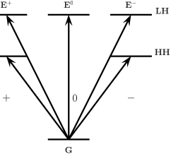
Figure 1: Level scheme for LH and HH.

III.3 $\Gamma_{7}$ transitions

In the same way we can compute the transition selection rules for the $\Gamma_{7}$ electrons.

$|\frac{1}{2},\frac{1}{2}\rangle$	$\underbrace{\longrightarrow}_{\sigma^{-}}$	$|\frac{1}{2},-\frac{1}{2}\rangle$
$|\frac{1}{2},-\frac{1}{2}\rangle$	$\underbrace{\longrightarrow}_{\sigma^{+}}$	$|\frac{1}{2},\frac{1}{2}\rangle$
$|\frac{1}{2},\frac{1}{2}\rangle$	$\underbrace{\longrightarrow}_{\sigma^{0}}$	$|\frac{1}{2},\frac{1}{2}\rangle$
$|\frac{1}{2},-\frac{1}{2}\rangle$	$\underbrace{\longrightarrow}_{\sigma^{0}}$	$|\frac{1}{2},-\frac{1}{2}\rangle$

Like for the LH, we have three different kinds of transitions that can be distinguished by the light polarization.

Those transitions are energetically higher with respect to the LH and HH ones. Therefore, we should be able to inibite them using properly tuned laser sources with bandwidth $\Delta E<E_{\Gamma_{7}}-E_{LH}\simeq 0.3$ eV bastard .

IV Exciton Interaction Hamiltonian and Single Qubit Gates

Now we want to write the interaction Hamiltonian for the exciton transitions (excluding $\Gamma_{7}$ transitions).

The Hamiltonian for the light-matter interaction is (we use the electric field instead of the vector potential schmitt )

$$H_{int}=-e[\vec{P}\cdot\vec{E}^{*}(t)+h.c.]$$ (7)

where $\vec{E}(t)$ is the electric field, $\vec{P}$ is the polarization operator defined as

$$\vec{P}=\sum_{n,m}v_{m}^{\dagger}c_{n}\langle v,m|e\vec{r}|c,n\rangle=\sum_{n,m}v_{m}^{\dagger}c_{n}\vec{\mu}^{*}_{nm}$$ (8)

and

$$\vec{\mu}_{nm}=\langle c,n|e\vec{r}|v,m\rangle$$ (9)

$c_{n}$ and $c_{n}^{\dagger}$ are the annihilation and creation operator for an electron in the conduction band with spin $n$ ($n=\pm 1/2$); $v_{m}$ and $v_{m}^{\dagger}$ are the annihilation and creation operators for an electron in the valence band with spin $m$ ($m=\pm 1/2$ (LH) or $m=\pm 3/2$ (HH) ).

Then, using the dipole approximation ($\vec{E}^{*}(t)=E_{0}e^{i({\bf k}{\bf x}-\omega t)}{\bf\epsilon}\approx E_{0}e^{-i\omega t}{\bf\epsilon}$)

$$H_{int}=-[\sum_{n,m}v_{m}^{\dagger}c_{n}\langle v,m|e\vec{r}|c,n\rangle\cdot\vec{E}^{*}(t)+h.c.]$$ (10)

We define

$$\hbar\Omega_{n,m}=\vec{\mu}_{nm}^{*}\cdot\vec{E}^{*}(t)=E_{0}e^{-i\omega t}{\bf\epsilon}\cdot\langle v,m|e\vec{r}|c,n\rangle$$ (11)

The last term is the dipole transition amplitude.

The term $c_{\pm 1/2}^{\dagger}v_{\pm 3/2}$ describes the promotion of an electron with spin $\pm 3/2$ to the conduction band with spin $\pm 1/2$ and then it describes the creation of an ’heavy’ exciton with angular momentum $\pm 1$ ($E^{\pm}$) from the ground state ($G$). In the same way we can rewrite the terms in (10) taking account of light hole transition. With this new notation, we have non-vanishing coefficients (as discussed in section III) in table 2.

Table 2: Rabi frequencies for allowed transitions.

$\Omega_{n,m}$	v		c	exciton
$\Omega_{\frac{1}{2},\frac{3}{2}}$	$\frac{3}{2}$	$\longrightarrow$	$\frac{1}{2}$	$E^{-}$
$\Omega_{-\frac{1}{2},-\frac{3}{2}}$	$-\frac{3}{2}$	$\longrightarrow$	$-\frac{1}{2}$	$E^{+}$
$\Omega_{\frac{1}{2},-\frac{1}{2}}$	$-\frac{1}{2}$	$\longrightarrow$	$\frac{1}{2}$	$E^{+}$
$\Omega_{-\frac{1}{2},\frac{1}{2}}$	$\frac{1}{2}$	$\longrightarrow$	$-\frac{1}{2}$	$E^{-}$
$\Omega_{\frac{1}{2},\frac{1}{2}}$	$\frac{1}{2}$	$\longrightarrow$	$\frac{1}{2}$	$E^{0}$
$\Omega_{-\frac{1}{2},-\frac{1}{2}}$	$-\frac{1}{2}$	$\longrightarrow$	$-\frac{1}{2}$	$E^{0}$

The Hamiltonian becomes

$$H_{int}=-\hbar[\Omega_{-,\mbox{{\footnotesize HH}}}|E^{-}_{H}\rangle\langle G|+\Omega_{+,\mbox{{\footnotesize HH}}}|E^{+}_{H}\rangle\langle G|+$$

$$\Omega_{+,\mbox{\footnotesize LH}}|E^{+}_{L}\rangle\langle G|+\Omega_{-,\mbox{\footnotesize LH}}|E^{-}_{L}\rangle\langle G|+$$

$$\Omega_{0,\mbox{\footnotesize LH}}|E^{0}_{L}\rangle\langle G|+h.c.]$$ (12)

In the last term we include the two identical kinds of $E^{0}$ excitons.

As we stated before, if we can address the light or heavy hole we can distinguish between $E^{\pm}_{\mbox{{\footnotesize HH}}}$ and $E^{\pm}_{\mbox{{\footnotesize LH}}}$; so using light with specified frequency tuned to LH transition, we can write:

$$H_{int} = -\hbar(\Omega_{+,\mbox{\footnotesize LH}}|E^{+}_{L}\rangle+\Omega_{-,\mbox{\footnotesize LH}}|E^{-}_{L}\rangle+\Omega_{0,\mbox{\footnotesize LH}}|E^{0}_{L}\rangle)\langle G|$$ (13)

$$+ h.c.$$

This Hamiltonian has the same structure as the one proposed in DCZ to implement the holonomic quantum computation with trapped ions. So we can construct the same geometrical single qubit gates ($U_{1}$ and $U_{2}$) using , for example, $E^{+}$ and $E^{-}$ as $|1\rangle$ and $|0\rangle$ bits respectively and $E^{0}$ as ancilla bit $|a\rangle$.

For the first gate we choose $\Omega_{-}=0$, $\Omega_{+}=-\Omega\sin(\theta/2)~{}e^{i\varphi}$ and $\Omega_{0}=\Omega\cos(\theta/2)$. The dark states are given by $|E^{-}\rangle$ and $|\psi\rangle=\cos(\theta/2)|E^{+}\rangle+\sin(\theta/2)~{}e^{i\varphi}|E^{0}\rangle$. By evaluating the connection associated to this two-dimensional degenerate eigenspace, it is not difficult to see that the unitary transformation $U_{1}=e^{i\phi_{1}|E^{+}\rangle\langle E^{+}|}$ ($\phi_{1}=\frac{1}{2}\oint\sin\theta~{}d\theta~{}d\varphi$) can be realized as an holonomy. For the second gate we choose $\Omega_{-}=\Omega\sin\theta\cos\varphi$, $\Omega_{+}=\Omega\sin\theta\sin\varphi$ and $\Omega_{0}=\Omega\cos\theta$. The dark states are now given by $|\psi_{1}\rangle=\cos\theta\cos\varphi|E^{-}\rangle+\cos\theta\sin\varphi|E^{+}\rangle-\sin\theta|E^{0}\rangle$ and $|\psi_{2}\rangle=\cos\varphi|E^{+}\rangle-\sin\varphi|E^{-}\rangle$. In this case, the unitary transformation $U_{2}=e^{i\phi_{2}\sigma_{y}}$ (where $\phi_{2}=\oint\sin\theta d\theta d\varphi$ and $i\sigma=|E^{+}\rangle\langle E^{-}|-|E^{-}\rangle\langle E^{+}|$) can be implemented.

We performed numerical simulations to show how our scheme works and how we can satisfy adiabaticity request and apply logical gates. The exciton states have energies between $1.5~{}eV$ and $1.7~{}eV$ which correspond to sub-femto second time scale; then using femtosecond laser pulse we avoid transition between ground and exciton state during the evolution. Using Rabi frequencies about $0.02$ fs^-1 (corresponding to $\Omega^{-1}=50$ fs) and evolution times of $T_{a}d=7.5$ ps (as in the simulation) we get for the adiabatic condition $\Omega~{}T_{ad}=150\gg 1$ which assures us that there will be no transition between dark and bright states (separated by $\Omega$ energy).

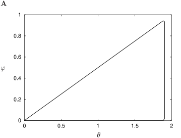
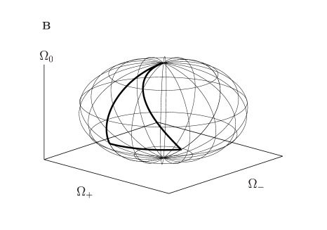
Figure 2: (A) Loop in the $\theta-\phi$ parameter space ($\theta_{m}=\pi$). (B) Evolution of the $|E^{+}\rangle$ in the $|E^{-}\rangle-|E^{+}\rangle-|E^{0}\rangle$ space for gate $2$ and $\phi_{2}=\pi/2$.

In Figure 2(A) the loop in the $\theta-\phi$ space is shown. Since the holonomic operator depends on the solid angle ($\oint d\Omega=\oint d\theta d\phi\sin\theta$), the only contribute from this loop comes from the first part and can be easily calculated $\int d\Omega=1/2(\sin\theta_{m}-\theta_{m}\cos\theta_{m})$. Then it is sufficient to change $\theta_{m}$ to apply a different operator. In Fig. 2 (B) we show the loop in the control parameters manifold for gate 2 ($\Omega^{-}$, $\Omega^{+}$, $\Omega^{0}$), since the parameters are real the 3D vector $\vec{\Omega}$ evolves on a sphere. These two figures refer to the implementation of Hadamard gate (also shown in Fig. 3 (B) and in Fig. (4) ) and we choose $\theta_{m}$ in order to obtain $\oint d\Omega=\pi/4$.

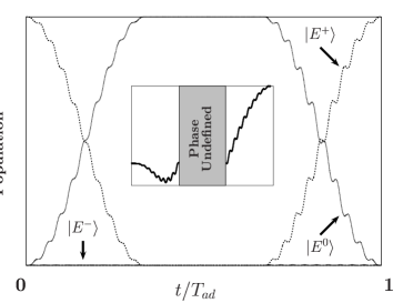
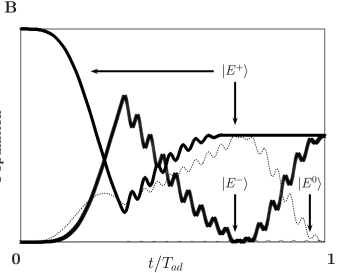
Figure 3: (A) Simulated time evolution of the HQC gate 1 with $\phi_{1}=\pi/4$ and initial state $|E^{+}\rangle$. The inset shows (where it is defined) the quantity $\varphi$ where $\varphi:=\mbox{Arg}\langle\Psi(t)|E^{+}\rangle/|\langle\Psi(t)|E^{+}\rangle|$. (B) Simulated time evolution of the HQC gate 2 with $\phi_{2}=\pi/4$ (Hadamard gate) and initial state $|E^{+}\rangle$.

Figure 3 shows the state populations during the quantum-mechanical evolution; as we can see, the state $|G\rangle$ is never populated (as expected in the adiabatic limit). For the case of gate 1 [see Fig. 3(A)] the $|E^{-}\rangle$ state is decoupled in the evolution while the state $|E^{+}\rangle$ evolves to the ancilla state ($|E^{0}\rangle$), to eventually end in $|E^{+}\rangle$ (as we expect for the dark state). In the inset we show the phase accumulated by the $|E^{+}\rangle$ state; of course, in the central region the phase is undefined.

The quantum evolution of gate 2 in Fig. 3(B) is more complicated because there are not decoupled states and all the three degenerate states are populated. We start from $|E^{+}\rangle$ and end in a superposition of $|E^{+}\rangle-|E^{-}\rangle$. It can be better understood by looking at Fig.  4, where we show the evolution of the dark state in the $|E^{+}\rangle$, $|E^{-}\rangle$, $|E^{0}\rangle$ space. As mentioned above, the initial dark state evolves in the degenerate space: it starts from the $|E^{+}\rangle$ axis, then passes through a superposition of the three states and ends in the $|E^{+}\rangle-|E^{-}\rangle$ plane ($(|E^{+}\rangle+|E^{-}\rangle)/\sqrt{2}$ state).

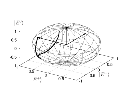
Figure 4: Evolution of the initial state $|E^{+}\rangle$ in the $|E^{-}\rangle-|E^{+}\rangle-|E^{0}\rangle$ space for gate $2$ and $\phi_{2}=\pi/2$.

The numerical simulations show that our scheme works and we are able to produce the desidered gates with realistic parameters for the semiconductor quantum dots 29 and for the recent ultrafast laser technology 26 . Moreover it is clear (also with the gates in paper1 ) that we are able to apply different gates in the same gating time because the latter depends only on the adiabatic constraint (and not on the gate we choose) and though the adiabatic limitation we can apply several quantum gates. Infact recent studies 30 have shown that excitons can exhibit a long dephasing time (comparable to hole-electron recombination time) on nanosecond time-scale. The degeneracy in our model has an importnt role (even if the request can be made weaker and we can use almost-degenerate state i.e. see section IV.1) and this can further prolong the dechoerence time till the recombination of light-hole.

IV.1 Laser bandwidth

We saw that by using light with different polarizations we can induce different transitions and generate $E^{\pm}$, $E^{0}$ excitons. To select which electron to excite (HH, LH, $\Gamma_{7}$) we have to use different energies; in fact the $\Gamma_{7}$ transitions are the most energetic, then there are the LH and the HH.

For circular ($\pm$) polarization light propagating along the $z$ axis we have bastard that the ratio of probabilities to excite the relative electron is

$\frac{\mbox{\footnotesize HH}}{\mbox{\footnotesize LH}}$	=	3
$\frac{\mbox{\footnotesize HH}}{\Gamma_{7}}$	=	$\frac{3}{2}$

So it is sufficient that the laser bandwidth is not too large ($\Delta E<E_{\mbox{\footnotesize LH}}-E_{\mbox{\footnotesize HH}}$ but $\Delta E\ll E_{\Gamma_{7}}-E_{\mbox{\footnotesize LH}}$) to excite HH instead of LH and forbid the $\Gamma_{7}$.

For light propagating along the $x$($y$) axis with $z$ polarization the HH transition are forbidden and

$\frac{\mbox{\footnotesize LH}}{\Gamma_{7}}$	= 2

So even if this laser bandwidth is $\Delta E<E_{\Gamma_{7}}-E_{\mbox{\footnotesize LH}}$ it is more likely to produce LH. As we wrote before in practical situation we should be able to prohibit $\Gamma_{7}$ transition just with this choices.

Now we show that even if we are not able to energetically distinguish HH and LH the holonomic scheme proposed works as usually. The level scheme for this configuration is shown in Fig 5. We can excite $E^{\pm}_{\mbox{\footnotesize HH}}$ excitons or $E^{0}_{\mbox{\footnotesize LH}}$ exciton. If we have an adiabatic evolution fast enough, the three levels are mixed during the evolution and so, for our scheme, they can be considered degenerate.

The energy gap between HH and LH excitons is of the order of $0.05-0.03~{}eV$ ( marzin , miller2 , miller1 , matsumoto ), whereas between $\Gamma_{7}$ and HH-LH the gaps is about $0.3~{}eV$. Both of this energy gap are very large compared to the bandwidth of the pico and femtosecond pulsed laser, so in practical applications one should be able to separate LH and HH excitons.

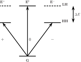
Figure 5: Level scheme for geometrical gates when is impossible to address only HH or LH.

IV.2 Dynamical phase

During the evolution along the adiabatic loop the state acquire a dynamical phase in addition to the geometrical phase. In the first proposal of adiabatic gates with standard two level systems additional work is needed to eliminate this undesidered phase. In ref. ekert they show how this dynamical phase can be eliminated: we have to run the geometrical gate several times in order to let the dynamical phases cancel each others. The drawback in this method is that we have to iterate several times the adiabatic gate and, because of the adiabatic condition, long time is needed to apply the final geometrical gate.

In this model, if we use LH excitons, the logical and the ancilla states are degenerate and the ground state is never populated during the evolution; so the dynamical phase shift is the same for the two logical qubits and can be neglected.

If we encode logical information in the HH excitons ($\pm$) and use the LH exciton ($0$) as ancilla qubit we have an energy difference $\Delta E$ and then a dynamical phase appears. Again, we can neglect it, because at the begining (encoding of information) and at the end (reading information) of the evolution, the $|E^{0}\rangle$ state is never populated and then the phase difference does not affect the logical information. Then, in both models, we can avoid problems with the dynamical phase.

V Two qubits gate

For the two qubit gate we cannot take directly the DCZ model but we use the bi-excitonic shift biolatti . In fact if we have two coupled quantum dots the presence of an exciton in one of them (e.g. in dot b) produces a shift in the energy level of the other (e.g. dot a) from $E$ to $E+\delta/2$.

Let’s consider the two dots in the ground state $|GG\rangle$; if we shine them with circular (’positive’ or ’negative’) light at $E+\delta/2$ energy we should be able to produce two excitons $|EE\rangle$ (see appendix A). For energy conservation this is the only possible transition (the absorption of a single photon is at energy $E$). The detuning allows us to isolate the two-exciton space ($|EE\rangle$) from the single exciton space ($|EG\rangle$, $|GE\rangle$). The level scheme is shown in Fig. 6.

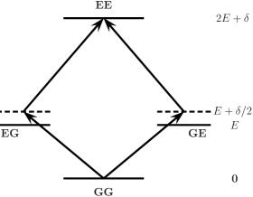
Figure 6: Level scheme for the two-photon process.

To show how the two-photon process happens we solved numerically the Schroedinger equation for a four-level system ($|EE\rangle$, $|EG\rangle$, $|GE\rangle$, $|GG\rangle$). In Fig. 7 (A) we show the population evolution of the states; the Rabi oscillation between $|EE\rangle$ and $|GG\rangle$ are evident and the states $|EG\rangle$, $|GE\rangle$ are never populated. In order to fulfill the perturbation condition we choose $\delta/\Omega=25$.

We have another degree of freedom in our system: the polarization. Shining the dot with circular or linear polarization and we will obtain $|GG\rangle\rightarrow|E^{i}E^{j}\rangle$ ($i,j=+,-,0$) and can reproduce the scheme with polarized excitons. The general Hamiltonian for the two-photon process is (in interaction representation)

$$H_{int}=-\frac{2\hbar^{2}}{\delta}\sum_{i,j=+,-,0}(\tilde{\Omega}_{i}\tilde{\Omega}_{j}e^{i(\phi_{i}+\phi_{j})}|E^{i}E^{j}\rangle\langle GG|+h.c.)$$ (14)

The total two-exciton space has dimension nine but we can restrict to four dimension space turning off two laser with the same polarization (i.e. $-$ or $0$) and because of this situation the scheme is slightly different for the one proposed in the other papers . In ref. paper1 we show how to construct a phase gate; turning on the $+$ and $0$ lasers and modulating them to simulate the evolution in gate $1$ we were able to obtain the geometrical operator $U_{3}=exp(i\phi|E^{+}\rangle\langle E^{+}|^{\otimes 2})$. We can decouple the logical states with negative energy but we still need four laser (two with $+$ polarization and two with $0$ polarization) to produce a loop in the $|E^{+}\rangle^{\otimes 2}-|E^{0}\rangle^{\otimes 2}$ space. The $+$ and $0$ lasers must be resonant with the two-exciton transition, but in this scheme we also produce not-logical states $|E^{+}E^{0}\rangle$ and $|E^{0}E^{+}\rangle$ since have the same energy ($\omega_{i}^{1}+\omega_{j}^{1}=2E+\delta$). Then we have a bigger dark space with dimension three and the scheme is not directly repeated. A detailed calculation of the dark states is given in appendix B.

Now we show how to construct another two-qubit geometrical operator with the same scheme. Since in general an adiabatic loop will produce a superposition of all the dark states, we change laser polarization ($0\rightarrow-$) in order that the system can evolves in the logical space. We note that the space is big enough to produce non-trivial transformation even without the ancilla qubits.

We choose the single laser Rabi frequencies in order to have $\Omega^{++}=\Omega\sin\frac{\theta}{2}$, $\Omega^{--}=\Omega\cos\frac{\theta}{2}$, $\Omega^{+-}=\Omega\sqrt{|\sin\frac{\theta}{2}~{}\cos\frac{\theta}{2}}|$ and $0\leq\theta\leq 4\pi$. The dark state are

$$|D_{1}\rangle = \cos\frac{\theta}{2}|++\rangle-\sin\frac{\theta}{2}|--\rangle$$

$$|D_{2}\rangle = \frac{1}{\sqrt{2}}(|+-\rangle-|-+\rangle)$$

$$|D_{3}\rangle = \sqrt{\frac{|\sin\theta|}{1+|\sin\theta|}}(\sin\frac{\theta}{2}|++\rangle+\cos\frac{\theta}{2}|--\rangle)$$ (15)

$$- \frac{1}{\sqrt{2(1+|\sin\theta|)}}(|+-\rangle+|-+\rangle)$$

The associated connection is

$$A_{\theta}=\left(\begin{array}[]{ccc}0&1/2\sqrt{\frac{|\sin\theta|}{1+|\sin\theta|}}\\ -1/2\sqrt{\frac{|\sin\theta|}{1+|\sin\theta|}}&0\end{array}\right)$$ (16)

Of course, for different values of $\theta~{}$, $[A_{\theta},A_{\theta^{\prime}}]=0$ and we can calculate the loop integral and then the holonomy. From numerical calculation we have $\alpha=\oint 1/2\sqrt{\frac{|\sin\theta|}{1+|\sin\theta|}}d\theta=\int_{0}^{4\pi}1/2\sqrt{\frac{|\sin\theta|}{1+|\sin\theta|}}d\theta=3.6806$ we have for the holonomic operator

$$U=e^{-\alpha\sigma_{x}}=\left(\begin{array}[]{ccc}\cos\alpha&-\sin\alpha\\ \sin\alpha&\cos\alpha\end{array}\right)$$ (17)

We write explicitly the final state using $|D_{1}(4\pi)\rangle=|E^{+}\rangle^{\otimes 2}$ and $|D_{2}(4\pi)\rangle=1/\sqrt{2}(|E^{+}E^{-}\rangle+|E^{-}E^{+}\rangle)$

$$U|E^{+}\rangle^{\otimes 2} = \cos\alpha|E^{+}\rangle^{\otimes 2}$$ (18)

$$- \frac{\sin\alpha}{\sqrt{2}}(|E^{+}E^{-}\rangle+|E^{-}E^{+}\rangle)$$

This is an entangling gate, and then we have another non-trivial gate. In Fig. 7 we show the numerical simulation obtained solving the Schroedinger equation. It is difficult to follow the evolution of the states because of the number of the states populated during the evolution and because of the mixing of them. Moreover it can be noted that the $|GG\rangle$ state never appears in the evolution, the $|E^{-}\rangle^{\otimes 2}$ state is not present at the end of the evolution and the final state is a superposition of $|E^{+}\rangle^{\otimes 2}$ and (symmetrically) $|E^{+}E^{-}\rangle-|E^{-}E^{+}\rangle$.

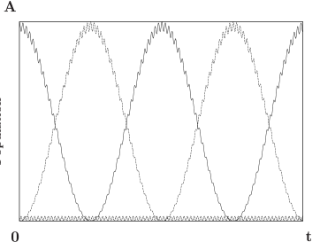
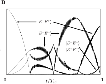
Figure 7: (A) Production of a bi-exciton state and isolation of the $|E^{i}\rangle^{\otimes 2}-|G\rangle^{\otimes 2}$ space with the detuned lasers. (B) Simulated population evolution for the two qubit phase gate.

VI conclusions

In summary, we have shown that geometrical gates can be implemented in quantum dots with optical control. We use polarized excitons to encode logical information and we have been able to construct a universal set of geometrical quantum gates. The biexcitonic shift due to exciton-exciton dipole coupling is exploited to implement two qubit gates. Numerical simulations clearly suggest that one should able to apply several holonomic gates within the decoherence time.

Even though the fault-tolerance features of this geometrical approach has not been completely clarified so far (see e.g., critic ), HQC surely provides, on the one hand, a sort of an intermediate step towards topological quantum computing and on the other hand, it is a natural arena in which explore fascinating quantum phenomena.

Finally we hope that the theoretical investigations here present will be effective in stimulating novel experimental activity in the field of coherent phenomena in semiconductor nanostructures.

Appendix A two-photon process

Here we show how two-photon process may occur in our system. Let’s consider two coupled quantum dots. The energy level spacing in this case is different, in fact the presence of an exciton in one of them (e.g. in dot b) produces a shift in the energy level of the other (e.g. dot a) from $E$ to $E+\delta/2$. We have the following Hamiltonian

$$H_{0}=(2E+\delta)(|E\rangle\langle E|)^{\otimes 2}+$$

$$E(|EG\rangle\langle EG|+|GE\rangle\langle GE|)$$ (19)

Using two lasers with frequencies $\omega=(E+\delta/2)$ ($\hbar=1$) the interaction Hamiltonian is (we explicitly take into account the time dependence $\Omega_{i}=\tilde{\Omega}_{i}e^{-i\omega t}$ from (11))

$$H_{int}=-\hbar\sum_{i=1,2}(\tilde{\Omega}_{i}e^{-i\omega t}|E_{i}\rangle\langle G_{i}|+\tilde{\Omega}_{i}^{*}e^{i\omega t}|G_{i}\rangle\langle E_{i}|)$$ (20)

The effective Hamiltonian for the process is (the apex $2$ indicate that is a second order process)

$$H_{int}^{(2)}=-\hbar\tilde{\Omega}e^{-i\tilde{\omega}t}|E\rangle\langle G|^{\otimes 2}+h.c.$$ (21)

where $\tilde{\omega}=2\omega$ is the frequency that produces the transition between $|GG\rangle$ and $|EE\rangle$. There are four possible states ($|GG\rangle$ ,$|EG\rangle$ ,$|GE\rangle$ , $|EE\rangle$); let the initial state be $|GG\rangle$ and we want to know the amplitude coefficient for the $|GG\rangle\rightarrow|EE\rangle$ (Fig. 6). To do this we use the interaction picture

$$\langle i|e^{iH_{0}t/\hbar}H_{int}e^{-iH_{0}t/\hbar}|j\rangle=$$

$$e^{i(\omega_{i}-\omega_{j})t}e^{\pm i\omega t}\langle i|\tilde{H}_{int}|j\rangle$$ (22)

(the matrix element $\langle i|\tilde{H}_{int}|j\rangle$ is time independent) with the initial conditions $|\psi(0)\rangle=|GG\rangle$ ($|\psi(t)\rangle=\sum c_{ij}(t)|ij\rangle$ , $i,j=E,G$), $\omega^{\prime}=\omega_{EE}-\omega_{m}$ and $\omega^{\prime\prime}=\omega_{m}$, with perturbation theory to the second order we get ($|m\rangle$’s are the intermediate states $|EG\rangle$ and $|GE\rangle$ with energy $E=\hbar\omega_{m}$)

$$c_{EE}^{(2)}(t) = (-\frac{i}{\hbar})^{2}\sum_{m}\int_{0}^{t}d\tau_{1}\langle EE|\tilde{H}_{int}|m\rangle e^{i(\omega^{\prime}-\omega)\tau_{1}}$$ (23)

$$\int_{0}^{\tau_{1}}d\tau_{2}\langle m|\tilde{H}_{int}|GG\rangle e^{i(\omega^{\prime\prime}-\omega)\tau_{2}}$$

Using $\omega^{\prime\prime}+\omega^{\prime}-2\omega=0$ , performing the double integration we get

$$c_{EE}^{(2)}(t)= (-\frac{i}{\hbar})^{2}\sum_{m}\langle EE|\tilde{H}_{int}|m\rangle\langle m|\tilde{H}_{int}|GG\rangle$$ (24)

$$\frac{1}{i(\omega^{\prime\prime}-\omega)}(t-\frac{e^{i(\omega^{\prime}-\omega)t}-1}{i(\omega^{\prime}-\omega)})$$

The term ${1-e^{i(\omega^{\prime}-\omega)t}}{i(\omega^{\prime}-\omega)}$ oscillates, so the leading term is proportional to $t$

$$c_{EE}^{(2)}(t)\approx\frac{i}{\hbar^{2}}\sum_{m}\frac{\langle EE|\tilde{H}_{int}|m\rangle\langle m|\tilde{H}_{int}|GG\rangle}{\omega^{\prime\prime}-\omega}t$$ (25)

Now we go back to the second order Hamiltonian (21) (two-photon process) and calculate the evolution ($\Delta\omega=\omega_{EE}=2\omega$ and $\Delta\omega-\tilde{\omega}=0$ )

$$c_{EE}^{(2)} = -\frac{i}{\hbar}\int_{0}^{t}dt_{1}\langle EE|\tilde{H}_{int}^{(2)}|GG\rangle e^{i(\Delta\omega-\tilde{\omega})t_{1}}=$$ (26)

$$=-\frac{i}{\hbar}\langle EE|\tilde{H}_{int}^{(2)}|GG\rangle\int_{0}^{t}dt_{1}=$$

$$=-\frac{i}{\hbar}(-\hbar\tilde{\Omega})t=i\tilde{\Omega}t$$

The two $c_{EE}^{(2)}$’s are calculated to the same order, so using (24) and (26)

$$\tilde{\Omega}=\frac{1}{\hbar^{2}}\sum_{m}\frac{\langle EE|\tilde{H}_{int}|m\rangle\langle m|\tilde{H}_{int}|GG\rangle}{\omega^{\prime\prime}-\omega}$$ (27)

In our system

$$\langle EE|\tilde{H}_{int}|EG\rangle\langle EG|\tilde{H}_{int}|GG\rangle=$$

$$=\langle EE|\tilde{H}_{int}|GE\rangle\langle GE|\tilde{H}_{int}|GG\rangle=$$

$$=\hbar^{2}\tilde{\Omega}_{1}\tilde{\Omega}_{2}$$ (28)

and we have the Rabi frequency for the two-photon process as function of the single photon process ($\omega^{\prime\prime}_{m}-\omega=\delta/\hbar$).

$$\tilde{\Omega}=\frac{2\hbar\tilde{\Omega}_{1}\tilde{\Omega}_{2}}{\delta}$$ (29)

We take into account the two exciton production for $E^{+}$ and $E^{0}$, and choose : $\tilde{\Omega}_{1i}=\tilde{\Omega}_{i}$, $\tilde{\Omega}_{2i}=\tilde{\Omega}_{i}e^{i\varphi_{i}}$ with $i=+,0$. The phenomenological Hamiltonian (21) became

$$H_{int}=-\frac{2\hbar^{2}}{\delta}\tilde{\Omega}^{2}e^{i\varphi}|E\rangle\langle G|^{\otimes 2}+h.c.$$ (30)

Appendix B Holonomic structure of the two-photon process

To explicitly calculate the dark state of Hamiltonian (14) we change notation and include the phase in the definition of Rabi frequencies $\Omega^{ij}=\tilde{\Omega}_{i}\tilde{\Omega}_{j}e^{i(\phi_{i}+\phi_{j})}$, rewrite the Hamiltonian taking account of production of the same spin excitons ($i=j$) and choose the loop in order to have symmetric Rabi frequencies $\Omega^{ij}=\Omega^{ji}$, we obtain (with $|E^{i}\rangle=|i\rangle$) :

$$H_{int} = -\frac{2\hbar^{2}}{\delta}((\Omega^{++})^{*}|++\rangle+(\Omega^{jj})^{*}|jj\rangle$$ (31)

$$+ (\Omega^{+j})^{*}(|+j\rangle+|j+\rangle)\langle GG|+h.c.$$

where we can take $j=0,-$ to implement to different gates since we reduce the dark space and work with just two polarized excitons.

In addition to the decoupled states which do not appear in 31,

we have three dark states ($\Omega^{2}=|\Omega^{++}|^{2}+|\Omega^{jj}|^{2}$)

$$|D_{1}\rangle = \frac{(\Omega^{jj})^{*}|++\rangle-(\Omega^{++})^{*}|jj\rangle}{\Omega}$$

$$|D_{2}\rangle = \frac{1}{\sqrt{2}}(|+j\rangle-|j+\rangle)$$

$$|D_{3}\rangle = \frac{1}{\Omega\sqrt{|\Omega^{ij}|^{2}+\Omega^{2}/2}}[(\Omega^{ij})^{*}(\Omega^{++}|++\rangle+\Omega^{jj}|jj\rangle)$$ (32)

$$- \frac{\Omega^{2}}{2}(|+j\rangle+|j+\rangle)]$$

Now we can explicitly calculate some connection for particular loops. we choose $j=0$ and for the laser Rabi frequencies $\Omega^{+}_{i}=\sqrt{\Omega\sin(\theta/2)}~{}exp(i\varphi/2)$, $\Omega^{0}_{i}=\sqrt{\Omega\cos(\theta/2)}$ ($i=1,2$ is the dot index) and we use a loop in the $\theta$ and $\phi$ plane similar to the one in figure 2 ($0\leq\theta\leq\pi$ and $0\leq\phi\leq\pi/2$); then we have for the effective Rabi frequencies

$$\Omega^{++} = \Omega\sin\frac{\theta}{2}e^{i\varphi}$$

$$\Omega^{00} = \Omega\cos\frac{\theta}{2}$$

$$\Omega^{+0} = \Omega\sqrt{\sin\frac{\theta}{2}~{}\cos\frac{\theta}{2}}~{}exp(i\varphi/2)$$ (33)

The dark states in 32 explicitly take the form

$$|D_{1}\rangle = \cos\frac{\theta}{2}|++\rangle-\sin\frac{\theta}{2}e^{-i\varphi}||00\rangle$$

$$|D_{2}\rangle = \frac{1}{\sqrt{2}}(|+0\rangle-|0+\rangle)$$

$$|D_{3}\rangle = \sqrt{\frac{\sin\theta}{1+\sin\theta}}(\sin\frac{\theta}{2}e^{i\varphi/2}|++\rangle+\cos\frac{\theta}{2}e^{-i\varphi/2}|00\rangle)$$ (34)

$$- \frac{1}{\sqrt{2(1+\sin\theta)}}(|+0\rangle+|0+\rangle)$$

The connection associated is

$$A_{\theta}=\left(\begin{array}[]{ccc}0&1/2\sqrt{\frac{\sin\theta}{2+\sin\theta}}~{}e^{i\varphi/2}\\ -1/2\sqrt{\frac{\sin\theta}{1+\sin\theta}}~{}e^{-i\varphi/2}&0\end{array}\right)$$ (35)

$$A_{\varphi}=\left(\begin{array}[]{cc}-i\sin^{2}\frac{\theta}{2}&i/2\sqrt{\frac{\sin\theta}{2+\sin\theta}}\sin\theta~{}e^{i\varphi/2}\\ i/2\sqrt{\frac{\sin\theta}{1+\sin\theta}}\sin\theta~{}e^{-i\varphi/2}&i/2\frac{\sin\theta}{1+\sin\theta}\end{array}\right)$$ (36)

The holonomic operator cannot be analytically calculated because the connections do not commute. Then we calculated it with computer simulations by discretization of the loop in the parameter space.