Supersymmetrically transformed
periodic potentials

Abstract. The higher order supersymmetric partners of a stationary periodic potential are studied. The transformation functions associated to the band edges do not change the spectral structure. However, when the transformation is implemented for factorization energies inside of the forbidden bands, the final potential will have again the initial band structure but it can have bound states encrusted into the gaps, giving place to localized periodicity defects.

1 Introduction

Nowadays there is a growing interest in constructing exactly and quasi-exactly solvable potentials which could serve as models in various physical situations (see e.g. [1] and references therein). There exist simple generation techniques, e.g., the supersymmetric quantum mechanics (SUSY QM) and other equivalent procedures as the Darboux transformation, the factorization method, and the intertwining technique [2, 3, 4, 5]. These constructions have been oftenly applied to Hamiltonians having discrete energy levels [6, 7, 8, 9, 10, 11, 12, 13, 14, 15, 16, 17, 18, 19, 20]. However, there are few works involving more general boundary conditions, e.g., on periodic potentials for which the physical solutions of the Schrödinger equation have to be bounded, and hence the spectrum of the Hamiltonian is composed of allowed energy bands separated by the spectral gaps (see e.g. [21]). Our goal in this paper is to show that the SUSY techniques applied to periodic Hamiltonians can produce new solvable potentials [22, 23, 24, 25, 26, 27]. We will see that when the transformation functions are taken as unphysical eigenfunctions of the initial Hamiltonian with factorization energies inside of the forbidden bands, new periodic or asymptotically periodic potentials can be generated [28, 29]. The SUSY periodic partners will be produced when Bloch transformation functions $u(x)$ are used, while the non periodic case will arise for the general $u(x)$ (not necessarily in Bloch form). As a byproduct, we will identify an interesting set of Darboux invariant potentials, i.e., those first order SUSY partners which become just a displaced copy of the initial potential [29].

The organization of the paper is as follows. In the second section a brief overview of the first and second order SUSY QM will be presented. Then, some simple facts about systems involving periodic potential will be discussed. The SUSY QM will be then studied as a tool to generate solvable potentials (periodic or asymptotically periodic) from an initial periodic Hamiltonian. The mechanism will be applied to the Lamé potentials, and the paper will end up with a discussion about the Darboux invariance.

2 Intertwining technique

Let us consider the following relationship

$$\tilde{H}B^{\dagger}=B^{\dagger}H,$$ (1)

$$H=-\frac{d^{2}}{dx^{2}}+V(x),$$ (2)

$$\tilde{H}=-\frac{d^{2}}{dx^{2}}+\tilde{V}(x),$$ (3)

in which the operator $B^{\dagger}$ intertwines the two Schrödinger operators $H,\ \tilde{H}$. Hence, if $\psi_{n}$ is an eigenfunctions of $H$ with eigenvalue $E_{n}$, $H\psi_{n}=E_{n}\psi_{n}$, then $\tilde{\psi}_{n}\propto B^{\dagger}\psi_{n}\neq 0$ is an eigenfunction of $\tilde{H}$ with the same eigenvalue, $\tilde{H}\tilde{\psi}_{n}=E_{n}\tilde{\psi}_{n}$.

In case that $B^{\dagger}$ is a first order differential operator

$$B^{\dagger}=-\frac{d}{dx}+\alpha(x,\epsilon),$$ (4)

the Eqs.(1-3) lead to the standard interrelations between $\alpha(x,\epsilon),\ V(x),\ \tilde{V}(x)$:

$$\alpha^{\prime}(x,\epsilon)+\alpha^{2}(x,\epsilon)=V(x)-\epsilon,$$ (5)

$$\tilde{V}(x)=V(x)-2\alpha^{\prime}(x,\epsilon).$$ (6)

The Darboux formulae are obtained by taking $\alpha=[\ln u(x)]^{\prime}$:

$$-u^{\prime\prime}(x)+V(x)u(x)=\epsilon u(x),$$ (7)

$$\tilde{V}(x)=V(x)-2[\ln u(x)]^{\prime\prime}.$$ (8)

Thus, a new solvable potential $\tilde{V}(x)$ can be efficiently generated from $V(x)$ if one is able to solve explicitly (5) or (7) for a certain $\epsilon$, where $\epsilon$ is called factorization constant because $H$ and $\tilde{H}$ admit the following factorizations:

$$H=BB^{\dagger}+\epsilon,$$ (9)

$$\tilde{H}=B^{\dagger}B+\epsilon.$$ (10)

Notice that $u(x)$ have to be nodeless inside the domain of $x$ in order to avoid the creation of extra singularities of $\tilde{V}(x)$ with respect to $V(x)$. This immediately leads to the typical restriction in the first order case, $\epsilon\leq E_{0}$, where $E_{0}$ is the ground state energy of $H$.

The eigenvalues $E_{n}$ of $H$ for which $B^{\dagger}\psi_{n}\neq 0$ belong to the spectrum of $\tilde{H}$. The rest of Sp($\tilde{H}$) depends on the kernel of $B$, $B\tilde{\psi}_{\epsilon}=0$. The solution of this last equation, $\tilde{\psi}_{\epsilon}\propto 1/u(x)$, is an eigenfunction of $\tilde{H}$ with eigenvalue $\epsilon$. According to the normalizability of the non-singular $\tilde{\psi}_{\epsilon}$, we observe three different cases:

• If $\epsilon=E_{0}$ and $u(x)=\psi_{0}(x)$, it turns out that $\tilde{\psi}_{\epsilon}$ is non-normalizable $\Rightarrow{\rm Sp}(\tilde{H})=\{E_{n},n=1,2,\dots\}$ (the level $E_{0}$ is ‘deleted’ in order to get $\tilde{V}(x)$).

• If $\epsilon<E_{0}$ and non-normalizable $\tilde{\psi}_{\epsilon}$ can be found $\Rightarrow{\rm Sp}(\tilde{H})=\{E_{n},n=0,1,\dots\}$ (the strictly isospectral case).

• If $\epsilon<E_{0}$ and normalizable $\tilde{\psi}_{\epsilon}$ can be found $\Rightarrow{\rm Sp}(\tilde{H})=\{\epsilon,E_{n},n=0,1,\dots\}$ (a level is ‘created’ at $\epsilon$ in order to get $\tilde{V}(x)$).

Suppose now that $B^{\dagger}$ is a second order differential operator:

$$B^{\dagger}=\frac{d^{2}}{dx^{2}}+\beta(x)\frac{d}{dx}+\gamma(x).$$ (11)

By using again (1-3), a pair of equations generalizing (5-6) are found [9, 10]:

$$\frac{\beta^{\prime\prime}}{2\beta}-\left(\frac{\beta^{\prime}}{2\beta}\right)^{2}-\beta^{\prime}+\frac{\beta^{2}}{4}+\left(\frac{\epsilon_{1}-\epsilon_{2}}{2\beta}\right)^{2}+\frac{\epsilon_{1}+\epsilon_{2}}{2}=V(x),$$ (12)

$$\hskip 85.35826pt\tilde{V}(x)=V(x)+2\beta^{\prime}(x).$$ (13)

The solutions of the non-linear second order differential equation (12) can be found either in terms of those of the Riccati equation (5), $\alpha(x,\epsilon_{1}),\ \alpha(x,\epsilon_{2})$, or of those of the Schrödinger equation (7), $u_{1}(x),\ u_{2}(x)$, $\epsilon_{1}\neq\epsilon_{2}$:

$$\beta(x)=\frac{\epsilon_{1}-\epsilon_{2}}{\alpha(x,\epsilon_{1})-\alpha(x,\epsilon_{2})}=-[\ln W(u_{1},u_{2})]^{\prime}.$$ (14)

Contrasting with the first order SUSY, in which $u_{1}$ and $u_{2}$ should be nodeless, in the second order case the Wronskian $W(u_{1},u_{2})$ has to be free of zeros, although $u_{1}$ and $u_{2}$ could have nodes. Once again, Sp($\tilde{H}$) depends on the normalizability of the two eigenfunctions of $\tilde{H}$ with eigenvalues $\epsilon_{1},\ \epsilon_{2}$ which belong to the Kernel of $B$. Their explicit expressions are:

$$\tilde{\psi}_{\epsilon_{1}}\propto\frac{u_{2}(x)}{W(u_{1},u_{2})},\quad\tilde{\psi}_{\epsilon_{2}}\propto\frac{u_{1}(x)}{W(u_{1},u_{2})}.$$ (15)

Different cases can be reported:

• If $\epsilon_{1}=E_{i}$, $u_{1}=\psi_{i}$, $\epsilon_{2}=E_{i+1}$, $u_{2}=\psi_{i+1}$, the two $\tilde{\psi}_{\epsilon_{1}}$, $\tilde{\psi}_{\epsilon_{2}}$ are non-normalizable $\Rightarrow{\rm Sp}(\tilde{H})=\{E_{0},\dots,E_{i-1},$ $E_{i+2},\dots\}$.

• If $\epsilon_{1}<\epsilon_{2}<E_{0}$ and one can find normalizable $\tilde{\psi}_{\epsilon_{1}}$ , $\tilde{\psi}_{\epsilon_{2}}$ $\Rightarrow{\rm Sp}(\tilde{H})=\{\epsilon_{1},\epsilon_{2},E_{n},\\ n=0,1,2,\dots\}$.

• If $E_{i}<\epsilon_{1}<\epsilon_{2}<E_{i+1}$ and one can find normalizable $\tilde{\psi}_{\epsilon_{1}}$ , $\tilde{\psi}_{\epsilon_{2}}$ $\Rightarrow{\rm Sp}(\tilde{H})=\{E_{0},\dots,E_{i},\epsilon_{1},\epsilon_{2},E_{i+1},\dots\}$.

The intertwining technique and the supersymmetric quantum mechanics are closely related, namely, the standard SUSY algebra

$$[Q_{i},H_{\rm ss}]=0,\quad\{Q_{i},Q_{j}\}=\delta_{ij}H_{\rm ss},\quad i,j=1,2,$$ (16)

is simply realized by identifying

$$Q_{1}=\frac{1}{\sqrt{2}}(Q^{\dagger}+Q),\quad Q_{2}=\frac{1}{i\sqrt{2}}(Q^{\dagger}-Q),$$

$$Q=\left(\matrix{0&0\cr B&0}\right),\quad Q^{\dagger}=\left(\matrix{0&B^{\dagger}\cr 0&0}\right),$$

$$H_{\rm ss}=\left(\matrix{B^{\dagger}B&0\cr 0&BB^{\dagger}}\right).$$

The first order SUSY QM arises if $B^{\dagger}$ is the first order operator of (4), and thus $H_{\rm ss}$ is linear in the matrix operator $H^{p}=\left(\matrix{\tilde{H}&0\cr 0&H}\right)$:

$$H_{\rm ss}=(H^{p}-\epsilon).$$ (17)

On the other hand, the second order SUSY (SUSUSY) QM arises if $B^{\dagger}$ is the second order operator (11). In this case $H_{\rm ss}$ becomes quadratic in $H^{p}$ [9, 10]:

$$H_{\rm ss}=(H^{p}-\epsilon_{1})(H^{p}-\epsilon_{2}).$$ (18)

In general, in the higher order SUSY QM $B^{\dagger}$ is an $n$-th order differential operator, $n>1$; in this paper we consider just the cases of first and second order.

3 Schrödinger equation with
periodic potentials

For periodic potentials $V(x+T)=V(x)$ it is convenient to work with the stationary Schrödinger equation in the matrix form:

$$\frac{d}{dx}\left[\begin{array}[]{c}\psi\\ \psi^{\prime}\end{array}\right]=\left[\begin{array}[]{cc}0&1\\ V(x)-E&0\end{array}\right]\left[\begin{array}[]{c}\psi\\ \psi^{\prime}\end{array}\right].$$ (19)

There is a linear mapping ‘propagating’ the solution from a fixed point (let us say $x=0$) to an arbitrary point $x$:

$$\left[\begin{array}[]{c}\psi(x)\\ \psi^{\prime}(x)\end{array}\right]=b(x)\left[\begin{array}[]{c}\psi(0)\\ \psi^{\prime}(0)\end{array}\right].$$ (20)

The $2\times 2$ symplectic matrix $b(x)$ is called transfer matrix. The general behaviour of $\psi$ and the spectrum of $H$ depend on the eigenvalues of the Floquet matrix $b(T)$, which in turn are determined by the discriminant of $b(T)$, $D=D(E)={\rm Tr}[b(T)]$:

$$\beta^{2}-D\beta+1=0\quad\Rightarrow\quad\beta_{\pm}=D/2\pm\sqrt{D^{2}/4-1},\quad\beta_{+}\beta_{-}=1.$$ (21)

The Bloch functions are particular solutions of (19) arising if $[\psi(0),\psi^{\prime}(0)]^{T}$ is one of the eigenvectors of $b(T)$, i.e.,

$$\psi(T)=\beta\psi(0),\quad\psi^{\prime}(T)=\beta\psi^{\prime}(0).$$ (22)

According to the values of $D(E)$, three different physical behaviours are observed:

• $|D(E)|<2$. It turns out that $\beta_{\pm}\in{\mathbb{C}}$, $|\beta_{\pm}|=1$. This implies that any solution (20) is bounded, and hence $E$ belongs to an allowed energy band.

• $|D(E)|=2$. Both $\beta_{+}$ and $\beta_{-}$ become either $+1$ or $-1$, and the associated Bloch functions are periodic or antiperiodic respectively. The Floquet matrix $b(T)$ is degenerated, and the values of $E$ for which $|D(E)|=2$, denoted as

  $$E_{0}<E_{1}\leq E_{1^{\prime}}<\ldots<E_{j}\leq E_{j^{\prime}}<\ldots$$

  define the band edges (which belong also to the spectrum of $H$).

• $|D(E)|>2$. Now $\beta_{\pm}\in{\mathbb{R}}$, implying that the solutions of (20) are unbounded. Hence, $E$ belongs to a forbidden energy band.

4 Supersymmetrically transformed
periodic potentials

It is straightforward to apply the SUSY techniques of section 2 to the periodic potentials of section 3 in order to generate solvable potentials from a given initial one. Let us employ first as transformation functions the periodic or antiperiodic Bloch functions associated to the band edges. The results are the following:

• 1-SUSY using the ‘ground state’ eigenfunction $\psi_{0}$ [23, 24]. It turns out that $\tilde{V}(x)$ is non-singular and periodic. As $B^{\dagger}$ maps bounded eigenfunctions of $H$ into bounded ones of $\tilde{H}$, unbounded into unbounded, etc. $\Rightarrow$ $\tilde{H}$ and $H$ have the same band structure.

• SUSUSY employing the band edge eigenfunctions $\psi_{j},$ $\psi_{j^{\prime}}$ bounding the energy gap $(E_{j},E_{j^{\prime}})$ [25]. The Wronskian becomes nodeless and periodic $\Rightarrow$ $\tilde{V}(x)$ is periodic. Once again $B^{\dagger}$ transforms bounded eigenfunctions of $H$ into bounded ones of $\tilde{H}$, etc. $\Rightarrow$ $H$ and $\tilde{H}$ have the same band structure.

A generalization employing Bloch functions with $\epsilon$ inside of a forbidden energy band can be easily implemented. We distinguish some interesting cases:

• 1-SUSY using Bloch eigenfunctions for $\epsilon\in(-\infty,E_{0})$ [22]. Those eigenfunctions are nodeless, leading to a non-singular periodic superpotential $\alpha(x)$ $\Rightarrow$ $\tilde{H}$ and $H$ have the same band structure.

• SUSUSY employing two nodeless Bloch eigenfunctions associated to $\epsilon_{1},\epsilon_{2}$ which belong to $(-\infty,E_{0})$ [28, 29]. It turns out that $\beta(x)$ is non-singular and periodic $\Rightarrow\ \tilde{H}$ and $H$ have the same band structure.

• SUSUSY using two Bloch eigenfunctions with nodes for $\epsilon_{1},\epsilon_{2}$ such that $E_{j}<\epsilon_{1}<\epsilon_{2}<E_{j^{\prime}}$ [28, 29]. Once again $\beta(x)$ becomes non-singular and periodic $\Rightarrow\ \tilde{H}$ and $H$ have the same band structure.

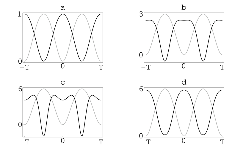
Figure 1: The Lamé potentials (gray curves) of parameter $m=1/2$ and their periodic SUSY partners (black curves) generated by employing physical band edge eigenfunctions: a-c) 1-SUSY for $\epsilon=E_{0}$ and $n=1,2,3$ respectively; d) SUSUSY for $\epsilon_{1}=E_{1},\ \epsilon_{2}=E_{1^{\prime}}$ and $n=3$.

Let us see next what happens when general (non-Bloch) eigenfunctions of $H$ are employed as transformation functions [28, 29].

• 1-SUSY using non-Bloch solutions of (19) for $\epsilon\in(-\infty,E_{0})$. It turns out that nodeless $u$ can be found such that $\tilde{\psi}_{\epsilon_{1}}$ is normalizable. The new potential $\tilde{V}(x)$ has a local nonperiodicity but it is asymptotically periodic. The operator $B^{\dagger}$ maps bounded eigenfunctions of $H$ into bounded ones of $\tilde{H}$, unbounded into unbounded $\Rightarrow\ \tilde{H}$ and $H$ have the same band spectrum but there is a bound state of $\tilde{H}$ at $\epsilon$.

• SUSUSY employing two non-Bloch eigenfunctions for $\epsilon_{1},\epsilon_{2}$ such that $\epsilon_{1}<\epsilon_{2}<E_{0}$. $u_{1},u_{2}$ can be selected such that $\beta$ is non-singular and $\tilde{\psi}_{\epsilon_{1}}$, $\tilde{\psi}_{\epsilon_{2}}$ are normalizable. $\tilde{V}(x)$ presents local nonperiodicities but it is asymptotically periodic. As $B^{\dagger}$ maps bounded eigenfunctions of $H$ into bounded ones of $\tilde{H}$, etc. $\Rightarrow$ $\tilde{H}$ and $H$ have the same band structure but there are two bound states of $\tilde{H}$ at $\epsilon_{1},\epsilon_{2}$.

• A similar SUSUSY procedure with $\epsilon_{1},\ \epsilon_{2}$ such that $E_{j}<\epsilon_{1}<\epsilon_{2}<E_{j^{\prime}}$ can ‘create’ two bound states inside the spectral gap $(E_{j},E_{j^{\prime}})$.

A nice illustration of the SUSY techniques is given by the Lamé potentials:

$$V(x)=n(n+1)m{\rm sn}^{2}(x|m),\quad n\in{\bf N},$$ (23)

where ${\rm sn}(x|m)$ is a standard Jacobi elliptic function of parameter $m\in[0,1]$. The spectrum of $H$ has $2n+1$ band edges defining $n+1$ allowed and $n+1$ forbidden energy bands. Some results applying the SUSY techniques using the band edge eigenfunctions are shown in figure 1. Examples employing Bloch functions with factorization energies inside of the forbidden energy bands arise in figure 2. Finally, some cases implemented by means of non-Bloch transformation functions are illustrated in figure 3.

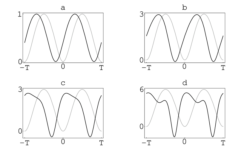
Figure 2: The Lamé potentials (gray curves) with $m=1/2$ and their periodic SUSY partners (black curves) generated by using unphysical Bloch eigenfunctions: a) 1-SUSY with $\epsilon=-1,\ \epsilon<E_{0}$ and $n=1$; b) 1-SUSY with $\epsilon=0.4,\ \epsilon<E_{0}$ and $n=2$; c) SUSUSY with $\epsilon_{1}=1.6,\ \epsilon_{2}=2.9$, $E_{1}<\epsilon_{1}<\epsilon_{2}<E_{1^{\prime}}$ and $n=2$; d) SUSUSY with $\epsilon_{1}=2.3,\ \epsilon_{2}=5$, $E_{1}<\epsilon_{1}<\epsilon_{2}<E_{1^{\prime}}$ and $n=3$.

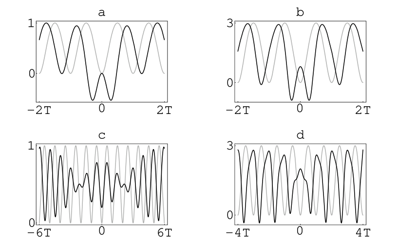
Figure 3: The Lamé potentials (gray curves) with $m=1/2$ and their non-periodic SUSY partners (black curves) generated by using unphysical non-Bloch eigenfunctions: a) 1-SUSY with $\epsilon=0,\ \epsilon<E_{0}$ and $n=1$; b) 1-SUSY with $\epsilon=0.4,\ \epsilon<E_{0}$ and $n=2$; c) SUSUSY with $\epsilon_{1}=1.2,\ \epsilon_{2}=1.3$, $E_{1}<\epsilon_{1}<\epsilon_{2}<E_{1^{\prime}}$ and $n=1$; d) SUSUSY with $\epsilon_{1}=1.51,\ \epsilon_{2}=2.51$, $E_{1}<\epsilon_{1}<\epsilon_{2}<E_{1^{\prime}}$ and $n=2$. All the non-periodic potentials have bound states at the positions of the corresponding $\epsilon$’s.

Let us remark once again that when Bloch transformation functions are used (see figures 1-2), the SUSY partner Hamiltonians $H$ and $\tilde{H}$ have exactly the same spectrum. However, when non-Bloch solutions are employed (see figure 3), the final potential ‘acquires’ bound states encrusted into the forbidden energy bands, which produces local non-periodicities of $\tilde{V}(x)$. These potentials could be useful models for the contact effects in solid state physics.

5 Darboux invariant potentials

Let us notice that for the Lamé potential with $n=1$ the 1-SUSY technique which employs the Bloch functions of either spectral gaps or band edges produces a $\tilde{V}(x)$ which is just the initial potential of a displaced argument, $\tilde{V}(x)=V(x+\delta)$ (see figures 1a and 2a). That phenomenon was discovered by Dunne and Feinberg for the lowest band edge eigenfunction $u(x)=\psi_{0}(x)$ with $\delta=T/2$ (figure 1a), and those potentials were called selfisospectral [23] (see also [25]). Here we observe a more general invariance arising for $n=1$ and $\delta$ arbitrary, which is illustrated in figure 2a. We propose the name translationally invariant under Darboux transformation or simply Darboux invariant potentials [28, 29]. It would be interesting to seek when the 1-SUSY techniques induce that kind of symmetry. The necessary and sufficient condition in order that the Bloch transformation function $u^{\beta}(x)$ will produce a Darboux invariant potential is [25, 28]

$$u^{\beta}(x)u^{1/\beta}(x+\delta)={\rm constant},$$ (24)

where $u^{1/\beta}(x)$ is the second Bloch eigenfunctions associated to the factorization energy $\epsilon$. The restriction (24) is satisfied by the Bloch solutions for the Lamé potentials (23) with $n=1$ but it is not for $n>1$. We should be able to translate the requirement (24) into a restriction onto the form of the potential which is going to be Darboux invariant. By using carefully the 1-SUSY techniques it can be shown that the Weierstrass potentials are the only Darboux invariant potentials [29]. In particular, the Lamé potentials with $n=1$ are included in the Weierstrass family, but there are inside also other interesting non-periodic ones as the 1-soliton well. This result explains why the Lamé potential with $n=1$ is Darboux invariant but those with $n>1$ are not. It has as well shed some light about the general Darboux invariant potentials, not necessarily periodic.

Acknowledgments. The author acknowledges the support of CONACYT, project 32086-E.

References

• [1] J.F. Cariñena, A. Ramos, D.J. Fernández, Ann. Phys. 292, 42 (2001)
• [2] V.B. Matveev, M.A. Salle, Darboux Transformations and Solitons, Springer, Berlin (1991)
• [3] G. Junker, Supersymmetric Methods in Quantum and Statistical Physics, Springer, Berlin (1996)
• [4] B.K. Bagchi, Supersymmetry in Quantum and Classical Mechanics, Chapman & Hall, New York (2001)
• [5] F. Cooper, A. Khare, U. Sukhatme, Supersymmetry in Quantum Mechanics, World Scientific, Singapore (2001)
• [6] B. Mielnik, J. Math. Phys. 25, 3387 (1984)
• [7] D.J. Fernández, Lett. Math. Phys. 8, 337 (1984)
• [8] A.A. Andrianov, N.B. Borisov, M.V. Ioffe, Phys. Lett. A 105, 19 (1984)
• [9] A.A. Andrianov, M.V. Ioffe, V.P. Spiridonov, Phys. Lett. A 174, 273 (1993)
• [10] A.A. Andrianov, M.V. Ioffe, F. Cannata, J.P. Dedonder, Int. J. Mod. Phys. A 10, 2683 (1995)
• [11] D.J. Fernández, J. Negro, M.A. del Olmo, Ann. Phys. 252, 386 (1996)
• [12] D.J. Fernández, Int. J. Mod. Phys. A 12, 171 (1997)
• [13] V.G. Bagrov, B.F. Samsonov, Phys. Part. Nucl. 28, 374 (1997)
• [14] D.J. Fernández, M.L. Glasser, L.M. Nieto, Phys. Lett. A 240, 15 (1998)
• [15] D.J. Fernández, V. Hussin, B. Mielnik, Phys. Lett. A 244, 309 (1998)
• [16] J.O. Rosas-Ortiz, J. Phys. A 31, 10163 (1998); ibid 31, L507 (1998)
• [17] B.F. Samsonov, Phys. Lett. A 263, 274 (2000)
• [18] B. Mielnik, L.M. Nieto, O. Rosas-Ortiz, Phys. Lett. A 269, 70 (2000)
• [19] J.F. Cariñena, A. Ramos, Mod. Phys. Lett. A 15, 1079 (2000)
• [20] J. Negro, L.M. Nieto, O. Rosas-Ortiz, J. Math. Phys. 41, 7964 (2000)
• [21] M. Reed, B. Simon, Methods of Modern Mathematical Physics IV, Academic Press, New York (1978)
• [22] L. Trlifaj, Inv. Prob. 5, 1145 (1989)
• [23] G. Dunne, J. Feinberg, Phys. Rev. D 57, 1271 (1998)
• [24] A. Khare, U. Sukhatme, J. Math. Phys. 40, 5473 (1999)
• [25] D.J. Fernández, J. Negro, L.M. Nieto, Phys. Lett. A 275, 338 (2000)
• [26] B.F. Samsonov, Eur. J. Phys. 22, 305 (2001)
• [27] H. Aoyama, M. Sato, T. Tanaka, M. Yamamoto, Phys. Lett. B 498, 117 (2001)
• [28] D.J. Fernández, B. Mielnik, O. Rosas-Ortiz, B.F. Samsonov, J. Phys. A 35, 4279 (2002)
• [29] D.J. Fernández, B. Mielnik, O. Rosas-Ortiz, B.F. Samsonov, Phys. Lett. A 294, 168 (2002)