Optimization of a Neutron-Spin Test of the Quantum Zeno Effect

Abstract

A neutron-spin experimental test of the quantum Zeno effect (QZE) is discussed from a practical point of view, when the nonideal efficiency of the magnetic mirrors, used for filtering the spin state, is taken into account. In the idealized case the number $N$ of (ideal) mirrors can be indefinitely increased, yielding an increasingly better QZE. By contrast, in a practical situation with imperfect mirrors, there is an optimal number of mirrors, $N_{\text{opt}}$, at which the QZE becomes maximum: more frequent measurements would deteriorate the performance. However, a quantitative analysis shows that a good experimental test of the QZE is still feasible. These conclusions are of general validity: in a realistic experiment, the presence of losses and imperfections leads to an optimal frequency $N_{\text{opt}}$, which is in general finite. One should not increase $N$ beyond $N_{\text{opt}}$. A convenient formula for $N_{\text{opt}}$, valid in a broad framework, is derived as a function of the parameters characterizing the experimental setup.

I Introduction

If very frequent measurements are made on a quantum system in order to ascertain whether it is still in the initial state, its evolution is slowed down and eventually totally hindered in the limit of infinite frequency. This is the quantum Zeno effect (QZE) ref:QZE ; ref:reviewQZE ; ref:QZEMisraSudarshan , that was considered little more than a curiosity until the experimental confirmations by Itano et al. Itano (that followed a theoretical proposal by Cook Cook ) and by Raizen’s group in Texas ref:NonExponentialExp . This last experiment has proved the existence of the QZE for bona fide unstable systems and the occurrence of the inverse QZE, i.e., acceleration of decay by repeated (not extremely frequent) measurements ref:IQZE . The temporal behavior of quantum mechanical systems and in particular the nonexponential features at short times, on which QZE and inverse QZE hinge, are reviewed in Ref. ref:reviewQZE .

We are now going through a phase of experimental verification of the QZE. It is therefore important to understand the physical meaning of “infinitely” frequent measurements, focusing on practical applications, imperfections of the apparatus and experimental losses as well as theoretical bounds. Some of these problems were tackled in Ref. ref:OnQZE . In this article, we reconsider a proposal of an experimental test of the QZE that makes use of neutron spin ref:NeutronSpinTestQZE . In view of the recent progress in perfect crystal neutron-storage technology ref:NeutronStorage1991 ; ref:RauchQZE , it is necessary to investigate the physical properties of a Zeno setup, focusing in particular on practical limits.

In this article we will study the practical imperfections in the spectral decomposition. In a few words, a “spectral decomposition” à la Wigner Wigner is a unitary process that associates additional degrees of freedom to different values of the observable to be measured. In this sense, it yields no wave-function collapse. It is known, and will be reviewed in Sec. II, that a frequent series of spectral decompositions is sufficient in order to obtain a QZE ref:reviewQZE ; ref:NeutronSpinTestQZE ; ref:PetroskyTasakiPrigogine .

In the proposed neutron-spin experimental test of the QZE ref:NeutronSpinTestQZE , the spectral decomposition is realized by a magnetic mirror, with its inevitable imperfections, leading to nonideal efficiency. The main purpose of this article is to quantitatively analyze the consequences of these imperfections: clearly, they tend to deteriorate the performance of the experimental setup; yet, for reasonable values of the experimental parameters ref:NeutronStorage1991 ; ref:RauchQZE , a good test is still clearly feasible with high efficiency. This will be shown in Sec. III, where we will determine an optimum value $N_{\text{opt}}$ of the frequency of measurements: more frequent measurements would simply deteriorate the overall performance of the setup, masking the QZE. These conclusions are of general validity: the presence of losses and imperfections always leads to an optimal frequency, which is in general finite. Our analysis will be extended and generalized in Sec. IV to an arbitrary lossy quantum Zeno experiment, and a convenient formula for $N_{\text{opt}}$ will be derived. We summarize our results in Sec. V.

II Neutron-Spin Test of the QZE with Ideal Mirrors

Let us first briefly review the original proposal of the neutron spin test of the QZE ref:NeutronSpinTestQZE . The basic setup is shown in Fig. 1(a).

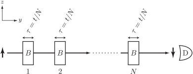
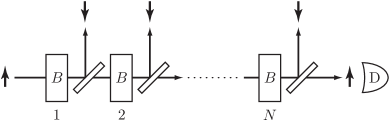
Figure 1: (a) Basic setup for the neutron-spin test of QZE. We set $t/\tau_{\text{Z}}=\pi/2$, so that $2\theta=\pi$. (b) Neutron-spin test of QZE with ideal mirrors.

We prepare, equally spaced along the $y$ axis, $N$ identical regions in each of which a static magnetic field $B$ is applied in the $x$ direction. A neutron wave packet, whose initial spin is oriented in the $z$ direction, travels along the $y$ axis and undergoes a spin rotation at each interaction with the magnetic field, according to the Hamiltonian

$$H=\mu B\sigma_{x},$$ (1)

$\mu$ being the neutron magnetic moment and $\sigma_{i}$ ($i=x,y,z$) the Pauli matrices. The initial state of the incident neutron is $|{S_{0}}\rangle=|{\uparrow}\rangle$ (spin up along the $z$ direction). The final state, after crossing the $N$ regions with the magnetic fields, reads

$$|{S(t)}\rangle=e^{-iHt/\hbar}|{\uparrow}\rangle=\cos\frac{\mu Bt}{\hbar}|{\uparrow}\rangle-i\sin\frac{\mu Bt}{\hbar}|{\downarrow}\rangle,$$ (2)

where $t$ is the total time spent in the magnetic field and we have ignored, for simplicity, the spatial degrees of freedom of the neutron. By defining

$$\theta=\frac{\mu Bt}{\hbar}=\frac{t}{\tau_{\text{Z}}},$$ (3)

where $\tau_{\text{Z}}\,(=\hbar\langle{\uparrow}|H^{2}|{\uparrow}\rangle^{-1/2}$ in this case) is the so-called Zeno time and $2\theta$ the classical precession angle of the spin, the survival probability of the initial state $|{\uparrow}\rangle$ reads

$$P(\theta)=|\langle{\uparrow}|e^{-iHt/\hbar}|{\uparrow}\rangle|^{2}=\cos^{2}\!\theta.$$ (4)

Notice that if $Bt$ is adjusted so as to satisfy

$$\theta=\frac{\pi}{2},$$ (5)

the spin is completely flipped

$$|{S(t)}\rangle=e^{-iHt/\hbar}|{\uparrow}\rangle=-i|{\downarrow}\rangle.$$ (6)

In this case the survival probability of the initial state $|{\uparrow}\rangle$ vanishes

$$P(\theta)=0.$$ (7)

This situation, shown in Fig. 1(a), is that usually considered in the literature. However, the whole analysis that follows identically applies to the general case (3)–(4).

Let us now check, at every step, whether the spin has remained in the initial state $|{\uparrow}\rangle$ despite the spin rotation in the $B$-field. To this end, we insert $N$ magnetic mirrors after every $B$-region, as in Fig. 1(b). The incident neutron undergoes $N$ “spin-measurements” until it reaches the detector D. At each step, if the spin state remains up, the neutron is transmitted through the mirror and keeps traveling right, otherwise it is reflected out by the mirror. Detector D counts those neutrons that have “survived” at each of these $N$ “measurements,” so that the detection probability at D is nothing but the survival probability of the initial state $|{\uparrow}\rangle$.

As clarified in Refs. ref:reviewQZE and ref:NeutronSpinTestQZE , the insertion of a mirror does not represent a measurement of the spin state; it just constitutes a generalized spectral decomposition (GSD) in Wigner’s sense Wigner , namely a (unitary) physical process that associates an “external” degree of freedom (whose role is played here by the wave packet of the neutron) to different values of the observable to be measured (the neutron spin): a frequent sequence of GSD is sufficient for the occurrence of a QZE. In a magnetic field, the spin state of the incident neutron is changed from the initial one $|{\uparrow}\rangle$ to $e^{-iHt/N\hbar}|{\uparrow}\rangle$ and the neutron is then decomposed by the mirror into two branch waves: the spin-up component going rightward and the spin-down one going upward in Fig. 1(b). The state of the neutron just after the first mirror is hence given by

$$|{\psi_{1}}\rangle=\mathcal{T}e^{-iHt/N\hbar}|{\uparrow}\rangle\otimes|{t_{1}}\rangle+\mathcal{R}e^{-iHt/N\hbar}|{\uparrow}\rangle\otimes|{r_{1}}\rangle,$$ (8)

where the spectral decomposition with respect to the spin state is expressed in terms of the projection operators

$$\mathcal{T}=|{\uparrow}\rangle\langle{\uparrow}|,\quad\mathcal{R}=|{\downarrow}\rangle\langle{\downarrow}|$$ (9)

and $|{t_{n}}\rangle$ and $|{r_{n}}\rangle$ are the transmitted and reflected wave packets after the $n$th mirror [and before the $(n+1)$th magnetic field], representing the spatial degrees of freedom of the neutron. Repeating these operations $N$ times, we obtain the final state of the neutron

$$|{\psi_{N}}\rangle = (\mathcal{T}e^{-iHt/N\hbar})^{N}|{\uparrow}\rangle\otimes|{t_{N}}\rangle$$

$${}+\sum_{n=1}^{N}\mathcal{R}e^{-iHt/N\hbar}(\mathcal{T}e^{-iHt/N\hbar})^{n-1}|{\uparrow}\rangle\otimes|{r_{n}}\rangle,$$

so that the probability for the neutron to be detected at detector D, i.e., the survival probability of the initial spin state $|{\uparrow}\rangle$, reads

$$P^{(N)}(\theta)$$

$$\quad=|\{\langle{\uparrow}|\otimes\langle{t_{N}}|\}|{\psi_{N}}\rangle|^{2}=|\langle{\uparrow}|(\mathcal{T}e^{-iHt/N\hbar})^{N}|{\uparrow}\rangle|^{2}$$

$$\quad=|\langle{\uparrow}|e^{-iHt/N\hbar}|{\uparrow}\rangle|^{2N}=\left(\cos\frac{\theta}{N}\right)^{2N},$$ (11)

where we have made use of Eq. (3) (within our approximations, the total duration of the experiment is $t$, with or without magnetic mirrors). Under the condition (5) (and in general for $\theta<\pi/2$), this is nonvanishing for any $N\geq 2$ and is an increasing function of $N$. Frequent “checks” of the spin state slow down the evolution of the initial state $|{\uparrow}\rangle$: the survival probability $P^{(N)}(\theta)$ increases with the frequency of “measurements.” This is a QZE. Furthermore, in the limit of infinite frequency,

$$\lim_{N\to\infty}P^{(N)}(\theta)=1\quad\text{($\theta$ fixed)},$$ (12)

i.e., the spin is frozen and ceases to evolve, in agreement with the theorem by Misra and Sudarshan ref:QZEMisraSudarshan .

An experiment is at present being performed ref:RauchQZE by making use of a recently developed neutron storage technique ref:NeutronStorage1991 . Neutrons with a well-defined energy and in a given spin state are stored in a $1\,\mathrm{m}$ long perfect crystal resonator. The neutrons, at the given energy, satisfy the Bragg reflection condition and bounce back and forth between the two slabs at both ends of the silicon crystal. (At present, neutrons can be reflected a few thousands times with small losses ref:NeutronStorage1991 ; ref:RauchQZE .) In the central part of the resonator, a spin-rotating RF field will be applied, playing the role of the magnetic field in Fig. 1.

The Zeno effect can be obtained as follows. A neutron whose wavelength satisfies the Bragg condition is reflected back by the crystal. However, if a magnetic field is applied at one of the crystal slabs, yielding different potentials for different spin states of the neutron, the neutrons are selected according to their spin state: if, say, a spin-up neutron satisfies the Bragg condition at a plate, the neutron is reflected back and kept inside the resonator; if, on the other hand, the spin is flipped by the spin-rotating RF field, its wavelength does not meet the Bragg condition and the neutron is transmitted out of the resonator. The crystal plates with the magnetic fields play therefore the role of the “magnetic mirrors” in Fig. 1(b), performing the GSDs. Hence, in this experimental setup, the probability for the neutron to remain in the storage apparatus is the survival probability of the initial spin state.

It should be clear by now that it is of primary importance to analyze the effect of losses and imperfections, in order to understand whether the experiment is still meaningful in a realistic situation. Notice that the number $N$ of traverses and interactions should be very large, in order to get a good manifestation of the QZE. This, on the other hand, entails a dramatic (exponential) propagation of “errors.” This will be investigated in the following two sections.

III Neutron-Spin Test of the QZE with Non-Ideal Mirrors

Losses are unavoidable in real experiments and must be duly taken into account. A magnetic mirror, for example, is not ideal, as tacitly assumed in the previous section. It has a nonvanishing probability of failing to correctly decompose the spin state. Assume that the magnetic mirror has transmission $T_{\uparrow(\downarrow)}$ and reflection $R_{\uparrow(\downarrow)}$ coefficients for a spin-up (spin-down) neutron (Fig. 2). (They are in general complex valued and constrained by $|T_{\uparrow(\downarrow)}|^{2}+|R_{\uparrow(\downarrow)}|^{2}=1$.)

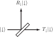
(a)	(b)

Figure 2: Transmission and reflection coefficients for (a) a spin-up neutron and (b) a spin-down neutron.

We assumed in the previous section that $|T_{\uparrow}|=|R_{\downarrow}|=1$ and $R_{\uparrow}=T_{\downarrow}=0$, but this is not the case for actual magnetic mirrors. So the question arises as to whether (and to which extent) it is possible to observe the QZE with non-ideal mirrors. In other words, whether the QZE still takes place if the “measurements” (i.e., the spectral decompositions) are imperfect.

At the $n$th (non-ideal) mirror, the spin-up component of a neutron, $|{\uparrow}\rangle\otimes|{t_{n-1}}\rangle$, is split into two waves

$$|{\uparrow}\rangle\otimes|{t_{n-1}}\rangle\to|{\uparrow}\rangle\otimes\Bigl{(}T_{\uparrow}|{t_{n}}\rangle+R_{\uparrow}|{r_{n}}\rangle\Bigr{)}$$ (13a)

and a similar expression holds for the spin-down component

$$|{\downarrow}\rangle\otimes|{t_{n-1}}\rangle\to|{\downarrow}\rangle\otimes\Bigl{(}T_{\downarrow}|{t_{n}}\rangle+R_{\downarrow}|{r_{n}}\rangle\Bigr{)}.$$ (13b)

(No spin-flip is assumed to occur at the magnetic mirror. The most general case, where such spin-flips take place, is investigated in the Appendix.) The right arrows in Eqs. (13) and in the following stand for the (unitary) physical processes that are responsible for the spectral decomposition. Hence for a neutron in a general spin state $|{S}\rangle$, the magnetic mirror provokes the following spectral decomposition

$$|{S}\rangle\otimes|{t_{n-1}}\rangle \equiv \Bigl{(}c_{\uparrow}|{\uparrow}\rangle+c_{\downarrow}|{\downarrow}\rangle\Bigr{)}\otimes|{t_{n-1}}\rangle$$ (14)

$$\to \Bigl{(}c_{\uparrow}T_{\uparrow}|{\uparrow}\rangle+c_{\downarrow}T_{\downarrow}|{\downarrow}\rangle\Bigr{)}\otimes|{t_{n}}\rangle$$

$${}+\Bigl{(}c_{\uparrow}R_{\uparrow}|{\uparrow}\rangle+c_{\downarrow}R_{\downarrow}|{\downarrow}\rangle\Bigr{)}\otimes|{r_{n}}\rangle$$

$$= \tilde{\mathcal{T}}|{S}\rangle\otimes|{t_{n}}\rangle+\tilde{\mathcal{R}}|{S}\rangle\otimes|{r_{n}}\rangle,$$

where the operators

$$\tilde{\mathcal{T}}=|{\uparrow}\rangle T_{\uparrow}\langle{\uparrow}|+|{\downarrow}\rangle T_{\downarrow}\langle{\downarrow}|,\quad\tilde{\mathcal{R}}=|{\uparrow}\rangle R_{\uparrow}\langle{\uparrow}|+|{\downarrow}\rangle R_{\downarrow}\langle{\downarrow}|$$ (15)

incorporate the effects due to the imperfections of the mirror. These operators $\tilde{\mathcal{T}}$ and $\tilde{\mathcal{R}}$, even though they are no longer projection operators, play the same role as the projection operators $\mathcal{T}$ and $\mathcal{R}$ in the ideal case (8)–(9). The final state of the neutron after the final ($N$th) magnetic mirror is given by

$$|{\tilde{\psi}_{N}}\rangle = (\tilde{\mathcal{T}}e^{-iHt/N\hbar})^{N}|{\uparrow}\rangle\otimes|{t_{N}}\rangle$$

$${}+\sum_{n=1}^{N}\tilde{\mathcal{R}}e^{-iHt/N\hbar}(\tilde{\mathcal{T}}e^{-iHt/N\hbar})^{n-1}|{\uparrow}\rangle\otimes|{r_{n}}\rangle$$

and the probability for the neutron to be detected at detector D reads

$$\tilde{P}^{(N)}(\theta) = \|\langle{t_{N}}|{\tilde{\psi}_{N}}\rangle\|^{2}$$ (17)

$$= \mathop{\mathrm{tr}}\nolimits[(\tilde{\mathcal{T}}e^{-iHt/N\hbar})^{N}\rho_{0}(e^{iHt/N\hbar}\tilde{\mathcal{T}}^{\dagger})^{N}],\quad$$

where $\rho_{0}=|{\uparrow}\rangle\langle{\uparrow}|$ is the initial density operator of the neutron spin. [The spin state observed at the detector is not necessarily $|{\uparrow}\rangle$; it is the probability (17) that one measures in the actual experiment.]

Let us evaluate the probability (17). The eigenvalues $\xi_{\pm}(N)$ of the operator

$$\tilde{\mathcal{T}}e^{-iHt/N\hbar}$$

$$\quad=\frac{1}{2}(T_{\uparrow}+T_{\downarrow})\cos\frac{\theta}{N}-\sigma_{x}\frac{i}{2}(T_{\uparrow}+T_{\downarrow})\sin\frac{\theta}{N}$$

$$\quad\phantom{=}{}+\sigma_{y}\frac{1}{2}(T_{\uparrow}-T_{\downarrow})\sin\frac{\theta}{N}+\sigma_{z}\frac{1}{2}(T_{\uparrow}-T_{\downarrow})\cos\frac{\theta}{N}$$

(18)

are given by

$$\xi_{\pm}(N) = \frac{1}{2}\,\Biggl{[}(T_{\uparrow}+T_{\downarrow})\cos\frac{\theta}{N}$$

$$\phantom{\frac{1}{2}\,\Biggl{[}}{}\pm\sqrt{(T_{\uparrow}+T_{\downarrow})^{2}\cos^{2}\!\frac{\theta}{N}-4T_{\uparrow}T_{\downarrow}}\Biggr{]}.$$

[The eigenvalues $\xi_{\pm}(N)$ will henceforth be written $\xi_{\pm}$, unless confusion arises.] By rewriting the operator (18) as

$$\tilde{\mathcal{T}}e^{-iHt/N\hbar}=\frac{1}{2}(\xi_{+}+\xi_{-})+\frac{1}{2}(\xi_{+}-\xi_{-})\sigma_{n},$$ (20)

where $\sigma_{n}=\bm{n}\cdot\bm{\sigma}$, $\bm{n}$ being a complex-valued vector satisfying $\bm{n}^{2}=n_{x}^{2}+n_{y}^{2}+n_{z}^{2}=1$, we readily obtain

$$(\tilde{\mathcal{T}}e^{-iHt/N\hbar})^{N}=\frac{1}{2}(\xi_{+}^{N}+\xi_{-}^{N})+\frac{1}{2}(\xi_{+}^{N}-\xi_{-}^{N})\sigma_{n}.$$ (21)

A series of elementary calculations yields the following exact expression for the probability

$$\tilde{P}^{(N)}(\theta)$$

$$\quad=\left|A(N)-B(N)T_{\downarrow}\cos\frac{\theta}{N}\right|^{2}+\left|B(N)T_{\downarrow}\sin\frac{\theta}{N}\right|^{2},$$

(22)

with

$$A(N)=\frac{\xi_{+}^{N+1}(N)-\xi_{-}^{N+1}(N)}{\xi_{+}(N)-\xi_{-}(N)},$$ (23a)

$$B(N)=\frac{\xi_{+}^{N}(N)-\xi_{-}^{N}(N)}{\xi_{+}(N)-\xi_{-}(N)}.$$ (23b)

We are now in a position to see whether it is possible to observe the QZE with non-ideal mirrors. In order to analyze its $N$-dependence, let us expand the probability (22) as a function of $|T_{\downarrow}/T_{\uparrow}|\ll 1$. (In the experiment ref:NeutronStorage1991 , $|T_{\downarrow}/T_{\uparrow}|^{2}\lesssim 10^{-4}$.) For any $N\geq 2$, the eigenvalues in Eq. (LABEL:eqn:Eigenvalues) are expanded as

$$\xi_{+}\simeq T_{\uparrow}\cos\frac{\theta}{N}\left[1-\frac{T_{\downarrow}}{T_{\uparrow}}\tan^{2}\!\frac{\theta}{N}+O(T_{\downarrow}^{2}/T_{\uparrow}^{2})\right],$$ (24a)

$$\xi_{-}\simeq\xi_{+}\left[\frac{T_{\downarrow}}{T_{\uparrow}}\left(1+\tan^{2}\!\frac{\theta}{N}\right)+O(T_{\downarrow}^{2}/T_{\uparrow}^{2})\right],$$ (24b)

from which one obtains

$$A(N) = \xi_{+}^{N}\,\biggl{[}1+\frac{\xi_{-}}{\xi_{+}}+\cdots+\left(\frac{\xi_{-}}{\xi_{+}}\right)^{N}\biggr{]}$$

$$\simeq \left(T_{\uparrow}\cos\frac{\theta}{N}\right)^{N}$$

$${}\times\left[1-\frac{T_{\downarrow}}{T_{\uparrow}}\left((N-1)\tan^{2}\!\frac{\theta}{N}-1\right)+\cdots\right]$$

and a similar expansion holds for $B(N)$. We thus easily obtain an approximate expression for the probability (22)

$$\tilde{P}^{(N)}(\theta) \simeq |T_{\uparrow}|^{2N}\left(\cos\frac{\theta}{N}\right)^{2N}$$

$${}\times\left[1-2\mathop{\mathrm{Re}}\!\left(\frac{T_{\downarrow}}{T_{\uparrow}}\right)(N-1)\tan^{2}\!\frac{\theta}{N}+\cdots\right],$$

valid for $N\geq 2$. [For $N=1$, $\tilde{P}^{(N)}(\theta)=\sin^{2}\!\theta\,|T_{\downarrow}|^{2}+\cos^{2}\!\theta\,|T_{\uparrow}|^{2}$ exactly.] It is clear from formula (LABEL:eqn:PExpansion) that the probability $\tilde{P}^{(N)}(\theta)$ is well approximated by

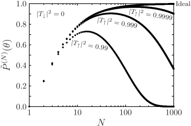
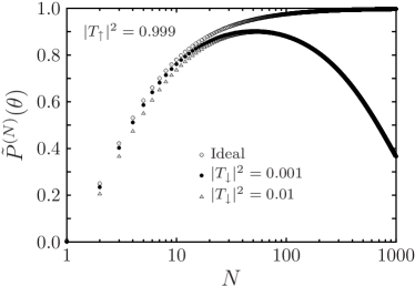
(a)	(b)

Figure 3: (a) $T_{\uparrow}$-dependence and (b) $T_{\downarrow}$-dependence of the probability $\tilde{P}^{(N)}(\theta)$ in Eq. (22). In both figures, $\arg T_{\uparrow}=\arg T_{\downarrow}=0$.

$$\tilde{P}^{(N)}(\theta)\simeq|T_{\uparrow}|^{2N}\left(\cos\frac{\theta}{N}\right)^{2N}.$$ (27)

This shows that neither the transmission coefficient $T_{\downarrow}$ for a spin-down neutron, nor the phases of $T_{\uparrow}$ and $T_{\downarrow}$ bear any important influence on the probability $\tilde{P}^{(N)}(\theta)$; the only relevant quantity is the transmission probability $|T_{\uparrow}|^{2}$. Since $|T_{\uparrow}|^{2}\simeq 1$, for $N$ not too large the factor $|T_{\uparrow}|^{2N}$ is almost unity and the probability $\tilde{P}^{(N)}(\theta)$ behaves like

$$\tilde{P}^{(N)}(\theta)\simeq\left(\cos\frac{\theta}{N}\right)^{2N}\quad\text{($N$ not too large)}.$$ (28)

This is the same as the survival probability with ideal mirrors given in Eq. (11), and is an increasing function of $N$. However, for larger $N$, the factor $[\cos(\theta/N)]^{2N}$ is almost unity, and the probability behaves like

$$\tilde{P}^{(N)}(\theta)\simeq|T_{\uparrow}|^{2N}\quad\text{(larger $N$)},$$ (29)

decreasing exponentially to zero as $N\to\infty$: as the number of mirrors, $N$, is increased, the mirror imperfections ($|T_{\uparrow}|^{2N}<1$) dominate over the increasing factor $[\cos(\theta/N)]^{2N}$, suppressing the QZE for very large $N$. (Clearly, the meaning of “large” $N$ in the two preceding equations must be precisely defined. This will be done in the following.)

There must be therefore an optimal number of mirrors, $N_{\text{opt}}$, in order to observe the QZE if the losses in the “measurement” processes (spectral decompositions) are taken into account. In Fig. 3, the probability $\tilde{P}^{(N)}(\theta)$ computed according to the exact expression (22) is plotted as a function of $N$ for a few values of the transmission coefficients $T_{\uparrow}$ and $T_{\downarrow}$. The figures corroborate the previous discussion. The QZE can be observed even with non-ideal mirrors, if $N$ is not too large, namely if one does not “check” the system’s state too frequently: this is good news from an experimental point of view, since one need not and should not attempt to indefinitely increase the number of mirrors (or reflections in the neutron resonator experiment) in order to achieve an optimal QZE. Notice also that the probability $\tilde{P}^{(N)}(\theta)$ significantly depends on $T_{\uparrow}$, but displays almost no dependence on $T_{\downarrow}$.

It is possible to estimate the optimal number of “measurements,” $N_{\text{opt}}$, yielding the maximum probability $\tilde{P}^{(N_{\text{opt}})}(\theta)$. This can be done from the approximate formula (27) as follows. For actual magnetic mirrors, $|T_{\uparrow}|^{2}$ is almost unity (a reasonable value of $1-|T_{\uparrow}|^{2}$ is of order $10^{-4}$ ref:NeutronStorage1991 ) and $N_{\text{opt}}$ is expected to be large. The maximum of the function $f(x)=a^{x}\cos^{x}(2\theta/x)$, with $a\lesssim 1$, is given by one of the solutions of the equation $a\cos(2\theta/x)=\exp[-(2\theta/x)\tan(2\theta/x)]$ and is approximately $x_{\text{opt}}\simeq 2\theta/\sqrt{\ln a^{-2}}$. Applying this result to the probability (27) one obtains

$$N_{\text{opt}}\simeq\left[\frac{\theta}{\sqrt{1-|T_{\uparrow}|^{2}}}\right]\quad(|T_{\uparrow}|^{2}\simeq 1),$$ (30)

where $[x]$ is the closest integer to $x$. The maximum is then readily evaluated

$$\tilde{P}^{(N_{\text{opt}})}(\theta) \simeq 1-\frac{2\theta^{2}}{N_{\text{opt}}} \quad(N_{\text{opt}}\gg 1)$$ (31a)

$$\simeq 1-2\theta\sqrt{1-|T_{\uparrow}|^{2}} \quad(|T_{\uparrow}|^{2}\simeq 1).$$ (31b)

Some values of $N_{\text{opt}}$ and $\tilde{P}^{(N_{\text{opt}})}(\theta)$ estimated with Eqs. (30) and (31), respectively, are listed in Table 1 for some $|T_{\uparrow}|^{2}$. The agreement with the numerical results shown in Fig. 3, based on the exact formula (22), is excellent [except for $|T_{\uparrow}|^{2}=0.99$, where $\tilde{P}^{(N_{\text{opt}})}(\theta)$ differs by about $5\%$].

Table 1: $N_{\text{opt}}$ from Eq. (30) and $\tilde{P}^{(N_{\text{opt}})}(\theta)$ from Eq. (31) versus $|T_{\uparrow}|^{2}$. The exact values, obtained from Eq. (22) with $|T_{\downarrow}|^{2}=0$, are indicated in parentheses.

$|T_{\uparrow}|^{2}$	$N_{\text{opt}}$	$\tilde{P}^{(N_{\text{opt}})}(\theta)$
$0.99\phantom{0}\phantom{0}$	$\phantom{0}16\,\phantom{0}(16)$	$0.69\,(0.73)$
$0.999\phantom{0}$	$\phantom{0}50\,\phantom{0}(50)$	$0.90\,(0.91)$
$0.9999$	$157\,(157)$	$0.97\,(0.97)$

Notice that for $1-|T_{\uparrow}|^{2}\sim 10^{-4}$ ref:NeutronStorage1991 , the estimated optimal number is $N_{\text{opt}}=157$, which is much smaller than the so-far achievable number of traverses $N_{\text{max}}\sim 4000$ in the experiment ref:NeutronStorage1991 ; ref:RauchQZE ; yet the survival probability $\tilde{P}^{(N_{\text{opt}})}(\theta)\simeq 0.97$ is already very close to unity. This estimate shows that a good test of the QZE can be performed in this case.

Of course, actual experiments suffer from other losses than those considered here. However, such additional losses can be taken into account (to a large extent), by duly renormalizing the transmission probability $|T_{\uparrow}|^{2}$. We therefore expect that the present analysis essentially maintains its validity. For example, if the maximum number of traverses in a neutron-spin test of the QZE is of order $N_{\text{max}}\simeq 4000$, one can roughly estimate that $1-|T_{\uparrow}|^{2}\sim$ losses $\simeq 1/4000$. This yields $N_{\text{opt}}\simeq 99$ and $\tilde{P}^{(N_{\text{opt}})}(\theta)\simeq 0.95$, a very reasonable value.

IV QZE with Non-Ideal Measurements: General Framework

It is possible to extend the conclusions of the preceding section to a broader framework, by making use of the well-known characteristics of the QZE (short-time behavior of the evolved wave function) and of some sensible assumptions regarding the GSD. Assume that $N$ is large and the losses small, so that the quantum Zeno survival probability be given by an expression of the type (LABEL:eqn:PExpansion)–(27),

$$\tilde{P}^{(N)}(\theta)\simeq[L(t_{1}/N)]^{N}[p(t_{2}/N)]^{N}\quad(t_{1}+t_{2}=t=\tau_{\text{Z}}\theta),$$ (32)

where the factor $L$ represents losses (due to imperfect transmission, measurements, and so on), while $p$ is the survival probability of the quantum system in its initial state. We require that

$$0\leq L(t),p(t)\leq 1.$$ (33)

Equations (32)–(33) describe the Zeno survival probability in an experiment in which a quantum evolution followed by a lossy spectral decomposition is repeated $N$ times. In short, the system spends a time $t_{2}$ evolving under the action of a given Hamiltonian $H$ and a time $t_{1}$ in GSDs. (We notice that $t_{2}$ plays the same role as $t$ of the previous section, where the GSD time $t_{1}$ was neglected.) We will write

$$t_{j}=\alpha_{j}t,\ \alpha_{j}>0\ (j=1,2),\quad\alpha_{1}+\alpha_{2}=1.$$ (34)

The quantum mechanical survival probability has the following short-time expansion ref:reviewQZE

$$p(t)\sim 1-\frac{t^{2}}{\tau_{\text{Z}}^{2}}\quad(t<\tau_{\text{Z}}),$$ (35)

where $\tau_{\text{Z}}$ is the Zeno time. Notice that in general (and in particular for bona fide unstable systems) the above equation is valid on a (much) shorter timescale than $\tau_{\text{Z}}$, but this will not be discussed here: see ref:Antoniou and the last paper in ref:IQZE .

We assume in general that

$$L(t)\sim a+bt+ct^{2},\quad 0\leq a\leq 1\quad(\text{small }t).$$ (36)

When $a=1$, the GSD is very effective and losses appear on a timescale of order $|b|^{-1}$. By contrast, when $a<1$, losses are “instantaneous” and have serious consequences on a realistic test of the QZE. (Notice that the above formula includes the case in which $L$ is independent of $t$, when $b=c=0$.)

The strategy is to maximize $\ln\tilde{P}^{(N)}(\theta)$ in Eq. (32) as a function of $N$, at fixed $t_{1}$ and $t_{2}$. We get

$$\frac{d}{dN}\ln\tilde{P}^{(N)}(\theta) = \ln L(t_{1}/N)+\ln p(t_{2}/N)$$

$${}-\frac{t_{1}L^{\prime}(t_{1}/N)}{NL(t_{1}/N)}-\frac{t_{2}p^{\prime}(t_{2}/N)}{Np(t_{2}/N)}=0,$$

(37)

where the prime denotes derivative with respect to the whole argument. By expanding for large $N$, according to Eqs. (35) and (36), this yields

$$\tau_{\text{opt}}^{-1}\equiv\frac{N_{\text{opt}}}{t}\simeq\frac{\alpha_{2}}{\tau_{\text{Z}}\sqrt{\ln a^{-1}}}\sqrt{1-\tau_{\text{Z}}^{2}\left(\frac{\alpha_{1}}{\alpha_{2}}\right)^{2}\left(\frac{c}{a}-\frac{b^{2}}{2a^{2}}\right)}.$$

(38)

Plugging this result into (35), (36), and (32), we obtain

$$\tilde{P}^{(N_{\text{opt}})}(\theta)$$ (39)

$$\sim \left[a+b\frac{t_{1}}{N_{\text{opt}}}+c\left(\frac{t_{1}}{N_{\text{opt}}}\right)^{2}\right]^{N_{\text{opt}}}\!\left[1-\left(\frac{t_{2}}{\tau_{\text{Z}}N_{\text{opt}}}\right)^{2}\right]^{N_{\text{opt}}}$$

$$\simeq a^{N_{\text{opt}}}\exp\!\left(\frac{b}{a}t_{1}+\frac{c}{a}\frac{t_{1}^{2}}{N_{\text{opt}}}-\frac{1}{2}\frac{b^{2}}{a^{2}}\frac{t_{1}^{2}}{N_{\text{opt}}}-\frac{t_{2}^{2}}{\tau_{\text{Z}}^{2}N_{\text{opt}}}\right)$$

$$\simeq a^{2N_{\text{opt}}}\exp\!\left(\frac{b}{a}t_{1}\right),$$

where we used (38) in the last equality. The factor $a^{2N_{\text{opt}}}$ is due to the two (almost equal) terms $L$ and $p$ in (32), each contributing $a^{N_{\text{opt}}}$. Equations (38) and (39) are the main results of this section and express the optimal frequency of GSDs, $\tau_{\text{opt}}^{-1}$, and the maximal survival probability $\tilde{P}^{(N_{\text{opt}})}(\theta)$ as a function of the parameters characterizing the system and the apparatus.

Let us look at some particular cases. If $a\to 1$ (and $\forall b,c$), corresponding to (almost) lossless GSDs, $\tau_{\text{opt}}\to 0$ and one gets the usual QZE, with no limitations on the frequency of GSDs: infinitely frequent GSDs slow down the evolution away from the initial quantum state. However, due to the presence of losses, the survival probability is not unity, even in the limit of infinitely frequent GSDs:

$$\tilde{P}^{(N_{\text{opt}})}(\theta)=\tilde{P}^{(\infty)}(\theta)=\exp\left(-|b|t_{1}\right)\quad(a\to 1),$$ (40)

where we took into account the fact that $b<0$ due to (33) and $a=1$. This result is intuitively clear: due to the presence of linear losses in $t$ in (36), one cannot hope that the Zeno mechanism can work better than (40). It is worth noticing that there are analogies between this approach and interesting work by Berry and Klein on twisted stacks of light polarizers BerryKlein . It should be emphasized that the practical limits one has to face in the case of very frequent “pulsed” measurements ($N$ large) are encompassed when one considers “continuous” measurement processes, due to a Hamiltonian interaction with an external system playing the role of apparatus. This is relevant in the light of the physical equivalence between the “pulsed” and “continuous” formulations of the QZE Schulman98 .

If, on the other hand, $a\lesssim 1$, corresponding to instantaneous losses, occurring on a GSD timescale (that we assume to be much shorter than any other timescale: $t_{1}\ll t_{2}\simeq t$, or $\alpha_{1}\ll\alpha_{2}\simeq 1$), Eq. (38) yields

$$N_{\text{opt}}\simeq\frac{t}{\tau_{\text{Z}}\sqrt{\ln a^{-1}}}\simeq\frac{t}{\tau_{\text{Z}}\sqrt{1-a}}.$$ (41)

This is the case considered in the previous section: if one recalls the definition of $\theta$ in (3) and identifies $a=|T_{\uparrow}|^{2}$, one recovers (30). In this case the survival probability (39) reduces to (31).

Equations (38) and (39) enable one to look at the “lossy” Zeno phenomenon from a more general perspective. Clearly, in any physical situation, the optimal frequency (38) to obtain a QZE is smaller than $\infty$ and the optimal survival probability (39) is smaller than 1.

V Summary

We have discussed a neutron-spin experimental test of the QZE from a practical point of view, taking account of the inevitable imperfection in the GSD at the magnetic mirror. We endeavored to clarify that losses are important, but do not make an experimental test of the QZE unrealistic. This is probably somewhat at variance with expectation, for losses exponentially propagate in a Zeno setup, involving $N$ repetitions of one and the same GSD. However, we have seen that, if duly taken into account, the disruptive effect of losses can be controlled and an interesting test is still feasible for rather large values of $N$. This is a positive conclusion, from an experimental perspective. Our conclusions are of general validity for any practical test of the QZE.

*

Appendix A Spin-Flip effects at the Magnetic Mirrors

In practice, one cannot exclude the possibility that a spin-flip occurs at the magnetic mirrors. This effect introduces additional mistakes and was neglected in Sec. III. In this Appendix, we take it into account and clarify its role in the QZE.

The effects of the $n$th magnetic mirror on a spin-up and a spin-down neutron read

$$|{\uparrow}\rangle\otimes|{t_{n-1}}\rangle \to \Bigl{(}T_{\uparrow\uparrow}|{\uparrow}\rangle+T_{\downarrow\uparrow}|{\downarrow}\rangle\Bigr{)}\otimes|{t_{n}}\rangle$$ (42)

$${}+\Bigl{(}R_{\uparrow\uparrow}|{\uparrow}\rangle+R_{\downarrow\uparrow}|{\downarrow}\rangle\Bigr{)}\otimes|{r_{n}}\rangle$$

and

$$|{\downarrow}\rangle\otimes|{t_{n-1}}\rangle \to \Bigl{(}T_{\downarrow\downarrow}|{\downarrow}\rangle+T_{\uparrow\downarrow}|{\uparrow}\rangle\Bigr{)}\otimes|{t_{n}}\rangle$$ (43)

$${}+\Bigl{(}R_{\downarrow\downarrow}|{\downarrow}\rangle+R_{\uparrow\downarrow}|{\uparrow}\rangle\Bigr{)}\otimes|{r_{n}}\rangle,$$

respectively, where $T_{\downarrow\uparrow}$, $T_{\uparrow\downarrow}$ ($R_{\downarrow\uparrow}$, $R_{\uparrow\downarrow}$) are the probability amplitudes for spin-flips when the neutron is transmitted (reflected), and the two constraints $|T_{\uparrow\uparrow}|^{2}+|T_{\downarrow\uparrow}|^{2}+|R_{\uparrow\uparrow}|^{2}+|R_{\downarrow\uparrow}|^{2}=1$ and $|T_{\downarrow\downarrow}|^{2}+|T_{\uparrow\downarrow}|^{2}+|R_{\downarrow\downarrow}|^{2}+|R_{\uparrow\downarrow}|^{2}=1$ hold. Hence the action of the magnetic mirror on a neutron in a general spin state $|{S}\rangle$ reads

$$|{S}\rangle\otimes|{t_{n-1}}\rangle \equiv \Bigl{(}c_{\uparrow}|{\uparrow}\rangle+c_{\downarrow}|{\downarrow}\rangle\Bigr{)}\otimes|{t_{n-1}}\rangle$$ (44)

$$\to \Bigl{[}c_{\uparrow}\,\Bigl{(}T_{\uparrow\uparrow}|{\uparrow}\rangle+T_{\downarrow\uparrow}|{\downarrow}\rangle\Bigr{)}$$

$$\phantom{\Bigl{[}}{}+c_{\downarrow}\,\Bigl{(}T_{\downarrow\downarrow}|{\downarrow}\rangle+T_{\uparrow\downarrow}|{\uparrow}\rangle\Bigr{)}\Bigr{]}\otimes|{t_{n}}\rangle$$

$${}+\Bigl{[}c_{\uparrow}\,\Bigl{(}R_{\uparrow\uparrow}|{\uparrow}\rangle+R_{\downarrow\uparrow}|{\downarrow}\rangle\Bigr{)}$$

$$\phantom{{}+\Bigl{[}}{}+c_{\downarrow}\,\Bigl{(}R_{\downarrow\downarrow}|{\downarrow}\rangle+R_{\uparrow\downarrow}|{\uparrow}\rangle\Bigr{)}\Bigr{]}\otimes|{r_{n}}\rangle$$

$$= \tilde{\mathcal{T}}|{S}\rangle\otimes|{t_{n}}\rangle+\tilde{\mathcal{R}}|{S}\rangle\otimes|{r_{n}}\rangle,$$

where

$$\tilde{\mathcal{T}}=|{\uparrow}\rangle T_{\uparrow\uparrow}\langle{\uparrow}|+|{\uparrow}\rangle T_{\uparrow\downarrow}\langle{\downarrow}|+|{\downarrow}\rangle T_{\downarrow\uparrow}\langle{\uparrow}|+|{\downarrow}\rangle T_{\downarrow\downarrow}\langle{\downarrow}|,$$ (45a)

$$\tilde{\mathcal{R}}=|{\uparrow}\rangle R_{\uparrow\uparrow}\langle{\uparrow}|+|{\uparrow}\rangle R_{\uparrow\downarrow}\langle{\downarrow}|+|{\downarrow}\rangle R_{\downarrow\uparrow}\langle{\uparrow}|+|{\downarrow}\rangle R_{\downarrow\downarrow}\langle{\downarrow}|.$$ (45b)

Compare with Eq. (15). The operator $\tilde{\mathcal{T}}e^{-iHt/N\hbar}$ reads now

$$\tilde{\mathcal{T}}e^{-iHt/N\hbar}$$

$$\ =\frac{1}{2}\left[(T_{\uparrow\uparrow}+T_{\downarrow\downarrow})\cos\frac{\theta}{N}-i(T_{\uparrow\downarrow}+T_{\downarrow\uparrow})\sin\frac{\theta}{N}\right]$$

$$\ \phantom{=}{}+\sigma_{x}\frac{1}{2}\left[(T_{\uparrow\downarrow}+T_{\downarrow\uparrow})\cos\frac{\theta}{N}-i(T_{\uparrow\uparrow}+T_{\downarrow\downarrow})\sin\frac{\theta}{N}\right]$$

$$\ \phantom{=}{}+\sigma_{y}\frac{i}{2}\left[(T_{\uparrow\downarrow}-T_{\downarrow\uparrow})\cos\frac{\theta}{N}-i(T_{\uparrow\uparrow}-T_{\downarrow\downarrow})\sin\frac{\theta}{N}\right]$$

$$\ \phantom{=}{}+\sigma_{z}\frac{1}{2}\left[(T_{\uparrow\uparrow}-T_{\downarrow\downarrow})\cos\frac{\theta}{N}-i(T_{\uparrow\downarrow}-T_{\downarrow\uparrow})\sin\frac{\theta}{N}\right]$$

and its eigenvalues $\xi_{\pm}(N)$ are given by

$$\xi_{\pm}(N)=C\pm\sqrt{C^{2}-(T_{\uparrow\uparrow}T_{\downarrow\downarrow}-T_{\uparrow\downarrow}T_{\downarrow\uparrow})},$$ (47a)

with

$$C=\frac{1}{2}\left[(T_{\uparrow\uparrow}+T_{\downarrow\downarrow})\cos\frac{\theta}{N}-i(T_{\uparrow\downarrow}+T_{\downarrow\uparrow})\sin\frac{\theta}{N}\right].$$ (47b)

A calculation similar to that in Sec. III yields the survival probability

$$\tilde{P}^{(N)}(\theta)$$

$$\quad=\left|A(N)-B(N)\left(T_{\downarrow\downarrow}\cos\frac{\theta}{N}-iT_{\downarrow\uparrow}\sin\frac{\theta}{N}\right)\right|^{2}$$

$$\quad\phantom{=}{}+\left|B(N)\left(T_{\downarrow\downarrow}\sin\frac{\theta}{N}+iT_{\downarrow\uparrow}\cos\frac{\theta}{N}\right)\right|^{2},$$ (48)

where $A(N)$ and $B(N)$ are defined as in Eqs. (23a) and (23b), respectively, but with the eigenvalues $\xi_{\pm}(N)$ in Eqs. (47). For $|T_{\downarrow\downarrow}|$, $|T_{\uparrow\downarrow}|$, $|T_{\downarrow\uparrow}|\ll|T_{\uparrow\uparrow}|$, the probability (48) is readily evaluated as

$$\tilde{P}^{(N)}(\theta) \simeq |T_{\uparrow\uparrow}|^{2N}\left(\cos\frac{\theta}{N}\right)^{2N}$$

$${}\times\biggl{[}1-2\mathop{\mathrm{Re}}\!\left(\frac{T_{\downarrow\downarrow}}{T_{\uparrow\uparrow}}\right)(N-1)\tan^{2}\!\frac{\theta}{N}$$

$$\phantom{{}\times\biggl{[}1}{}+2\mathop{\mathrm{Im}}\!\left(\frac{T_{\uparrow\downarrow}}{T_{\uparrow\uparrow}}\right)N\tan\frac{\theta}{N}$$

$$\phantom{{}\times\biggl{[}1}{}+2\mathop{\mathrm{Im}}\!\left(\frac{T_{\downarrow\uparrow}}{T_{\uparrow\uparrow}}\right)(N-1)\tan\frac{\theta}{N}+\cdots\biggr{]},$$

which shows that the probability $\tilde{P}^{(N)}(\theta)$ is again dominated by the factor (27) (with $|T_{\uparrow}|$ replaced by $|T_{\uparrow\uparrow}|$), and the spin-flips at the mirrors yield only a first-order correction.

References

• (1) A. Beskow and J. Nilsson, Ark. Fys. 34, 561 (1967); L. A. Khalfin, JETP Lett. 8, 65 (1968).
• (2) B. Misra and E. C. G. Sudarshan, J. Math. Phys. 18, 756 (1977).
• (3) For reviews, see: H. Nakazato, M. Namiki, and S. Pascazio, Int. J. Mod. Phys. B 10, 247 (1996); D. Home and M. A. B. Whitaker, Ann. Phys. 258, 237 (1997); P. Facchi and S. Pascazio, Progress in Optics 42, edited by E. Wolf (Elsevier, Amsterdam, 2001), p. 147.
• (4) W. H. Itano, D. J. Heinzen, J. J. Bollinger, and D. J. Wineland, Phys. Rev. A 41, 2295 (1990).
• (5) R. J. Cook, Phys. Scr. T 21, 49 (1988).
• (6) S. R. Wilkinson, C. F. Bharucha, M. C. Fischer, K. W. Madison, P. R. Morrow, Q. Nu, B. Sundaram, and M. G. Raizen, Nature 387, 575 (1997); M. C. Fischer, B. Gutiérrez-Medina, and M. G. Raizen, Phys. Rev. Lett. 87, 040402 (2001).
• (7) A. M. Lane, Phys. Lett. A 99, 359 (1983); W. C. Schieve, L. P. Horwitz, and J. Levitan, ibid. 136, 264 (1989); S. A. Gurvitz, Phys. Rev. B 56, 15215 (1997); A. G. Kofman and G. Kurizki, Nature 405, 546 (2000); P. Facchi, H. Nakazato, and S. Pascazio, Phys. Rev. Lett. 86, 2699 (2001).
• (8) H. Nakazato, M. Namiki, S. Pascazio, and H. Rauch, Phys. Lett. A 199, 27 (1995); Z. Hradil, H. Nakazato, M. Namiki, S. Pascazio, and H. Rauch, ibid. 239, 333 (1998); K. Machida, H. Nakazato, S. Pascazio, H. Rauch, and S. Yu, Phys. Rev. A 60, 3448 (1999).
• (9) S. Pascazio, M. Namiki, G. Badurek, and H. Rauch, Phys. Lett. A 179, 155 (1993); S. Pascazio and M. Namiki, Phys. Rev. A 50, 4582 (1994).
• (10) M. Schuster, C. J. Carlile, and H. Rauch, Z. Phys. B 85, 49 (1991); E. Jericha, C. J. Carlile, M. Jäkel, and H. Rauch, Physica B 234-236, 1066 (1997); E. Jericha, D. E. Schwab, M. R. Jäkel, C. J. Carlile, and H. Rauch, ibid. 283, 414 (2000).
• (11) H. Rauch, Physica B 297, 299 (2001).
• (12) E. P. Wigner, Am. J. Phys. 31, 6 (1963).
• (13) T. Petrosky, S. Tasaki, and I. Prigogine, Phys. Lett. A 151, 109 (1990); Physica A 170, 306 (1991).
• (14) I. Antoniou, E. Karpov, G. Pronko, and E. Yarevsky, Phys. Rev. A 63, 062110 (2001); T. Petrosky and V. Barsegov, Phys. Rev. E 65, 046102 (2002).
• (15) M. V. Berry and S. Klein, J. Mod. Opt. 43, 165 (1996). See also P. Facchi, A. G. Klein, S. Pascazio, and L. S. Schulman, Phys. Lett. A 257, 232 (1999).
• (16) L. S. Schulman, Phys. Rev. A 57, 1509 (1998).