Quantum Game with Restricted Matrix Strategies

Abstract

We study a quantum game played by two players with restricted multiple strategies. It is found that in this restricted quantum game Nash equilibrium does not always exist when the initial state is entangled. At the same time, we find that when Nash equilibrium exists the pay off function is usually different from that in the classical counterpart except in some special cases. This presents an explicit example where quantum game and classical game may differ. When designing a quantum game with limited strategies, the allowed strategy should be carefully chosen according to the type of initial state.

Quantum game theory has become a new area of application of quantum theory. Two-player quantum gamer1 ; r2 , multi-player non-cooperative quantum game r3 and the cooperative three player quantum game r4 ; r5 have been reported recently. In these studies, only $2\times 2$ matrix strategy have been consideredr1 ; r2 ; r3 ; r4 ; r5 ; r6 ; r7 ; r8 where the two players have only two pure strategies respectively and the payoff matrix of player is a two-dimensional matrix. In classical game theoryr9 , $2\times 2$ matrix strategy game is only a small part in the whole game theory. It is therefore natural to generalize game theory in quantum mechanics with multiple strategies. In this work, we will consider the $N\times M$ $(N,M\geq 2)$ matrix strategy where one player has $N$ and the other has $M$ pure strategies.

The rules of the quantum game are as follows: 1) before the game starts, the initial state are known to the players, just like the case in a classical game. In our work, we suppose the initial state has the form of $a_{0}|0\rangle+\ldots+a_{n}|n\rangle$ with $a_{0}$, $a_{1}\ldots a_{n}\geq 0$. This initial state can be a product state or an entangled state; 2) each player makes a unitary transformation on the initial state to place his strategy. By varying the parameter in the unitary transformation, he can choose his strategy for his benefit.

We begin by simple examples and then generalize the results into higher dimensions.

Suppose player has two pure strategies and player B has three pure strategies. The payoff matrix of player $A$ is given by

$$\left[\begin{array}[]{rrrr}&\left[1\right]&\left[2\right]&\left[3\right]\\ \left[1\right]&2&3&-2\\ \left[2\right]&-2&4&2\end{array}\right]$$ (1)

where, the columns index $[i]$ denotes the pure strategies of player B , and the row index $[j]$ is the strategies for player A. In classical game, $Nash$ $Equilibrium$ can be obtained by mixed strategies, where player A chooses his two strategies with equal probability: $(\frac{1}{2},\frac{1}{2})$. His payoff is zero. Similarly the mixed strategy for player B is $(\frac{1}{2},0,\frac{1}{2})$, and payoff is zero too. In quantum game, the players take their strategies by changing the quantum state of the game machine using a unitary operation. A general unitary transformation can be written as

$$U=\left(\begin{array}[]{cc}e^{-i\frac{\alpha}{2}}&0\\ 0&e^{i\frac{\alpha}{2}}\end{array}\right)\left(\begin{array}[]{cc}\cos\frac{\beta}{2}&-\sin\frac{\beta}{2}\\ \sin\frac{\beta}{2}&\cos\frac{\beta}{2}\end{array}\right).$$ (2)

We restrict ourselves into the following unitary transformation $U=\sqrt{p}I+i\sqrt{1-p}\sigma_{x}$, where by changing the parameter $p$, we can take different strategies.

For player $A$, he can choose in principle any operation in the $U(3)$ group. But we can set some restrictions which corresponds to different rules of the game. For instance, in three-dimensional space, the following unitary operation

$$U_{3}=R_{z}(\alpha)R_{y}(\beta)R_{z}(\gamma)=\left(\begin{array}[]{ccc}\cos\alpha&-\sin\alpha&0\\ \sin\alpha&\cos\alpha&0\\ 0&0&1\end{array}\right)\left(\begin{array}[]{ccc}\cos\beta&0&\sin\beta\\ 0&1&0\\ -\sin\beta&0&\cos\beta\end{array}\right)\left(\begin{array}[]{ccc}\cos\gamma&-\sin\gamma&0\\ \sin\gamma&\cos\gamma&0\\ 0&0&1\end{array}\right),$$ (3)

will be one possible choice. However, this restricted unitary operator is still very complicated because it contains 3 parameters. To simplify our discussion, we require the unitary operation to depends on only one parameter. Furthermore, the operator can make superposition of all the pure strategies which is possible in quantum game, but is not possible in classical game. The purpose is to see the effects that brings about by a quantum game machine. We find that the following operator

$$U_{3}=\sqrt{q}I-\sqrt{1-q}\exp(i\theta)M,$$ (4)

where

$$\theta = \arccos(\frac{1}{2}\sqrt{(1-q)/2q},$$ (5)

$$M = \frac{1}{\sqrt{2}}\left[\begin{array}[]{ccc}0&1&1\\ 1&0&1\\ 1&1&0\end{array}\right],$$ (9)

is unitary and can produce a superposition of the various strategies. By choosing a different $q$, Bob chooses different strategy. Now, let us choose the initial state as $|\psi_{in}\rangle=a_{0}|11\rangle+a_{1}|22\rangle$, $(\left|a_{0}\right|^{2}+\left|a_{1}\right|^{2}=1)$. Without loss of generality, we suppose $a_{0},a_{1}\geq 0$. By applying unitary matrices to the initial state, the output state of the game machine becomes

$$|\psi_{out}\rangle=c_{1}|11\rangle+c_{2}|12\rangle+c_{3}|13\rangle+c_{4}|21\rangle+c_{5}|22\rangle+c_{6}|23\rangle$$ (10)

where

$$\left|c_{1}\right|^{2} = a_{0}^{2}pq+\frac{1}{2}a_{1}^{2}(1-p)(1-q)+\sqrt{2}\sin(\theta)a_{0}a_{1}\sqrt{pq(1-p)(1-q)},$$ (11)

$$\left|c_{2}\right|^{2} = \frac{1}{2}a_{0}^{2}p(1-q)+a_{1}^{2}q(1-p)-\sqrt{2}\sin(\theta)a_{0}a_{1}\sqrt{pq(1-p)(1-q)},$$

$$\left|c_{3}\right|^{2} = \frac{1}{2}a_{0}^{2}p(1-q)+\frac{1}{2}a_{1}^{2}(1-p)(1-q),$$

$$\left|c_{4}\right|^{2} = a_{0}^{2}q(1-p)+\frac{1}{2}a_{1}^{2}p(1-q)-\sqrt{2}\sin(\theta)a_{0}a_{1}\sqrt{pq(1-p)(1-q)},$$

$$\left|c_{5}\right|^{2} = \frac{1}{2}a_{0}^{2}(1-p)(1-q)+a_{1}^{2}pq+\sqrt{2}\sin(\theta)a_{0}a_{1}\sqrt{pq(1-p)(1-q)},$$

$$\left|c_{6}\right|^{2} = \frac{1}{2}a_{0}^{2}(1-p)(1-q)+\frac{1}{2}a_{1}^{2}p(1-q).$$

We can obtain the payoff function of player A as follows

$$P_{A}=(\frac{13}{2}a_{0}^{2}+a_{1}^{2})pq+5\sqrt{2}\sin(\theta)a_{0}a_{1}\sqrt{pq(1-p)(1-q)}-\frac{5}{2}a_{0}^{2}p+(3a_{1}^{2}-5a_{0}^{2})q+3a_{0}^{2}.$$ (12)

When $a_{0}=1$, $a_{1}=0$, where no entanglement is present, the payoff function of player A is

$$P_{A}=\frac{13}{2}pq-\frac{5}{2}p-5q+3.$$ (13)

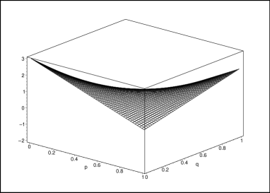
Figure 1: The payoff of player A versus strategy parameters $p$ and $q$ with initial state $|11\rangle$ in a $2\times 3$ matrix strategy game.

The payoff of player A with respect to $p$ and $q$ is plotted in Fig.1. The 3D-figure displays a shape of saddle, and the saddle-point is the Nash Equilibrium point. The precise value can be found by solving

$$\frac{\partial P_{A}}{\partial p} = \frac{13}{2}q-\frac{5}{2}=0$$ (14)

$$\frac{\partial P_{A}}{\partial q} = \frac{13}{2}p-5=0,$$

which give the Nash Equilibrium strategies at $p=\frac{10}{13}$, $q=\frac{5}{13}$. The corresponding payoff is $\frac{14}{13}$, and payoff for player $B$ is $-\frac{14}{13}$. If $a_{0}=0$, $a_{1}=1$ , then the payoff of player A is $0$ in Nash Equilibrium strategies, which is exactly the same as that in classical game. In these two cases, the initial state is a product states, a Nash equilibrium can be found. But it is not always equal to the classical counterpart.

It is interesting to point out that although in classical game Nash equilibrium always exist, it is not true in an arbitrarily designed quantum game such as this one. When entanglement is present in the initial state, the quantum game may have quite different properties compared with classical game. If we choose an entangled initial state, say let $a_{0}=a_{1}=\frac{1}{\sqrt{2}}$, no Nash Equilibrium point exists. This example clearly shows the difference between classical game and quantum game. When the initial state is a product, Nash equilibrium can be found, but the payoff may not be the same as that in the classical game.

Suppose both players have three distinct strategies, and the payoff matrix of player A is

$$\left[\begin{array}[]{cccc}&\left[1\right]&\left[2\right]&\left[3\right]\\ \left[1\right]&2&0&2\\ \left[2\right]&0&3&1\\ \left[3\right]&1&2&1\end{array}\right].$$ (15)

The classical Nash Equilibrium strategy is ($\frac{1}{3},0,\frac{2}{3}$) for player A, and $(\frac{1}{3},\frac{1}{3},\frac{1}{3})$ for player B. At Nash Equilibrium, the payoff of player A is $\frac{4}{3}$, and player B $-\frac{4}{3}$. In quantum game theory, we let the initial state $|\psi_{in}\rangle=a_{0}|11\rangle+a_{1}|22\rangle+a_{2}|33\rangle$ where $(\left|a_{0}\right|^{2}+\left|a_{1}\right|^{2}+\left|a_{2}\right|^{2}=1;a_{0},a_{1},a_{2}\geq 0)$. The players take the operators $U_{3A}=\sqrt{p}I-\sqrt{1-p}\exp(i\theta_{1})M$, $\theta_{1}=\arccos(\frac{1}{2}\sqrt{(1-p)/2p})$ and $U_{3B}=\sqrt{q}I-\sqrt{1-q}\exp(i\theta_{2})M$, where $\theta_{2}=\arccos(\frac{1}{2}\sqrt{(1-q)/2q})$, respectively. The payoff function of player $A$ is

$$P_{A} = \frac{5}{4}+(3a_{0}a_{2}+2a_{1}a_{2}+3a_{1}a_{0})\cos(\theta_{1}+\theta_{2})\sqrt{pq(1-p)(1-q)}$$

$$+(2a_{0}a_{2}+3a_{1}a_{2}+3a_{1}a_{0})\cos(\theta_{1}-\theta_{2})\sqrt{pq(1-p)(1-q)}$$

$$-(2a_{1}a_{0}+a_{0}a_{2}+2a_{1}a_{2})(1-p)\cos(\theta_{2})\sqrt{q(1-q)}$$

$$-(a_{1}a_{2}+2a_{0}a_{2}+3a_{1}a_{0})(1-q)\cos(\theta_{1})\sqrt{p(1-p)}+\frac{1}{4}a_{1}^{2}+\frac{1}{2}a_{0}^{2}$$

$$+(a_{1}a_{2}+\frac{1}{2}a_{1}a_{0}+\frac{3}{2}a_{0}a_{2})(1-pq)+(3a_{1}^{2}+\frac{9}{4}a_{0}^{2}-\frac{3}{4}a_{2}^{2})pq$$

$$+(\frac{1}{4}a_{2}^{2}-\frac{3}{2}a_{0}a_{2}-a_{1}a_{2}-a_{1}^{2}-\frac{3}{4}a_{0}^{2})(p+q)+\frac{1}{2}(a_{1}^{2}-a_{0}^{2})q.$$

If the initial state has no entanglement, say $a_{0}=1$, $a_{1}=a_{2}=0$, then the payoff function of player A is

$$P_{A}=\frac{9}{4}pq-\frac{3}{4}p-\frac{5}{4}q+\frac{7}{4}.$$ (17)

We have plotted the 3d-figure in Fig.2. We get a saddle point at $p=\frac{5}{9}$, $q=\frac{1}{3}$. The payoff function $P_{A}=\frac{4}{3}$ in Nash Equilibrium strategy which is the same as that of classical game. However, when $a_{0}=a_{1}=a_{2}=\frac{1}{\sqrt{3}}$, the payoff function is

$$P_{A} = \frac{1}{2}pq-\frac{4}{3}p-\frac{4}{3}q+\frac{5}{2}+\frac{16}{3}\cos\theta_{1}\cos\theta_{2}\sqrt{pq(1-p)(1-q)}$$

$$-\frac{5}{3}(1-p)\cos\theta_{2}\sqrt{q(1-q)}-2(1-q)\cos\theta_{1}\sqrt{p(1-p)}.$$

We have also plotted the 3-dimensional figure for the payoff of player A in Fig.3. We can not find any saddle point. In other word, the $Nash$ $Equilibrium$ strategy disappears in this quantum game. Likewise, when we let $a_{0}=a_{1}=\frac{1}{\sqrt{2}}$, $a_{2}=0$, the saddle does not exist either. All these show that the Nash Equilibrium strategy don’t always exist in quantum game in an entangled initial state.

In a general case when player A has $N$ strategies and player B has $M$ strategies, we assume the payoff function of player A is

$$A=\left[\begin{array}[]{ccccc}&\left[1\right]&\left[2\right]&\ldots&\left[M\right]\\ \left[1\right]&\alpha_{11}&\alpha_{12}&\ldots&\alpha_{1M}\\ \left[2\right]&\alpha_{21}&\alpha_{11}&\ldots&\alpha_{2M}\\ \ldots&\ldots&\ldots&\ldots&\ldots\\ \left[N\right]&\alpha_{N1}&\alpha_{N2}&\ldots&\alpha_{NM}\end{array}\right].$$ (19)

Generally, we use the initial state $|\psi_{in}\rangle=\sum\limits_{ijk}a_{k}|ij\rangle$, where $\sum\limits_{k}\left|a_{k}\right|^{2}=1$; $a_{k}\geq 0$. We define the $M$ matrices of player $A$ and player $B$.

$$M_{A(N\times N)}=\frac{1}{\sqrt{N-1}}\left[\begin{array}[]{cccc}0&1&\ldots&1\\ 1&0&\ldots&1\\ \ldots&1&\ldots&\ldots\\ 1&1&\ldots&0\end{array}\right],M_{B(M\times M)}=\frac{1}{\sqrt{M-1}}\left[\begin{array}[]{cccc}0&1&\ldots&1\\ 1&0&\ldots&1\\ \ldots&1&\ldots&\ldots\\ 1&1&\ldots&0\end{array}\right].$$ (20)

We see, if we write $|1\rangle=\left(1,0,\ldots 0\right)^{T}$, $|2\rangle=\left(0,1,\ldots 0\right)^{T}$,…$|n\rangle=\left(0,0,\ldots 1\right)^{T}$. Then we have $M_{A}|1\rangle\longrightarrow|2\rangle+|3\rangle+\ldots+|n\rangle$, …$M_{A}|n\rangle\longrightarrow|1\rangle+|2\rangle+\ldots+|n-1\rangle$. It will transform a basis state into the superposition of the rest of the basis states. We assume that in the game player $A$ take the unitary operator $\sqrt{p}I-\sqrt{1-p}\exp(i\theta_{A})M_{A}$, $\theta_{A}=\arccos(\frac{n-2}{2}\sqrt{\frac{1-p}{(n-1)p}})$ and player $B$ take the operator $\sqrt{q}I-\sqrt{1-q}\exp(i\theta_{B})M_{B}$, $\theta_{B}=\arccos(\frac{m-2}{2}\sqrt{\frac{1-p}{(m-1)p}})$. They can choose a specific value for parameter $p$ and $q$. After the operation the state vector becomes

$$|\psi_{out}\rangle=C_{11}|11\rangle+C_{12}|12\rangle+\ldots+C_{1m}|1m\rangle+C_{21}|21\rangle+\ldots+C_{nm}|nm\rangle,$$ (21)

where $\sum\limits_{i,j}^{n,m}\left|C_{ij}\right|^{2}=1$, and we let $x_{ij}=\left|C_{ij}\right|^{2}$. We write the probability matrix

$$X=\left[\begin{array}[]{cccc}x_{11}&x_{12}&\ldots&x_{1m}\\ x_{21}&x_{22}&\ldots&x_{2m}\\ \ldots&\ldots&\ldots&\ldots\\ x_{n1}&x_{n2}&\ldots&x_{nm}\end{array}\right].$$ (22)

From equations (20,21), we obtain

$$P_{A}(p,q)=Tr(XA^{T})=\sum\limits_{i,j}^{N,M}x_{ij}a_{ij}.$$ (23)

Now, we let

$$\frac{\partial P_{A}}{\partial p} = 0,$$ (24)

$$\frac{\partial P_{A}}{\partial q} = 0.$$

In term of the equation (24), we may obtain the saddle point $p_{0}$, $q_{0}$ and the payoff functions $P_{A}=P_{A}(p_{0},q_{0})$ and $P_{B}=-P_{A}(p_{0},q_{0})$ at the Nash Equilibrium point as well. It should be emphasized that Nash Equilibrium point does not always exist in the quantum game. Moreover, it is possible to have more than one saddle point in quantum game.

In this paper, we have studied a special multiple strategy quantum game. It is explicitly demonstrated that entanglement plays an important role in this quantum game, and it makes the quantum game different from that of classical game. In particular, it is found that when the initial state is entangled, Nash equilibrium does not always exist, in contrast to classical game. However, when the initial state is a product state, Nash equilibrium exists. This difference between quantum game and classical game is because we have set constraint on the allowed strategies of the two players. When the players are given then freedom to choose freely the pure strategies, Nash equilibrium always existslee ; suncp . However, for practical purpose, it is appealing to have a reasonable quantum game with a limited strategy space. As quantum game theory maybe applicable to many problems, a restricted strategy quantum game maybe occur, then one must be careful to examine the strategy set, especially when the initial state is entangled.

Finally, we thank Mr. Y. S. Li and Miss Liu Fang for help. This work is supported in part by China National Science Foundation, the Fok Ying Tung education foundation, the National Fundamental Research Program, Contract No. 001CB309308 and the Hang-Tian Science foundation.

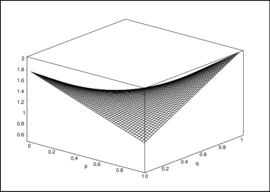
Figure 2: The payoff of player A versus strategy parameters $p$ and $q$ with initial state $|11\rangle$ in a $3\times 3$ matrix strategy game.

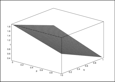
Figure 3: The payoff of player A versus strategy parameters $p$ and $q$ with an entangled initial state $\sqrt{1\over 3}(|11\rangle+|22\rangle+|33\rangle)$ in a $3\times 3$ matrix strategy game.

References

(1) J. Eisert,
M. Wilkens and M. Lewenstein, Phys. Rev. Lett.83,3077(1999)
(2) J.
Eisert, M. Wilkens, J. Mod. Opt.47, 2543(2000)
(3) S. C. Benjamin,
P. M. Hayden, Phys. Rev.A64,030301(2001)
(4) A. Iqbal, A.H. Toor, Phys.
Lett.A293,103 (2002)
(5) Y. J. Ma, G. L. Long, F. G. Deng, F. Li and S. X. Zhang, Phys. Lett.A, 301,117 (2002).
(6) J. F. Du, et al. Phys. Rev. Lett.88, 137902 (2002)
(7) L. Marinatto and T. Weber, Phys. Lett.A272, 291(2000)
(8) A. Iqbal and A. H. Toor, Phys. Lett.A280, 249 (2001)
(9) J. von Neumann, O. Morgenstern, Theory of Games and Economic Behaviour,
Princeton University Press; 3rd edition, 1953.
(10) C. F. Lee and N. F. Johnson, Lanl-eprint
quant-ph/0207012
(11) X. F. Liu and C. P. Sun, Lanl-eprint,
quant-ph/0212045