Measurement-based quantum computation on cluster states

Abstract

We give a detailed account of the one-way quantum computer, a scheme of quantum computation that consists entirely of one-qubit measurements on a particular class of entangled states, the cluster states. We prove its universality, describe why its underlying computational model is different from the network model of quantum computation and relate quantum algorithms to mathematical graphs. Further we investigate the scaling of required resources and give a number of examples for circuits of practical interest such as the circuit for quantum Fourier transformation and for the quantum adder. Finally, we describe computation with clusters of finite size.

I Introduction

Recently, we introduced the scheme of the one-way quantum computer ($\mbox{QC}_{\cal{C}}\;$) QCmeas . This scheme uses a given entangled state, the so-called cluster state BR , as its central physical resource. The entire quantum computation consists only of a sequence of one-qubit projective measurements on this entangled state. Thus it uses measurements as the central tool to drive a computation Nil97 - Nil . We called this scheme the “one-way quantum computer” since the entanglement in the cluster state is destroyed by the one-qubit measurements and therefore it can only be used once. To emphasize the importance of the cluster state for the scheme, we use the abbreviation $\mbox{QC}_{\cal{C}}\;$for “one-way quantum computer”.

The $\mbox{QC}_{\cal{C}}\;$is universal since any unitary quantum logic network can be simulated on it efficiently. The $\mbox{QC}_{\cal{C}}\;$can thus be explained as a simulator of quantum logic networks. However, the computational model that emerges for the $\mbox{QC}_{\cal{C}}\;$QCmodel makes no reference to the concept of unitary evolution and it shall be pointed out from the beginning that the network model does not provide the most suitable description for the $\mbox{QC}_{\cal{C}}$. Nevertheless, the network model is the most widely used form of describing a quantum computer and therefore the relation between the network model and the $\mbox{QC}_{\cal{C}}\;$must be clarified.

The purpose of this paper is threefold. First, it is to give the proof for universality of the $\mbox{QC}_{\cal{C}}$; second, to relate quantum algorithms to graphs; and third, to provide a number of examples for $\mbox{QC}_{\cal{C}}$-circuits which are characteristic and of practical interest.

In Section II we give the universality proof for the described scheme of computation in a complete and detailed form. The proof has already been presented to a large part in QCmeas . What was not contained in QCmeas was the explanation of why and how the gate simulations on the $\mbox{QC}_{\cal{C}}\;$work. This omission seemed in order since the implementation of the gates discussed there (CNOT and arbitrary rotations) require only small clusters such that the functioning of the gates can be easily verified in a computer simulation. For the examples of gates and sub-circuits given in Section IV this is no longer the case. Generally, we want an analytic explanation for the functioning of the gate simulations on the $\mbox{QC}_{\cal{C}}$. This explanation is given in Section II.6 and applied to the gates of a universal set in Section II.7 as well as to more complicated examples in Section IV.

In Section II.8 we discuss the spatial, temporal and operational resources required in $\mbox{QC}_{\cal{C}}$-computations in relation to the resources needed for the corresponding quantum logic networks. We find that overheads are at most polynomial. But there do not always need to be overheads. For example, as shown in Section II.9, all $\mbox{QC}_{\cal{C}}$-circuits in the Clifford group have unit logical depth.

In Section III we discuss non-network aspects of the $\mbox{QC}_{\cal{C}}$. In Section III.1 we state the reasons why the network model is not adequate to describe the $\mbox{QC}_{\cal{C}}\;$in every respect. The network model is abandoned and replaced by a more appropriate model QCmodel . This model is described very briefly.

In Section III.2 we relate algorithms to graphs. We show that from every algorithm its Clifford part can be removed. The required algorithm-specific non-universal quantum resource to run the remainder of the quantum algorithm on the $\mbox{QC}_{\cal{C}}\;$is then a graph state Schlingel1 . All that remains of the Clifford part is a mathematical graph specifying this graph state.

In Section IV we give examples of larger gates and sub-circuits which may be of practical relevance, among them the $\mbox{QC}_{\cal{C}}$-circuit for quantum Fourier transformation and for the $n$-qubit adder.

In Section V we discuss the $\mbox{QC}_{\cal{C}}\;$computations on finite (small) clusters and in the presence of decoherence. We describe a variant of the scheme consisting of repeated steps of (re-)entangling a cluster via the Ising interaction, alternating with rounds of one-qubit measurements. Using this modified scheme it is possible to split long computations such that they fit piecewise on a small cluster.

II Universality of quantum computation via one-qubit-measurements

In this section we prove that the $\mbox{QC}_{\cal{C}}\;$is a universal quantum computer. The technique to accomplish this is to show that any quantum logic network can be simulated efficiently on the $\mbox{QC}_{\cal{C}}$. Before we go into the details, let us state the general picture.

For the one-way quantum computer, the entire resource for the quantum computation is provided initially in the form of a specific entangled state –the cluster state BR – of a large number of qubits. Information is then written onto the cluster, processed, and read out from the cluster by one-particle measurements only. The entangled state of the cluster thereby serves as a universal “substrate” for any quantum computation. It provides in advance all entanglement that is involved in the subsequent quantum computation. Cluster states can be created efficiently in any system with a quantum Ising-type interaction (at very low temperatures) between two-state particles in a lattice configuration.

It is important to realize here that information processing is possible even though the result of every measurement in any direction of the Bloch sphere is completely random. The mathematical expression for the randomness of the measurement results is that the reduced density operator for each qubit in the cluster state is $\frac{1}{2}{\bf{1}}$. The individual measurement results are random but correlated, and these correlations enable quantum computation on the $\mbox{QC}_{\cal{C}}$.

For clarity, let us emphasize that in the scheme of the $\mbox{QC}_{\cal{C}}\;$we distinguish between cluster qubits on ${\cal{C}}$ which are measured in the process of computation, and the logical qubits. The logical qubits constitute the quantum information being processed while the cluster qubits in the initial cluster state form an entanglement resource. Measurements of their individual one-qubit state drive the computation.

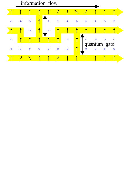
Figure 1: Simulation of a quantum logic network by measuring two-state particles on a lattice. Before the measurements the qubits are in the cluster state $|\phi\rangle_{\cal{C}}$ of (1). Circles $\odot$ symbolize measurements of $\sigma_{z}$, vertical arrows are measurements of $\sigma_{x}$, while tilted arrows refer to measurements in the x-y-plane.

To process quantum information with this cluster, it suffices to measure its particles in a certain order and in a certain basis, as depicted in Fig. 1. Quantum information is thereby propagated through the cluster and processed. Measurements of $\sigma_{z}$-observables effectively remove the respective lattice qubit from the cluster. Measurements in the $\sigma_{x}$- (and $\sigma_{y}$-) eigenbasis are used for “wires”, i.e. to propagate logical quantum bits through the cluster, and for the CNOT-gate between two logical qubits. Observables of the form $\cos(\varphi)\,\sigma_{x}\pm\sin(\varphi)\,\sigma_{y}$ are measured to realize arbitrary rotations of logical qubits. For these cluster qubits, the basis in which each of them is measured depends on the results of preceding measurements. This introduces a temporal order in which the measurements have to be performed. The processing is finished once all qubits except a last one on each wire have been measured. The remaining unmeasured qubits form the quantum register which is now ready to be read out. At this point, the results of previous measurements determine in which basis these “output” qubits need to be measured for the final readout, or if the readout measurements are in the $\sigma_{x}$-, $\sigma_{y}$- or $\sigma_{z}$-eigenbasis, how the readout measurements have to be interpreted. Without loss of generality, we assume in this paper that the readout measurements are performed in the $\sigma_{z}$-eigenbasis.

II.1 Cluster states and their quantum correlations

Cluster states are pure quantum states of two-level systems (qubits) located on a cluster ${\cal{C}}$. This cluster is a connected subset of a simple cubic lattice $\mathbb{Z}^{d}$ in $d\geq 1$ dimensions. The cluster states ${|\phi_{\{\kappa\}}\rangle}_{\cal{C}}$ obey the set of eigenvalue equations

$$K^{(a)}{|\phi_{\{\kappa\}}\rangle}_{\cal{C}}=(-1)^{\kappa_{a}}{|\phi_{\{\kappa\}}\rangle}_{\cal{C}},$$ (1)

with the correlation operators

$$K^{(a)}=\sigma_{x}^{(a)}\bigotimes\limits_{b\in\text{nbgh}(a)}\sigma_{z}^{(b)}.$$ (2)

Therein, $\{\kappa_{a}\in\{0,1\}|\,a\in{\cal{C}}\}$ is a set of binary parameters which specify the cluster state and $\text{nbgh}(a)$ is the set of all neighboring lattice sites of $a$. All states ${|\phi_{\{\kappa\}}\rangle}_{\cal{C}}$ are equally good for computation. A cluster state is completely specified by the eigenvalue equations (1). To see this, first note that two states $|\phi_{\{\kappa\}}\rangle_{\cal{C}}$ and $|\phi_{\{\tilde{\kappa}\}}\rangle_{\cal{C}}$ which obey a set of equations (1) but differ in at least one eigenvalue are orthogonal. This holds because if there exists an $a\in{\cal{C}}$ such that, say, $K^{(a)}|\phi_{\{\kappa\}}\rangle_{\cal{C}}=|\phi_{\{\kappa\}}\rangle_{\cal{C}}$ and $K^{(a)}|\phi_{\{\tilde{\kappa}\}}\rangle_{\cal{C}}=-|\phi_{\{\tilde{\kappa}\}}\rangle_{\cal{C}}$, then $\mbox{}_{\cal{C}}\langle\phi_{\{\tilde{\kappa}\}}|\phi_{\{\kappa\}}\rangle_{\cal{C}}=\mbox{}_{\cal{C}}\langle\phi_{\{\tilde{\kappa}\}}|K^{(a)}|\phi_{\{\kappa\}}\rangle_{\cal{C}}=-\mbox{}_{\cal{C}}\langle\phi_{\{\tilde{\kappa}\}}|\phi_{\{\kappa\}}\rangle_{\cal{C}}=0$. From the set of states which obey (1) with the eigenvalues specified by $\{\kappa\}$ a representative $|\phi_{\{\kappa\}}\rangle_{\cal{C}}$ is taken. There are $2^{|{\cal{C}}|}$ such classes of states, and hence $2^{|{\cal{C}}|}$ mutually orthogonal representatives $|\phi_{\{\kappa\}}\rangle_{\cal{C}}$. Therefore, the representative cluster states form a basis $\big{\{}{|\phi_{\{\kappa\}}\rangle_{\cal{C}}\,|\,\{\kappa\}\in\{0,1\}^{|{\cal{C}}|}}\big{\}}$ of the $|{\cal{C}}|$-qubit Hilbert space. To that end, let us now consider a state $|\phi^{\prime}_{\{\kappa\}_{0}}\rangle_{\cal{C}}$ that obeys (1) with the same $\{\kappa\}_{0}$ as $|\phi_{\{\kappa\}_{0}}\rangle_{\cal{C}}$, and expand it into the above basis. One finds $|\phi^{\prime}_{\{\kappa\}_{0}}\rangle_{\cal{C}}=\sum_{\{\kappa\}}\mbox{}_{\cal{C}}\langle\phi_{\{\kappa\}}|\phi^{\prime}_{\{\kappa\}_{0}}\rangle_{\cal{C}}\,|\phi_{\{\kappa\}}\rangle_{\cal{C}}=\mbox{}_{\cal{C}}\langle\phi_{\{\kappa\}_{0}}|\phi^{\prime}_{\{\kappa\}_{0}}\rangle_{\cal{C}}\,\,|\phi_{\{\kappa\}_{0}}\rangle_{\cal{C}}$. Hence, two states $|\phi^{\prime}_{\{\kappa\}_{0}}\rangle_{\cal{C}}$ and $|\phi_{\{\kappa\}_{0}}\rangle_{\cal{C}}$ which obey (1) with the same set ${\{\kappa\}}_{0}$ are the same modulo a possible global phase. Consequently, any method that creates a state obeying equations (1) with a specific set $\{\kappa_{a}|a\in{\cal{C}}\}$ creates the same state.

The eigenvalue equations (1) and the quantum correlations they imply are central for the described scheme of computation. Also, they represent a very compact way of characterizing the cluster states. To reflect this in the presentation, the discussion in this paper will be based entirely on these eigenvalue equations and we will never need to work out some cluster state in any specific basis. In fact, to write down a cluster state in its explicit form would be quite space-consuming since the minimum number of required terms scales exponentially with the number of qubits BR , and for computation we will be going to consider rather large cluster states. Nevertheless, for illustration we give a few examples of cluster states with a small number of qubits. The cluster states on a chain of 2, 3 and 4 qubits, fulfilling the eigenvalue equations (1) with all $\kappa_{a}=0$, are

$$\begin{array}[]{rcl}{|\phi\rangle}_{{\cal{C}}_{2}}&=&\displaystyle{\frac{1}{\sqrt{2}}\left({|0\rangle_{1}|+\rangle_{2}+|1\rangle_{1}|-\rangle_{2}}\right),}\\ {|\phi\rangle}_{{\cal{C}}_{3}}&=&\displaystyle{\frac{1}{\sqrt{2}}\left({|+\rangle_{1}|0\rangle_{2}|+\rangle_{3}+|-\rangle_{1}|1\rangle_{2}|-\rangle_{3}}\right),}\\ {|\phi\rangle}_{{\cal{C}}_{4}}&=&\displaystyle{\frac{1}{2}|+\rangle_{1}|0\rangle_{2}|+\rangle_{3}|0\rangle_{4}+\frac{1}{2}|+\rangle_{1}|0\rangle_{2}|-\rangle_{3}|1\rangle_{4},}\\ &&\displaystyle{+\frac{1}{2}|-\rangle_{1}|1\rangle_{2}|-\rangle_{3}|0\rangle_{4}+\frac{1}{2}|-\rangle_{1}|1\rangle_{2}|+\rangle_{3}|1\rangle_{4},}\end{array}$$ (3)

with the notations

$$\begin{array}[]{rcl}|0\rangle_{a}&:=&|0\rangle_{a,z}=\sigma_{z}^{(a)}|0\rangle_{a,z},\\ |1\rangle_{a}&:=&|1\rangle_{a,z}=-\sigma_{z}^{(a)}|1\rangle_{a,z},\\ |\pm\rangle_{a}&:=&\frac{1}{\sqrt{2}}(|0\rangle_{a}\pm|1\rangle_{a}).\end{array}$$ (4)

The state $|\phi\rangle_{{\cal{C}}_{2}}$ is local unitary equivalent to a Bell state and $|\phi\rangle_{{\cal{C}}_{3}}$ to the Greenberger-Horne-Zeilinger (GHZ) state. $|\phi\rangle_{{\cal{C}}_{4}}$ is not equivalent to a 4-particle GHZ state. In particular, the entanglement in $|\phi\rangle_{{\cal{C}}_{4}}$ cannot be destroyed by a single local operation BR .

Ways to create a cluster state in principle are to measure all the correlation operators $K^{(a)},\;a\in{\cal{C}}$ of (2) on an arbitrary $|{\cal{C}}|$-qubit state or to cool into the ground state of a Hamiltonian $H_{K}=-\hbar g\sum_{a\in{\cal{C}}}\kappa_{a}K^{(a)}$.

Another way –likely to be more suitable for realization in the lab– is as follows. First, a product state $|+\rangle_{\cal{C}}=\bigotimes_{a\in{\cal{C}}}|+\rangle_{a}$ is prepared. Second, the unitary transformation $S^{({\cal{C}})}$,

$$S^{({\cal{C}})}=\prod\limits_{a,b\in{\cal{C}}|b-a\in\gamma_{d}}S^{ab},$$ (5)

is applied to the state $|+\rangle$. Often we will write $S$ in short for $S^{({\cal{C}})}$. In (5), for the cases of dimension $d=1,2,3$, we have $\gamma_{1}=\{1\}$, $\gamma_{2}=\{(1,0)^{T},(0,1)^{T}\}$ and $\gamma_{3}=\{(1,0,0)^{T},(0,1,0)^{T},(0,0,1)^{T}\}$, and the two-qubit transformation $S^{ab}$ is such that the state $|1\rangle_{a}\otimes|1\rangle_{b}$ acquires a phase of $\pi$ under its action while the remaining states $|0\rangle_{a}\otimes|0\rangle_{b}$, $|0\rangle_{a}\otimes|1\rangle_{b}$ and $|1\rangle_{a}\otimes|0\rangle_{b}$ acquire no phase. Thus, $S^{ab}$ has the form

$$S^{ab}=\frac{1}{2}\left({\bf{1}}+\sigma_{z}^{(a)}+\sigma_{z}^{(b)}-\sigma_{z}^{(a)}\otimes\sigma_{z}^{(b)}\right).$$ (6)

The state $|+\rangle_{\cal{C}}$ obviously obeys the eigenvalue equations $\sigma_{x}^{(a)}|+\rangle_{\cal{C}}=|+\rangle_{\cal{C}}\;\forall a\in{\cal{C}}$ and thus the cluster state $|\phi\rangle_{\cal{C}}\;$ generated via $S$ obeys

$$|\phi\rangle_{\cal{C}}\;=S\sigma_{x}^{(a)}S^{\dagger}\,|\phi\rangle_{\cal{C}}\;,\;\;\forall a\in{\cal{C}}.$$ (7)

To obtain $S\sigma_{x}^{(a)}S^{\dagger}$, observe that

$$\begin{array}[]{rcl}S^{ab}\sigma_{x}^{(a)}{S^{ab}}^{\dagger}&=&\sigma_{x}^{(a)}\otimes\sigma_{z}^{(b)},\\ S^{ab}\sigma_{x}^{(b)}{S^{ab}}^{\dagger}&=&\sigma_{z}^{(a)}\otimes\sigma_{x}^{(b)},\end{array}$$ (8)

and

$$S^{ab}\sigma_{x}^{(c)}{S^{ab}}^{\dagger}=\sigma_{x}^{(c)},\;\;\forall c\in{\cal{C}}\backslash\{a,b\}.$$ (9)

Further, the Pauli phase flip operators $\sigma_{z}^{(d)}$ commute with all $S^{ab}$, i.e.

$$S^{ab}\sigma_{z}^{(d)}{S^{ab}}^{\dagger}=\sigma_{z}^{(d)},\;\;\forall d\in{\cal{C}}.$$ (10)

Now, from (8), (9) and (10) it follows that

$$S\sigma_{x}^{(a)}S^{\dagger}=\sigma_{x}^{(a)}\!\!\!\!\!\bigotimes\limits_{b\in\text{nbgh}(a)}\!\!\!\!\!\sigma_{z}^{(b)}.$$ (11)

Thus, the state $|\phi\rangle_{\cal{C}}\;$ generated from $|+\rangle_{\cal{C}}$ via the transformation $S$ as defined in (5) does indeed obey eigenvalue equations of form (1), with

$$\kappa_{a}=0,\;\,\,\forall\,a\in{\cal{C}}.$$ (12)

Note that all operations $S^{ab}$ in $S$ mutually commute and that they can therefore be carried out at the same time. Initial individual preparation of the cluster qubits in $|+\rangle_{a\in{\cal{C}}}$ can also be done in parallel. Thus, the creation of the cluster state is a two step process. The temporal resources to create the cluster state are constant in the size of the cluster.

If a cluster state is created as described above this leads to the specific set of eigenvalues in (1) specified by the parameters $\kappa_{a}$ in (12). As the eigenvalues are fixed in this case, we drop them in the notation for the cluster state $|\phi\rangle_{\cal{C}}\;$. Cluster states specified by different sets $\{\kappa_{a}\}$ can be obtained by applying Pauli phase flip operators $\sigma_{z}^{(a)}$. To see this, note that

$$\sigma_{z}^{(a)}K^{(b)}{\sigma_{z}^{(a)}}^{\dagger}=(-1)^{\delta_{a,b}}\,K^{(b)}.$$ (13)

Therefore,

$$\bigotimes\limits_{a\in{\cal{C}}}\left(\sigma_{z}^{(a)}\right)^{\Delta\kappa_{a}}\,\,|\phi_{\{\kappa_{a}\}}\rangle_{\cal{C}}=|\phi_{\{\kappa_{a}+\Delta\kappa_{a}\}}\rangle_{\cal{C}},$$ (14)

where the addition for the $\kappa_{a}$ is modulo 2.

The transformation $S$ defined in (5) is generated by the Hamiltonian

$$H=\hbar g\sum\limits_{a,b\in{\cal{C}}|b-a\in\gamma_{d}}\frac{1-\sigma_{z}^{(a)}}{2}\frac{1-\sigma_{z}^{(b)}}{2},$$ (15)

and $S$ is of the form

$$S=\exp\left(-i\pi\sum\limits_{a,b\in{\cal{C}}|b-a\in\gamma_{d}}\frac{1-\sigma_{z}^{(a)}}{2}\frac{1-\sigma_{z}^{(b)}}{2}\right).$$ (16)

Expanding the exponent in (16), one obtains

$$\begin{array}[]{rcl}S&=&\displaystyle{\left[\prod\limits_{a,b\in{\cal{C}}|b-a\in\gamma_{d}}\!\!\!\!\!\!\!e^{-i\frac{\pi}{4}}\exp\left(i\frac{\pi}{4}\sigma_{z}^{(a)}\right)\exp\left(i\frac{\pi}{4}\sigma_{z}^{(b)}\right)\right]}\\ &&\displaystyle{\times\exp\left(-i\frac{\pi}{4}\sum\limits_{a,b\in{\cal{C}}|b-a\in\gamma_{d}}\sigma_{z}^{(a)}\sigma_{z}^{(b)}\right)}.\end{array}$$ (17)

We find that the interaction part $H_{I}$ of the Hamiltonian $H$ generating $S$ is of Ising form,

$$H_{I}=\hbar\frac{g}{4}\sum_{a,b\in{\cal{C}}|b-a\in\gamma_{d}}\sigma_{z}^{(a)}\sigma_{z}^{(b)},$$ (18)

and, since the local part $H_{\mbox{\footnotesize{local}}}$ of the Hamiltonian commutes with the Ising Hamiltonian $H_{I}$, the interaction $S$ generated by $H$ is local unitary equivalent to the unitary transformation generated by a Ising Hamiltonian.

For matter of presentation, the interaction $S^{ab}$ in (6) and, correspondingly, the local part of the Hamiltonian $H$ in (15) has been chosen in such a way that the eigenvalue equations (1) take the particularly simple form with $\kappa_{a}=0$ for all $a\in{\cal{C}}$, irrespective of the shape of the cluster.

Concerning the creation of states that are useful as a resource for the $\mbox{QC}_{\cal{C}}$, i.e. cluster- or local unitary equivalent states, all systems with a tunable Ising interaction and a local $\sigma_{z}$-type Hamiltonian, i.e. with a Hamiltonian

$$H^{\prime}=\sum_{a\in{\cal{C}}}\Delta E_{a}\,\sigma_{z}^{(a)}+\hbar\frac{g(t)}{4}\sum_{a,b\in{\cal{C}}|b-a\in\gamma_{d}}\sigma_{z}^{(a)}\sigma_{z}^{(b)}$$ (19)

are suitable, provided the coupling $g(t)$ can be switched between zero and at least one nonzero value.

Even this condition can be relaxed. A permanent Ising interaction instead of a globally tunable one is sufficient, if the measurement process is much faster than the characteristic time scale for the Ising interaction, i.e. if the measurements are stroboscopic. If it takes the Ising interaction a time $T_{\text{Ising}}$ to create a cluster state $|\phi\rangle_{\cal{C}}\;$ from a product state $|+\rangle_{\cal{C}}$, then the Ising interaction acting for a time $2T_{\text{Ising}}$ performs the identity operation, $S^{({\cal{C}})}S^{({\cal{C}})}=1{\bf l}^{({\cal{C}})}$. Therefore, starting with a product state $|+\rangle_{\cal{C}}$ at time $t=0$ evolving under permanent Ising interaction, stroboscopic measurements may be performed at times $\left(2k+1\right)T_{\text{Ising}},\;k\in\mathbb{N}$.

Some basic notions of graph theory will later, in the universality proof, simplify the formulation of our specifications. Therefore let us, at this point, establish a connection between quantum states such as the cluster state of (1) and graphs. The treatment here follows that of Schlingel1 , adapted to our notation.

First let us recall the definition of a graph. A graph $G(V,E)$ is a set $V$ of vertices connected via edges $e$ from the set $E$. The information of which vertex $a\in V$ is connected to which other vertex $b\in V$ is contained in a symmetric $|V|\times|V|$ matrix $\Gamma$, the adjacency matrix. The matrix $\Gamma$ is such that $\Gamma_{ab}=1$ if two vertices $a$ and $b$ are connected via an edge $e\in E$, and $\Gamma_{ab}=0$ otherwise. We identify the cluster ${\cal{C}}$ with the vertices $V_{\cal{C}}$ of a graph, ${\cal{C}}=V_{\cal{C}}$, and in this way establish a connection to the notion introduced earlier.

To relate graphs to quantum mechanics, the vertices of a graph can be identified with local quantum systems, in this case qubits, and the edges with two-particle interactions Schlingel1 ,Rudolph , in the present case $\sigma_{z}\sigma_{z}$-interactions. If one initially prepares each individual qubit $a$ in the state ${(\sigma_{z}^{(a)})}^{\kappa_{a}}\,|+\rangle_{a}$ and subsequently switches on, for an appropriately chosen finite time span, the interaction

$$H_{G(V,E)}=\hbar g\sum_{(a,b)\in E}\frac{1-\sigma_{z}^{(a)}}{2}\frac{1-\sigma_{z}^{(b)}}{2},$$ (20)

with $(a,b)\in E$ denoting an edge between qubits $a$ and $b$, then one obtains quantum states that are graph code words as introduced in Schlingel1 . Henceforth we will refer to these graph code words as graph states and use them in a context different from coding. The graph states $|\phi\{\kappa\}\rangle_{G}$ are defined by a set of eigenvalue equations which read

$$\sigma_{x}^{(a)}\bigotimes_{b\in V}\left(\sigma_{z}^{(b)}\right)^{\Gamma_{ab}}|\phi\{\kappa\}\rangle_{G}={(-1)}^{\kappa_{a}}|\phi\{\kappa\}\rangle_{G},$$ (21)

with $\kappa_{a}\in\{0,1\}\;\forall\,a\in V$. Here we use $G$ instead of $V$ as an index for the state $|\phi\rangle$ as the set $E\subset V\times V$ of edges is now independent and no longer implicitly specified by $V$ as was the case in (1).

Note that cluster states (1) are a particular case of graph states (21). The graph $G({\cal{C}},E_{\cal{C}})$ which describes a cluster state is that of a square lattice in 2D and that of a simple cubic lattice in 3D, i.e. the set $E_{\cal{C}}$ of edges is given by

$$E_{\cal{C}}=\big{\{}(a,b)|\,a,b\in{\cal{C}},b\in\text{nbgh}(a)\big{\}}.$$ (22)

Let us at the end of this section mention how cluster states may be created in practice. One possibility is via cold controlled collisions in optical lattices, as described in BR . Cold atoms representing the qubits can be arranged on a two- or three dimensional lattice and state-dependent interaction phases may be acquired via cold collisions between neighboring atoms Jaksch or via tunneling Duan . For a suitable choice of the collision phases $\varphi$, $\varphi=\pi\;\mbox{mod}\,\,2\pi$, the state resulting from a product state $|+\rangle_{\cal{C}}$ after interaction is a cluster state obeying the eigenvalue equations (1), with the set $\{\kappa_{a},a\in{\cal{C}}\}$ specified by the filling pattern of the lattice.

II.2 A universal set of quantum gates

To provide something definite to discuss right from the beginning, we now give the procedures of how to realize a CNOT-gate and a general one-qubit rotation via one-qubit measurements on a cluster state. The explanation of why and how these gates work will be given in Section II.7.

(a)
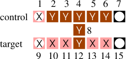
CNOT-gate
(b)	(c)
general rotation	$z$-rotation
(d)	(e)
Hadamard-gate	$\pi/2$-phase gate

Figure 2: Realization of elementary quantum gates on the $\mbox{QC}_{\cal{C}}$. Each square represents a lattice qubit. The squares in the extreme left column marked with white circles denote the input qubits, those in the right-most column denote the output qubits.

A CNOT-gate can be realized on a cluster state of 15 qubits, as shown in Fig. 2. All measurements can be performed simultaneously. The procedure to realize a CNOT-gate on a cluster with 15 qubits as displayed in Fig. 2 is

Procedure 1

Realization of a CNOT-gate acting on a two-qubit state $|\psi_{\text{in}}\rangle$.

1. Prepare the state
   $|\Psi_{\text{in}}\rangle_{{\cal{C}}_{15}}=|\psi_{\text{in}}\rangle_{1,9}\otimes\left(\bigotimes_{i\in{{\cal{C}}_{15}}\backslash\{1,9\}}|+\rangle_{i}\right)$.

2. Entangle the 15 qubits of the cluster ${\cal{C}}_{15}$ via the unitary operation $S^{({\cal{C}}_{15})}$.

3. Measure all qubits of ${\cal{C}}_{15}$ except for the output qubits 7, 15 (following the labeling in Fig. 2). The measurements can be performed simultaneously. Qubits 1, 9, 10, 11, 13, 14 are measured in the $\sigma_{x}$-eigenbasis and qubits 2-6, 8, 12 in the $\sigma_{y}$-eigenbasis.

Dependent on the measurement results, the following gate is thereby realized:

$$U^{\prime}_{CNOT}=U_{\Sigma,CNOT}\,CNOT(c,t).$$ (23)

Therein the byproduct operator $U_{\Sigma,CNOT}$ has the form

$$\begin{array}[]{rcl}U_{\Sigma,CNOT}&=&{\sigma_{x}^{(c)}}^{\gamma_{x}^{(c)}}{\sigma_{x}^{(t)}}^{\gamma_{x}^{(t)}}{\sigma_{z}^{(c)}}^{\gamma_{z}^{(c)}}{\sigma_{z}^{(t)}}^{\gamma_{z}^{(t)}},\;\mbox{with}\\ &\\ {\gamma_{x}^{(c)}}&=&{s}_{2}+{s}_{3}+{s}_{5}+{s}_{6}\\ {\gamma_{x}^{(t)}}&=&{s}_{2}+{s}_{3}+{s}_{8}+{s}_{10}+{s}_{12}+{s}_{14}\\ {\gamma_{z}^{(c)}}&=&{s}_{1}+{s}_{3}+{s}_{4}+{s}_{5}+{s}_{8}+{s}_{9}+{s}_{11}+1\\ {\gamma_{z}^{(t)}}&=&{s}_{9}+{s}_{11}+{s}_{13}.\end{array}$$ (24)

Therein, the ${s}_{i}$ represent the measurement outcomes $s_{i}$ on the qubits $i$. The expression (24) is modified if redundant cluster qubits are present and/or if the cluster state on which the CNOT gate is realized is specified by a set $\{\kappa_{a}\}$ different from (12), see Section II.3. This concludes the presentation of the CNOT gate, the proof of its functioning is given in Section II.7.

An arbitrary rotation $U_{Rot}\in SU(2)$ can be realized on a chain of 5 qubits. Consider a rotation in its Euler representation

$$U_{Rot}[\xi,\eta,\zeta]=U_{x}[\zeta]U_{z}[\eta]U_{x}[\xi],$$ (25)

where the rotations about the $x$- and $z$-axis are

$$\begin{array}[]{rcl}U_{x}[\alpha]&=&\displaystyle{\mbox{exp}\left(-i\alpha\frac{\sigma_{x}}{2}\right)\vspace{1.5mm}}\\ U_{z}[\alpha]&=&\displaystyle{\mbox{exp}\left(-i\alpha\frac{\sigma_{z}}{2}\right)}.\end{array}$$ (26)

Initially, the first qubit is prepared in some state $|\psi_{\mbox{\footnotesize{in}}}\rangle$, which is to be rotated, and the other qubits are prepared in $|+\rangle$. After the 5 qubits are entangled by the unitary transformation $S$, the state $|\psi_{\mbox{\footnotesize{in}}}\rangle$ can be rotated by measuring qubits 1 to 4. At the same time, the state is also swapped to site 5. The qubits $1\,..\,4$ are measured in appropriately chosen bases

$${\cal{B}}_{j}(\varphi_{j})=\left\{\frac{|0\rangle_{j}+e^{i\varphi_{j}}|1\rangle_{j}}{\sqrt{2}},\,\frac{|0\rangle_{j}-e^{i\varphi_{j}}|1\rangle_{j}}{\sqrt{2}}\right\},$$ (27)

whereby the measurement outcomes $s_{j}\in\{0,1\}$ for $j=1\,..\,4$ are obtained. Here, $s_{j}=0$ means that qubit $j$ is projected into the first state of ${\cal{B}}_{j}(\varphi_{j})$. In (27) the basis states of all possible measurement bases lie on the equator of the Bloch sphere, i.e. on the intersection of the Bloch sphere with the $x$-$y$-plane. Therefore, the measurement basis for qubit $j$ can be specified by a single parameter, the measurement angle $\varphi_{j}$. The measurement direction of qubit $j$ is the vector on the Bloch sphere which corresponds to the first state in the measurement basis ${\cal{B}}_{j}(\varphi_{j})$. Thus, the measurement angle $\varphi_{j}$ is the angle between the measurement direction at qubit $j$ and the positive $x$-axis. In summary, the procedure to realize an arbitrary rotation $U_{Rot}[\xi,\eta,\zeta]$, specified by its Euler angles $\xi,\eta,\zeta$, is this:

Procedure 2

Realization of general one-qubit rotations $U_{Rot}\in SU(2)$.

1. Prepare the state $|\Psi_{\mbox{\footnotesize{in}}}\rangle_{{\cal{C}}_{5}}=|\psi_{\mbox{\footnotesize{in}}}\rangle_{1}\otimes\left(\bigotimes_{i=2}^{5}|+\rangle_{i}\right)$.

2. Entangle the five qubits of the cluster ${\cal{C}}_{5}$ via the unitary operation $S^{({\cal{C}}_{5})}$.

3. Measure qubits 1 - 4 in the following order and basis

   $$\begin{array}[]{rl}\ref{Mea}.1&\mbox{measure qubit 1 in}\;{\cal{B}}_{1}(0)\\ \ref{Mea}.2&\mbox{measure qubit 2 in}\;{\cal{B}}_{2}\left(-\xi\,(-1)^{{s}_{1}}\right)\\ \ref{Mea}.3&\mbox{measure qubit 3 in}\;{\cal{B}}_{3}\left(-\eta\,(-1)^{{s}_{2}}\right)\\ \ref{Mea}.4&\mbox{measure qubit 4 in}\;{\cal{B}}_{4}\left(-\zeta\,(-1)^{{s}_{1}+{s}_{3}}\right)\end{array}$$ (28)

Via Procedure 2 the rotation $U_{Rot}^{\prime}$ is realized:

$$U_{Rot}^{\prime}[\xi,\eta,\zeta]=U_{\Sigma,Rot}\,U_{Rot}[\xi,\eta,\zeta].$$ (29)

Therein, the random byproduct operator has the form

$$U_{\Sigma,Rot}=\sigma_{x}^{{s}_{2}+{s}_{4}}\sigma_{z}^{{s}_{1}+{s}_{3}}.$$ (30)

It can be corrected for at the end of the computation, as will be explained in Section II.5.

There is a subgroup of rotations for which the realization procedure is somewhat simpler than Procedure 2. These rotations form the subgroup of local operations in the Clifford group. The Clifford group is the normalizer of the Pauli group.

Among these rotations are, for example, the Hadamard gate and the $\pi/2$-phase gate. These gates can be realized on a chain of 5 qubits in the following way:

Procedure 3

Realization of a Hadamard- and $\pi/2$-phase gate.

1. Prepare the state $|\Psi_{\mbox{\footnotesize{in}}}\rangle_{{\cal{C}}_{5}}=|\psi_{\mbox{\footnotesize{in}}}\rangle_{1}\otimes\left(\bigotimes_{i=2}^{5}|+\rangle_{i}\right)$.

2. Entangle the five qubits of the cluster ${\cal{C}}_{5}$ via the unitary operation $S^{({\cal{C}}_{5})}$.

3. Measure qubits 1 - 4. This can be done simultaneously. For the Hadamard gate, measure individually the observables $\sigma_{x}^{(1)}$, $\sigma_{y}^{(2)}$, $\sigma_{y}^{(3)}$, $\sigma_{y}^{(4)}$. For the $\pi/2$-phase gate measure $\sigma_{x}^{(1)}$, $\sigma_{x}^{(2)}$, $\sigma_{y}^{(3)}$, $\sigma_{x}^{(4)}$.

The difference with respect to Procedure 2 for general rotations is that in Procedure 3 no measurement bases need to be adjusted according to previous measurement results and therefore the measurements can all be performed at the same time.

As in the cases before, the Hadamard- and the $\pi/2$-phase gate are performed only modulo a subsequent byproduct operator which is determined by the random measurement outcomes ${s}_{k}$

$$\begin{array}[]{rcl}U_{\Sigma,H}&=&\sigma_{x}^{{s}_{1}+{s}_{3}+{s}_{4}}\,\sigma_{z}^{{s}_{2}+{s}_{3}}\\ U_{\Sigma,U_{z}(\pi/2)}&=&\sigma_{x}^{{s}_{2}+{s}_{4}}\,\sigma_{z}^{{s}_{1}+{s}_{2}+{s}_{3}+1}.\end{array}$$ (31)

Before we explain the functioning of the above gates, we would like to address the following questions: First,“How does one manage to occupy only those lattice sites with cluster qubits that are required for a particular circuit but leaves the remaining ones empty?”. The answer to this question is that redundant qubits will not have to be removed physically. It is sufficient to measure each of them in the $\sigma_{z}$-eigenbasis, as will be described in Section II.3.

Second, “How can the described procedures for gate simulation be concatenated such that they represent a measurement based simulation of an entire circuit?”. It seems at first sight that the described building blocks would only lead to a computational scheme consisting of repeated steps of entangling operations and measurements. This is not the case. As will be shown in Section II.4, the three procedures stated are precisely of such a form that the described measurement-based scheme of quantum computation can be decomposed into them.

The third question is: “How does one deal with the randomness of the measurement results that leads to the byproduct operators (24), (30) and (31)?”. The appearance of byproduct operators may suggest that there is a need for local correction operations to counteract these unwanted extra operators. However, there is neither a possibility for such counter rotations within the described model of quantum computation, nor is there a need. The scheme works with unit efficiency despite the randomness of the individual measurement results, as will be discussed in Section II.5.

II.3 Removing the redundant cluster qubits

A cluster state on a two-dimensional cluster of rectangular shape, say, is a resource that allows for any computation that fits on the cluster. If one realizes a certain quantum circuit on this cluster state, there will always be qubits on the cluster which are not needed for its realization. Such cluster qubits we call redundant for this particular circuit.

In the description of the $\mbox{QC}_{\cal{C}}\;$as a quantum logic network, the first step of each computation will be to remove these redundant cluster qubits. Fortunately, the situation is not such that we have to remove the qubits (or, more precisely, the carriers of the qubits) physically from the lattice. To make them ineffective to the realized circuit, it suffices to measure each of them in the $\sigma_{z}$-eigenbasis. In this way, one is left with an entangled quantum state on the cluster ${\cal{C}}_{N}$ of the unmeasured qubits and a product state on ${\cal{C}}\backslash{\cal{C}}_{N}$,

$${|\phi_{\{\kappa\}}\rangle}_{\cal{C}}\longrightarrow|Z\rangle_{{\cal{C}}\backslash{\cal{C}}_{N}}\otimes{|\phi_{\{\kappa^{\prime}\}}\rangle}_{{\cal{C}}_{N}},$$ (32)

with $|Z\rangle_{{\cal{C}}\backslash{\cal{C}}_{N}}=\left(\bigotimes_{i\in{\cal{C}}\backslash{\cal{C}}_{N}}|s_{i}\rangle_{i,z}\right)$ and $s_{i}$ the results of the $\sigma_{z}$-measurements. The resulting entangled state ${|\phi_{\{\kappa^{\prime}\}}\rangle}_{{\cal{C}}_{N}}$ on the sub-cluster ${\cal{C}}_{N}$ is again a cluster state obeying the set of equations (1). This can be seen as follows. First, by definition we have

$$\begin{array}[]{l}\displaystyle{|Z\rangle_{{\cal{C}}\backslash{\cal{C}}_{N}}\!\otimes\!{|\phi_{\{\kappa^{\prime}\}}\rangle}_{{\cal{C}}_{N}}}\!=\!\left(\bigotimes_{i\in{\cal{C}}\backslash{\cal{C}}_{N}}\frac{1+(-1)^{s_{i}}\sigma_{z}^{(i)}}{2}\right)\!{|\phi_{\{\kappa\}}\rangle}_{\cal{C}}.\end{array}$$ (33)

Using the eigenvalue equations (1), we now insert a correlation operator $K^{(a)}$ with $a\in{\cal{C}}_{N}$ into the r.h.s of (33) between the projector and the state, and obtain

$${|Z\rangle_{{\cal{C}}\backslash{\cal{C}}_{N}}\otimes{|\phi_{\{\kappa^{\prime}\}}\rangle}_{{\cal{C}}_{N}}}=(-1)^{\kappa_{a}^{\prime}}K^{\prime(a)}|Z\rangle_{{\cal{C}}\backslash{\cal{C}}_{N}}\otimes{|\phi_{\{\kappa^{\prime}\}}\rangle}_{{\cal{C}}_{N}},$$ (34)

with the correlation operators

$$K^{\prime(a)}=\sigma_{x}^{(a)}\!\!\!\!\bigotimes\limits_{c\in\mbox{\footnotesize{nbgh}}(a)\cap{\cal{C}}_{N}}\!\!\!\!\!\sigma_{z}^{(c)},$$ (35)

and the set $\{\kappa_{a}^{\prime}\}$ specifying the eigenvalues

$$\kappa^{\prime}_{a}=\left(\kappa_{a}+\sum\limits_{b\in\mbox{\footnotesize{nbgh}}(a)\cap({\cal{C}}\backslash{\cal{C}}_{N})}s_{b}\right)\;\mbox{mod}\,\,2.$$ (36)

As the new correlation operators $K^{\prime(a)}$ in (34) only act on the cluster qubits in ${\cal{C}}_{N}$, the states ${|\phi_{\{\kappa^{\prime}\}}\rangle}_{{\cal{C}}_{N}}$ again obey eigenvalue equations of type (1), i.e.

$$K^{\prime(a)}{|\phi_{\{\kappa^{\prime}\}}\rangle}_{{\cal{C}}_{N}}={(-1)}^{\kappa_{a}^{\prime}}{|\phi_{\{\kappa^{\prime}\}}\rangle}_{{\cal{C}}_{N}},\;\forall\,\,a\in{\cal{C}}_{N}.$$ (37)

There are $|{\cal{C}}_{N}|$ such eigenvalue equations for a state of $|{\cal{C}}_{N}|$ qubits. Thus, the state ${|\phi_{\{\kappa^{\prime}\}}\rangle}_{{\cal{C}}_{N}}$ is specified by (37) up to a global phase.

From (36) we find that the redundant qubits have some remaining influence on the process of computation. After they have been measured, the random measurement results enter into the eigenvalues that specify the residual cluster state ${|\phi_{\{\kappa^{\prime}\}}\rangle}_{{\cal{C}}_{N}}$ on the cluster ${\cal{C}}_{N}$. However, any cluster state ${|\phi_{\{\kappa^{\prime}\}}\rangle}_{{\cal{C}}_{N}}$ is equally good for computation as stated in Section II.1. From (14) it follows that

$${|\phi_{\{\kappa^{\prime}\}}\rangle}_{{\cal{C}}_{N}}=\bigotimes_{a\in{\cal{C}}_{N}}\left(\sigma_{z}^{(a)}\right)^{\kappa_{a}^{\prime}}|\phi\rangle_{{\cal{C}}_{N}}.$$ (38)

The Pauli phase flip operators that appear on the r.h.s. of equation (38) may be absorbed into the subsequent measurements. This allows us to adopt the following two rules in the further discussion

1. The redundant cluster qubits are discarded. We only consider the sub-cluster $${\cal{C}}_{N} \kappa^{\prime}_{a}=0 a\in{\cal{C}}_{N}$$. 2. We assume that for all . (39)

This reduction will make a number of expressions such as those for the byproduct operators more transparent and it will also simplify the remaining part of the universality proof.

II.4 Concatenation of gate simulations

A quantum circuit on the $\mbox{QC}_{\cal{C}}\;$is a spatial and temporal pattern of measurements on individual qubits which have previously been entangled to form a cluster state. To better understand its functioning we would like –as in the network model of quantum computation– to decompose the circuit into basic building blocks. These building blocks should be such that out of them any circuit can be assembled. In explaining the $\mbox{QC}_{\cal{C}}\;$in a network language, we can relate the building blocks of a quantum logic network –the quantum gates– to building blocks of $\mbox{QC}_{\cal{C}}$-circuits.

The fact that quantum gates can be combined to quantum logic networks is obvious. But the statement that, for a $\mbox{QC}_{\cal{C}}$-computation, measurement patterns which simulate gates can simply be patched together to give the measurement pattern for the whole circuit requires a proof. This proof is given next.

We begin by stating the general form of the procedures to realize gates and sub-circuits. The reason why these procedures work is explained in subsequent sections. To realize a gate $g$ on the $\mbox{QC}_{\cal{C}}\;$consider a cluster ${\cal{C}}(g)$. This cluster has an input section ${\cal{C}}_{I}(g)$, a body ${\cal{C}}_{M}(g)$ and an output section ${\cal{C}}_{O}(g)$, with

$$\begin{array}[]{c}\displaystyle{{\cal{C}}_{I}(g)\cup{\cal{C}}_{M}(g)\cup{\cal{C}}_{O}(g)={\cal{C}}(g)\vspace{1mm}}\\ \begin{array}[]{rcl}\displaystyle{{\cal{C}}_{I}(g)\cap{\cal{C}}_{M}(g)}&=&\emptyset\vspace{1mm}\\ \displaystyle{{\cal{C}}_{I}(g)\cap{\cal{C}}_{O}(g)}&=&\emptyset\vspace{1mm}\\ \displaystyle{{\cal{C}}_{M}(g)\cap{\cal{C}}_{O}(g)}&=&\emptyset.\end{array}\end{array}$$ (40)

The measurement bases of the qubits in ${\cal{C}}_{M}(g)$, the body of the gate $g$, encode $g$. The general scheme for procedures to realize a gate $g$ on a cluster ${\cal{C}}(g)$ is

Scheme 1

Simulation of the gate $g$ on ${\cal{C}}(g)$, acting on the input state $|\psi\rangle_{\text{in}}$.

1. Prepare the input state $|\psi_{\text{in}}\rangle$ on ${\cal{C}}_{I}(g)$ and the qubits in ${\cal{C}}_{M}(g)\cup{\cal{C}}_{O}(g)$ individually in the state $|+\rangle=|0\rangle_{x}$ such that the quantum state of all qubits in ${\cal{C}}(g)$ becomes

   $$|\Psi_{\text{in}}\rangle_{{\cal{C}}(g)}=|\psi_{\text{in}}\rangle_{{\cal{C}}_{I}(g)}\otimes\!\!\!\!\bigotimes_{k\in{\cal{C}}_{M}(g)\cup{\cal{C}}_{O}(g)}\!\!\!\!|+\rangle_{k}.$$ (41)

2. Entangle $|\Psi_{\text{in}}\rangle_{{\cal{C}}(g)}$ by the interaction

   $$S^{\left({\cal{C}}(g)\right)}=\prod_{a,b\in{\cal{C}}(g)|\,b-a\in\gamma_{d}}S^{ab},$$ (42)

   such that the resulting quantum state is $|\Psi_{\varepsilon}\rangle_{{\cal{C}}_{N}}=S^{\left({\cal{C}}(g)\right)}|\Psi_{\text{in}}\rangle_{{\cal{C}}(g)}$.

3. Measure the cluster qubits in ${\cal{C}}_{I}(g)\cup{\cal{C}}_{M}(g)$, i.e. choose measurement bases specified by $\vec{r}_{k}\in S^{2},\,\,k\in{\cal{C}}_{I}(g)\cup{\cal{C}}_{M}(g)$ and obtain the random measurement results $s_{k}$ such that the projector

   $$P^{({\cal{C}}_{I}(g)\cup{\cal{C}}_{M}(g))}=\!\!\!\!\bigotimes_{k\in{\cal{C}}_{I}(g)\cup{\cal{C}}_{M}(g)}\!\!\!\!\!\!\!\!\frac{1+{(-1)}^{s_{k}}\vec{r}_{k}\cdot\vec{\sigma}^{(k)}}{2}$$ (43)

   is applied. The resulting state is $|\Psi_{\text{out}}\rangle_{{\cal{C}}_{N}}=P^{({\cal{C}}_{I}(g)\cup{\cal{C}}_{M}(g))}|\Psi_{\varepsilon}\rangle_{{\cal{C}}_{N}}$.

Putting all three steps of Scheme 1 together, the relation between $|\Psi_{\text{in}}\rangle_{{\cal{C}}_{N}}$ and $|\Psi_{\text{out}}\rangle_{{\cal{C}}_{N}}$ is

$$|\Psi_{\text{out}}\rangle_{{\cal{C}}_{N}}=P^{({\cal{C}}_{I}(g)\cup{\cal{C}}_{M}(g))}\,S^{\left({\cal{C}}(g)\right)}\,|\Psi_{\text{in}}\rangle_{{\cal{C}}_{N}}.$$ (44)

As we will show later, the state $|\Psi_{\text{out}}\rangle_{{\cal{C}}_{N}}$ has the form

$$|\Psi_{\text{out}}\rangle_{{\cal{C}}_{N}}=\left(\bigotimes_{k\in{\cal{C}}_{I}(g)\cup{\cal{C}}_{M}(g)}\!\!\!\!\!\!\!|s_{k}\rangle_{k,\vec{r}_{k}}\right)\otimes|\psi_{\text{out}}\rangle_{{\cal{C}}_{O}(g)},$$ (45)

where $|s_{k}\rangle_{k,\vec{r}_{k}}$ denotes the state of the qubit $k$ after the observable $\vec{r}_{k}\cdot\vec{\sigma}^{(k)}$ has been measured and the measurement outcome was $s_{k}$, and

$$|\psi_{\text{out}}\rangle=U_{\Sigma,g}U_{g}|\psi_{\text{in}}\rangle.$$ (46)

Therein, $U_{g}$ is the desired unitary operation and $U_{\Sigma,g}$ an extra multi-local rotation that depends on the measurement results $\big{\{}s_{k}\,|\,\,k\in{\cal{C}}_{I}(g)\cup{\cal{C}}_{M}(g)\big{\}}$. The extra rotations $U_{\Sigma,g}$ are always in the Pauli group, i.e.

$$U_{\Sigma,g}=\bigotimes_{i=1}^{n}\left(\sigma_{x}^{[i]}\right)^{x_{i}}\left(\sigma_{z}^{[i]}\right)^{z_{i}}$$ (47)

modulo a possible global phase, and $n=|I|=|O|$. In (47) the $\sigma^{[i]}$ denote Pauli operators acting on the logical qubit $i$, not cluster qubit. The values $x_{i},z_{i}\in\{0,1\}$ are computed from the measurement outcomes $\big{\{}s_{k}\,|\,\,k\in{\cal{C}}_{I}(g)\cup{\cal{C}}_{M}(g)\big{\}}$.

We now have all prerequisites at hand to explain why measurement patterns of basic gates can be combined to form the measurement pattern of the whole circuit which is obtained by combining the gates. The scheme of quantum computation with the $\mbox{QC}_{\cal{C}}\;$consists of a single entangling operation which creates the resource cluster state and, subsequently, of a series of one-qubit measurements on that state. We want to view the measurement pattern of a quantum circuit as being composed of basic blocks from whose function the function of the whole circuit can be deduced. To do so, we will explain computation on the $\mbox{QC}_{\cal{C}}\;$as a sequential process of performing the circuit gate by gate. Then we have to demonstrate that the computational scheme as it is practically carried out, i.e. entangle once and afterwards only measure, and the sequential scheme that we use to explain the functioning of the circuit are mathematically equivalent.

The sequential scheme is this. Consider a circuit $U=\prod_{i=1}^{|{\cal{N}}|}U_{g_{i}}$ that consists of a succession of gates $g_{1},..,g_{|{\cal{N}}|}\in{\cal{N}}$ applied to some input state $|\psi_{\text{in}}\rangle$, leading to an output state $|\psi_{\text{out}}\rangle=U|\psi_{\text{in}}\rangle$ which is then measured. ${\cal{N}}$ denotes the network, i.e. the set of gates plus a description of their relation. For simplicity let us first assume that each gate $g_{i}$ acts on all of the logical qubits. Subsequently we will drop this assumption.

First, a quantum state $|\psi_{\text{in}}\rangle_{I}\otimes|+\rangle_{{\cal{C}}_{N}\backslash I}$ is prepared. Then each gate, one after another, is realized on a sub-cluster ${\cal{C}}(g)\subset{\cal{C}}_{N}$ according to Scheme 1. Finally, the output is measured as usual.

In the step of carrying out the gate $g_{i}$ the state of the quantum register is, besides being processed, also teleported from ${\cal{C}}_{I}(g_{i})={\cal{C}}_{O}(g_{i-1})$ to ${\cal{C}}_{O}(g_{i})={\cal{C}}_{I}(g_{i+1})$. In this way, by carrying out the gate $g_{i}$ the input for the successor gate $g_{i+1}$ is provided. To proceed with the realization of gate $g_{i+1}$, in accordance with Scheme 1, the sub-cluster ${\cal{C}}(g_{i+1})$ is entangled via $S^{({\cal{C}}(g_{i+1}))}$and subsequently the cluster qubits in ${\cal{C}}_{I}(g_{i+1})\cup{\cal{C}}_{M}(g_{i+1})$ are measured. This completes the realization of gate $g_{i+1}$ and at the same time writes the input for $g_{i+2}$, and so on.

The reason why the sequential scheme just described is equivalent to the entangle-once-and-then-only-measure scheme is the following. The entanglement operations at the various stages of the sequential scheme commute with all the measurements carried out earlier. This holds because both operations, entangling operation and earlier measurement, act on different particles. Thus, the operations may be reordered in such a way that in a first step all entangling operations $S^{({\cal{C}}(g_{i}))}$ act on the initial state and afterwards all the measurements are performed.

The exchange of the order of the one-particle measurements and the two-particle Ising interactions is shown in Fig. 3 for a 1D cluster. In one dimension the decomposition of a cluster into sub-clusters, as displayed in Fig. 3, is clear. However, the interesting cases for $\mbox{QC}_{\cal{C}}$-computations are clusters in 2D and 3D; and there we must state more precisely what “decomposition of a cluster into sub-clusters” means. The use of basic notions from graph theory will prove helpful for this purpose.

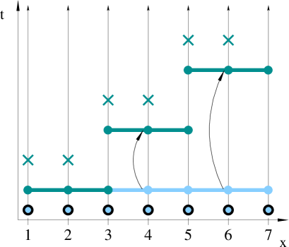
Figure 3: Here the exchange of the order of the measurements and the entanglement operations is shown. The crosses “$\times$” denote the one-qubit measurements and the horizontal lines between adjacent cluster qubits denote the unitary transformations $S^{a,a+1}$.

To decompose a cluster into sub-clusters means in more precise terms to decompose the associated graph $G({\cal{C}}_{N},E_{{\cal{C}}_{N}})$ into subgraphs. That is, we have to decompose both the vertices and the edges of the graph. Each vertex $a\in{\cal{C}}_{N}$ has to belong to a subset ${\cal{C}}(g_{i})$, where

$${\cal{C}}_{N}=\bigcup_{i=1}^{|{\cal{N}}|}{\cal{C}}(g_{i}),$$ (48)

and the sets ${\cal{C}}(g_{i})$ of vertices corresponding to the gates $g_{i}$ may overlap on their input- and output vertices.

Correspondingly, the set $E_{{\cal{C}}_{N}}$ of edges, defined in the same way as $E_{\cal{C}}$ in (22), is decomposed into subsets

$$E_{{\cal{C}}_{N}}=\bigcup_{i=1}^{|{\cal{N}}|}E(g_{i}),$$ (49)

but the subsets $E(g_{i})$ of edges are not allowed to overlap,

$$\forall i,j=1\,..\,|{\cal{N}}|,i\neq j:\;E(g_{i})\cap E(g_{j})=\emptyset.$$ (50)

The rules for the decomposition of edges (49) and (50) are, as we shall see, central for the universality proof.

Further, for the decomposition to be useful, the subsets ${\cal{C}}(g_{i})$ and $E(g_{i})$ must fulfill a number of constraints. The first of these is that each pair $({\cal{C}}(g_{i}),E(g_{i}))$ is again a graph, $G({\cal{C}}(g_{i}),E(g_{i}))$. This requires, in particular, that the endpoints of all the edges in $E(g_{i})$ are in ${\cal{C}}(g_{i})$,

$$\forall i=1,..,|{\cal{N}}|:E(g_{i})\subset{\cal{C}}(g_{i})\times{\cal{C}}(g_{i}).$$ (51)

For details on the graph decomposition, in particular for conditions on the subgraphs imposed to guarantee (49) and (50) see Appendix A.

Now consider the concatenation $g_{2}\circ g_{1}$ of the two gates $g_{1}$, realized on a cluster ${\cal{C}}(g_{1})$, and $g_{2}$, realized on a cluster ${\cal{C}}(g_{2})$, each of them by a procedure according to scheme 1. The composite circuit $g=g_{2}\circ g_{1}$ is realized on the cluster

$${\cal{C}}(g)={\cal{C}}(g_{1})\cup{\cal{C}}(g_{2}),$$ (52)

with

$$\begin{array}[]{rcl}\displaystyle{{\cal{C}}_{I}(g)}&=&\displaystyle{{\cal{C}}_{I}(g_{1})\cup\left({\cal{C}}_{I}(g_{2})\backslash{\cal{C}}_{O}(g_{1})\right)\vspace{0.1cm}}\\ \displaystyle{{\cal{C}}_{O}(g)}&=&\displaystyle{{\cal{C}}_{O}(g_{2})\cup\left({\cal{C}}_{O}(g_{1})\backslash{\cal{C}}_{I}(g_{2})\right)}.\end{array}$$ (53)

Now, the procedure to perform the two gates $g_{1}$, $g_{2}$ sequentially is

1. Prepare the state $|\Psi_{\text{in}}\rangle_{{\cal{C}}(g)}=|\psi_{\text{in}}\rangle_{{\cal{C}}_{I}(g)}\otimes|+\rangle_{{\cal{C}}(g)\backslash{{\cal{C}}_{I}(g)}}$.

2. Entangle the qubits on the sub-cluster ${\cal{C}}(g_{1})$ via

   $$S_{1}:=S^{({\cal{C}}(g_{1}))}=\prod_{a,b\in{\cal{C}}(g_{1})|\,b-a\in\gamma_{d}}\!\!\!\!S^{ab}.$$ (54)

3. Measure the qubits in ${\cal{C}}_{I}(g_{1})\cup{\cal{C}}_{M}(g_{1})$, resulting in the projector $P_{{\cal{C}}_{I}(g_{1})\cup{\cal{C}}_{M}(g_{1})}=:P_{1}$,

   $$P_{1}=\bigotimes_{k\in{\cal{C}}_{I}(g_{1})\cup{\cal{C}}_{M}(g_{1})}\!\!\!\!\!\!\frac{1+(-1)^{s_{k}}\vec{r}_{k}\cdot\vec{\sigma}^{(k)}}{2}.$$ (55)

   Therein $s_{k}$ is the outcome of the measurement of qubit $k$ and $\vec{r}_{k}$ the respective measurement direction.

4. Entangle the qubits on the sub-cluster ${\cal{C}}(g_{2})$ via

   $$S_{2}:=S^{({\cal{C}}(g_{2}))}=\prod_{a,b\in{\cal{C}}(g_{2})|\,b-a\in\gamma_{d}}\!\!\!\!S^{ab}.$$ (56)

5. Measure the qubits in ${\cal{C}}_{I}(g_{2})\cup{\cal{C}}_{M}(g_{2})$, resulting in the projector $P_{{\cal{C}}_{I}(g_{2})\cup{\cal{C}}_{M}(g_{2})}=:P_{2}$,

   $$P_{2}=\bigotimes_{k\in{\cal{C}}_{I}(g_{2})\cup{\cal{C}}_{M}(g_{2})}\!\!\!\!\!\!\frac{1+(-1)^{s_{k}}\vec{r}_{k}\cdot\vec{\sigma}^{(k)}}{2}.$$ (57)

The procedure results in an output state

$$|\Psi_{\text{out}}\rangle_{{\cal{C}}(g)}=P_{2}\,S_{2}\,P_{1}\,S_{1}|\Psi_{\text{in}}\rangle_{{\cal{C}}(g)}$$ (58)

that has the form

$$|\Psi_{\text{out}}\rangle_{{\cal{C}}(g)}=\left(\bigotimes_{{\cal{C}}_{I}(g)\cup{\cal{C}}_{M}(g)}\!\!\!\!\!|s_{k}\rangle_{k,\vec{r}_{k}}\right)\otimes|\psi_{\text{out}}\rangle_{{\cal{C}}_{O}(g)},$$ (59)

with

$$|\psi_{\text{out}}\rangle=U_{\Sigma,g_{2}}\,U_{g_{2}}U_{\Sigma,g_{1}}\,U_{g_{1}}|\psi_{\text{in}}\rangle,$$ (60)

according to (46).

As will be shown next, the above procedure is equivalent to a procedure of Scheme 1 applied to the cluster ${\cal{C}}(g)={\cal{C}}(g_{1})\cup{\cal{C}}(g_{2})$, i.e. when, first, all qubits in ${\cal{C}}(g)$ are entangled and, second, all but the output qubits of ${\cal{C}}_{O}(g)$ are measured.

The procedure according to Scheme 1 yields the state

$$|\Psi^{\prime}_{\text{out}}\rangle_{{\cal{C}}(g)}=P^{({\cal{C}}_{I}(g)\cup{\cal{C}}_{M}(g))}\,S^{({\cal{C}}(g))}\,|\Psi_{\text{in}}\rangle_{{\cal{C}}(g)},$$ (61)

and we now have to show that the output states $|\Psi_{\text{out}}\rangle_{{\cal{C}}(g)}$ in (58) and $|\Psi^{\prime}_{\text{out}}\rangle_{{\cal{C}}(g)}$ in (61) are the same for all input states $|\Psi_{\text{in}}\rangle_{{\cal{C}}(g)}$.

First note that the operations $P_{1}$ and $S_{2}$ commute since they act on different particles. $P_{1}$ acts on the qubits in ${\cal{C}}_{I}(g_{1})\cup{\cal{C}}_{M}(g_{1})$ while $S_{2}$ acts on ${\cal{C}}(g_{2})$. The sub-clusters associated with the gates may overlap only via their input- and output qubits. This is intuitively clear, and also follows from the decomposition constraint (187). As the gate $g_{1}$ is applied before $g_{2}$, of ${\cal{C}}(g_{1})$ only the qubits in ${\cal{C}}_{O}(g_{1})$ may overlap with the qubits in ${\cal{C}}_{I}(g_{2})$. Thus, $({\cal{C}}_{I}(g_{1})\cup{\cal{C}}_{M}(g_{1}))\cap{\cal{C}}(g_{2})=\emptyset$. Therefore

$$P_{2}\,S_{2}\,P_{1}\,S_{1}=P_{2}\,P_{1}\,S_{2}\,S_{1}.$$ (62)

Now note that as a direct consequence of (53) the union of the input- and body section of the composite gate $g$ on the cluster ${\cal{C}}(g)$ are made up by the union of the input- and body sections of the two individual gates $g_{1}$ and $g_{2}$, i.e.

$${\cal{C}}_{I}(g_{1})\cup{\cal{C}}_{M}(g_{1})\cup{\cal{C}}_{I}(g_{2})\cup{\cal{C}}_{M}(g_{2})={\cal{C}}_{I}(g)\cup{\cal{C}}_{M}(g).$$ (63)

Further, from the decomposition constraint (187) and from the fact that $g_{1}$ is applied before $g_{2}$ it follows that the input- and body sections of gates $g_{1}$ and $g_{2}$ do not intersect,

$$\left({\cal{C}}_{I}(g_{1})\cup{\cal{C}}_{M}(g_{1})\right)\cap\left({\cal{C}}_{I}(g_{2})\cup{\cal{C}}_{M}(g_{2})\right)=\emptyset.$$ (64)

Therefore,

$$\begin{array}[]{rcl}P_{2}\,P_{1}&=&\displaystyle{\bigotimes\limits_{{\cal{C}}_{I}(g_{2})\cup{\cal{C}}_{M}(g_{2})}\!\!\!\!\!\!\!\frac{1+(-1)^{s_{k}}\vec{r}_{k}\cdot\vec{\sigma}^{(k)}}{2}}\\ &&\mbox{ }\;\;\;\;\;\displaystyle{\bigotimes\limits_{{\cal{C}}_{I}(g_{1})\cup{\cal{C}}_{M}(g_{1})}\!\!\!\!\!\!\!\frac{1+(-1)^{s_{k}}\vec{r}_{k}\cdot\vec{\sigma}^{(k)}}{2}}\\ &=&\displaystyle{\bigotimes\limits_{{\cal{C}}_{I}(g)\cup{\cal{C}}_{M}(g)}\!\!\!\!\!\!\!\frac{1+(-1)^{s_{k}}\vec{r}_{k}\cdot\vec{\sigma}^{(k)}}{2}}\\ &=&\displaystyle{P^{({\cal{C}}_{I}(g)\cup{\cal{C}}_{M}(g))},}\end{array}$$ (65)

where the second line holds by (63) and (64). We find that measurement patterns corresponding to the projections $P_{1}$ and $P_{2}$ can be patched together to form the measurement pattern on the cluster ${\cal{C}}(g)$.

The same holds for the entangling operations. The entangling operation $S_{1}$ on ${\cal{C}}(g_{1})$ and $S_{2}$ on ${\cal{C}}(g_{2})$ combined give the entangling operation $S^{({\cal{C}}(g))}$ on ${\cal{C}}(g)$,

$$S_{2}\,S_{1}=S^{({\cal{C}}(g))},$$ (66)

because of the central rule (50).

Inserting (65) and (66) into (62) yields

$$P_{2}\,S_{2}\,P_{1}\,S_{1}=P^{({\cal{C}}_{I}(g)\cup{\cal{C}}_{M}(g))}\,S^{({\cal{C}}(g))},$$ (67)

and therefore, if we compare (58) and (61) we find that $|\Psi_{\text{out}}\rangle_{{\cal{C}}(g)}$, the output state of the sequential realization of the two gates $g_{1}$ and $g_{2}$, and $|\Psi^{\prime}_{\text{out}}\rangle_{{\cal{C}}(g)}$, the output state of the standard procedure applied to the composite circuit, are indeed the same for all inputs $|\Psi_{\text{in}}\rangle_{{\cal{C}}(g)}$. Thus both realizations, the sequential and the non-sequential, are equivalent.

This composition can be iterated so that the entire circuit can be realized via the standard procedure of Scheme 1. The measurement pattern of the circuit is thereby obtained by patching together the measurement patterns of the gates the circuit is composed of.

From (60) it follows that the quantum input $|\psi_{\text{in}}\rangle$ and the quantum output $|\psi_{\text{out}}\rangle$ of the unitary evolution are related via

$$|\psi_{\text{out}}\rangle=\left(\prod_{i=1}^{|{\cal{N}}|}U_{\Sigma,g_{i}}\,U_{g_{i}}\right)|\psi_{\text{in}}\rangle.$$ (68)

The random but known byproduct operators $U_{\Sigma,g_{i}}$ that appear in (68) are dealt with in Section II.5. The gates $g_{i}\in{\cal{N}}$ are labeled corresponding to the order of their action.

Now, we want to specify to the case where the quantum input is known and where the quantum output is measured. This is the situation which interests us most in this paper. Examples of such a situation are Shor’s factoring algorithm and Grover’s search algorithm. In both cases, the quantum input is $|\psi_{\text{in}}\rangle=\bigotimes_{i=1}^{n}|+\rangle_{i}$.

Let us denote the input section of the whole cluster ${\cal{C}}$, comprising the input qubits of the network simulation, as $I$; and the output section, comprising the qubits of the readout quantum register, as $O$. As long as the quantum input is known it is sufficient to consider the state $|+\rangle_{I}=\bigotimes_{i\in I}|+\rangle_{i}$. For different but known input states $|\psi_{\text{in}}\rangle_{I}$ one can always find a transformation $U_{\text{in}}$ such that $|\psi_{\text{in}}\rangle_{I}=U_{\text{in}}|+\rangle_{I}$ and instead of realizing some unitary transformation $U$ on $|\psi_{\text{in}}\rangle_{I}$ one realizes $U\,U_{\text{in}}$ on $|+\rangle_{I}$.

Preparing an input state $|+\rangle_{I}$ and entangling it via $S^{({\cal{C}})}$ is the same as creating a cluster state $|\phi\rangle_{\cal{C}}$, $S^{({\cal{C}})}\,|+\rangle_{I}\otimes|+\rangle_{{\cal{C}}\backslash I}=S^{({\cal{C}})}\,|+\rangle_{\cal{C}}=|\phi\rangle_{\cal{C}}\;$. This holds because the state $S^{({\cal{C}})}\,|+\rangle_{\cal{C}}$ obeys the eigenvalue equations (1) and, as we have stated earlier, these eigenvalue equations determine the state completely. Thus the created state is a cluster state $|\phi\rangle_{\cal{C}}\;$ that could as well have been prepared by any other means.

Once the quantum output is read then all cluster qubits have been measured. Therefore, the entire procedure of realizing a quantum computation on the $\mbox{QC}_{\cal{C}}\;$amounts to

Scheme 2

Performing a computation on the $\mbox{QC}_{\cal{C}}$.

1. Prepare a cluster state ${|\phi_{\{\kappa\}}\rangle}_{\cal{C}}$ of sufficient size.

2. Perform a sequence of measurements on ${|\phi_{\{\kappa\}}\rangle}_{\cal{C}}$ and obtain the result of the computation from all the measurement outcomes.

The link between the network model and the $\mbox{QC}_{\cal{C}}\;$is established by Scheme 1. The elementary constituents of the quantum logic network are mapped onto the corresponding basic blocks of the $\mbox{QC}_{\cal{C}}$. In this way, Scheme 1 helps to understand why the $\mbox{QC}_{\cal{C}}\;$works.

However, a $\mbox{QC}_{\cal{C}}$-computation is more appropriately described by Scheme 2 than by Scheme 1. Scheme 2 does not use the notion of quantum gates, but only of a spatial and temporal measurement pattern. Once universality of the $\mbox{QC}_{\cal{C}}\;$is established, to demonstrate the functioning of specific $\mbox{QC}_{\cal{C}}$-algorithms one would prefer decomposing a measurement pattern directly into sub-patterns rather than decomposing a network simulation into simulations of gates. A tool for the direct approach is provided by Theorem 1 in Section II.6.

II.5 Randomness of the measurement results

We will now show that the described scheme of quantum computation with the $\mbox{QC}_{\cal{C}}\;$works with unit efficiency despite the randomness of the individual measurement results.

First note that a byproduct operator $U_{\Sigma}$ that acts after the final unitary gate $U_{g_{|{\cal{N}}|}}$ does not jeopardize the scheme. Its only effect is that the results of the readout measurements have to be reinterpreted. The byproduct operator $U_{\Sigma}$ that acts upon the logical output qubits $1\,..\,n$ has the form

$$U_{\Sigma}=\prod\limits_{i=1}^{n}\,\,{\left(\sigma_{x}^{[i]}\right)}^{x_{i}}{\left(\sigma_{z}^{[i]}\right)}^{z_{i}},$$ (69)

where $x_{i},z_{i}\in\{0,1\}$ for $1\leq i\leq n$. Let the qubits on the cluster which are left unmeasured be labeled in the same way as the readout qubits of the quantum logic network.

The qubits on the cluster which take the role of the readout qubits are, at this point, in a state $U_{\Sigma}|\mbox{out}\rangle$, where $|\mbox{out}\rangle$ is the output state of the corresponding quantum logic network. The computation is completed by measuring each qubit in the $\sigma_{z}$-eigenbasis, thereby obtaining the measurement results $\{s_{i}^{\prime}\}$, say. In the $\mbox{QC}_{\cal{C}}$-scheme, one measures the state $U_{\Sigma}|\mbox{out}\rangle$ directly, whereby outcomes $\{s_{i}\}$ are obtained and the readout qubits are projected into the state $|{\cal{M}}\rangle=\prod_{i=1}^{n}\frac{1+{(-1)}^{s_{i}}\sigma_{z}^{(i)}}{2}\,\,U_{\Sigma}|\mbox{out}\rangle$. Depending on the byproduct operator $U_{\Sigma}$, the set of measurement results $\{s\}$ in general has a different interpretation from what the network readout $\{s_{i}^{\prime}\}$ would have. The measurement basis is the same. From (69) one obtains

$$\begin{array}[]{rcl}\displaystyle{|{\cal{M}}\rangle}&=&\displaystyle{\prod_{i=1}^{n}\frac{1+{(-1)}^{s_{i}}\sigma_{z}^{(i)}}{2}\,U_{\Sigma}|\mbox{out}\rangle\vspace*{0.1cm}}\\ &=&\displaystyle{U_{\Sigma}\left(U_{\Sigma}^{\dagger}\,\prod_{i=1}^{n}\frac{1+{(-1)}^{s_{i}}\sigma_{z}^{(i)}}{2}U_{\Sigma}\right)|\mbox{out}\rangle\vspace{0.1cm}}\\ &=&\displaystyle{U_{\Sigma}\,\prod_{i=1}^{n}\frac{1+{(-1)}^{s_{i}+x_{i}}\sigma_{z}^{(i)}}{2}|\mbox{out}\rangle}\end{array}$$ (70)

From (70) we see that a $\sigma_{z}$-measurement on the state $U_{\Sigma}\,|\mbox{out}\rangle$ with results $\{s\}$ represents the same algorithmic output as a $\sigma_{z}$-measurement of the state $|\mbox{out}\rangle$ with the results $\{s_{i}^{\prime}\}$, where the sets $\{s\}$ and $\{s_{i}^{\prime}\}$ are related by

$$s_{i}^{\prime}\equiv s_{i}+x_{i}\;\mbox{mod}\,\,2.$$ (71)

The set $\{s_{i}^{\prime}\}$ represents the result of the computation. It can be calculated from the results $\{s_{i}\}$ of the $\sigma_{z}$-measurements on the “readout” cluster qubits, and the values $\{x_{i}\}$ which are determined by the byproduct operator $U_{\Sigma}$.

Thus we find that one can cope with the randomness of the measurement results provided the byproduct operators $U_{\Sigma,g_{i}}$ in (68) can be propagated forward through the subsequent gates such that they act on the cluster qubits representing the output register. This can be done. To propagate the byproduct operators we use the propagation relations

$$\begin{array}[]{rcr}\mbox{CNOT}(c,t)\sigma_{x}^{(t)}&=&\sigma_{x}^{(t)}\mbox{CNOT}(c,t)\\ \mbox{CNOT}(c,t)\sigma_{x}^{(c)}&=&\sigma_{x}^{(c)}\sigma_{x}^{(t)}\mbox{CNOT}(c,t)\\ \mbox{CNOT}(c,t)\sigma_{z}^{(t)}&=&\sigma_{z}^{(c)}\sigma_{z}^{(t)}\mbox{CNOT}(c,t)\\ \mbox{CNOT}(c,t)\sigma_{z}^{(c)}&=&\sigma_{z}^{(c)}\mbox{CNOT}(c,t)\\ \end{array}$$ (72)

for the CNOT gate,

$$\begin{array}[]{rcl}U_{Rot}[\xi,\eta,\zeta]\sigma_{x}&=&\sigma_{x}U_{Rot}[\xi,-\eta,\zeta]\\ U_{Rot}[\xi,\eta,\zeta]\sigma_{z}&=&\sigma_{z}U_{Rot}[-\xi,\eta,-\zeta]\end{array}$$ (73)

for general rotations $U_{Rot}[\xi,\eta,\zeta]$ as defined in (25), and

$$\begin{array}[]{rcl}H\sigma_{x}&=&\sigma_{z}H\\ H\sigma_{z}&=&\sigma_{x}H\\ U_{z}[\pi/2]\sigma_{x}&=&\sigma_{y}U_{z}[\pi/2]\\ U_{z}[\pi/2]\sigma_{z}&=&\sigma_{z}U_{z}[\pi/2]\end{array}$$ (74)

for the Hadamard- and $\pi/2$-phase gate. The propagation relations (73) apply to general rotations realized via Procedure 2 –including Hadamard- and $\pi/2$-phase gates– while the propagation relations (74) apply to Hadamard- and $\pi/2$-phase gates as realized via Procedure 3.

Note that the propagation relations (72) - (74) are such that Pauli operators are mapped onto Pauli operators under propagation and thus the byproduct operators remain in the Pauli group when being propagated. Further note that there is a difference between the relations for propagation through gates which are in the Clifford group and through those which are not. For CNOT-, Hadamard- and $\pi/2$-phase gates the byproduct operator changes under propagation while the gate remains unchanged. This holds for all gates in the Clifford group, because the propagation relations for Clifford gates are of the form $U_{g}U_{\Sigma}=(U_{g}U_{\Sigma}U_{g}^{-1})U_{g}$ as (72) and (74), i.e. the byproduct operator $U_{\Sigma}$ is conjugated under the gate, and the Clifford group by its definition as the normalizer of the Pauli group maps Pauli operators onto Pauli operators under conjugation. For gates which are not in the Clifford group this would in general not work and therefore, for rotations which are not in the Clifford group, the propagation relations are different. There, the gate is conjugated under the byproduct operator; and thus the byproduct operator remains unchanged in propagation while the gate is modified. In both cases, the forward propagation leaves the byproduct operators in the Pauli group. In particular, their tensor product structure is maintained.

Let us now discuss how byproduct operator propagation affects the scheme of computation with the $\mbox{QC}_{\cal{C}}$. In Section II.4 we arrived at the conclusion (68) that by patching the measurement patterns of individual gates together and keeping the measurement bases fixed, we can realize a composite unitary evolution on some input state $|\psi_{\mbox{\footnotesize{in}}}\rangle$,

$$|\psi_{\mbox{\footnotesize{out}}}\rangle = \left(\prod_{i=1}^{|{\cal{N}}|}U_{\Sigma,g_{i}}\,U_{g_{i}}\right)|\psi_{\mbox{\footnotesize{in}}}\rangle,$$

where $U_{g_{i}}$ is the $i$-th unitary gate in the circuit and $U_{\Sigma,g_{i}}$ the byproduct operator resulting from the realization of that gate. Now using the above propagation relations, (68) can be rewritten in the following way

$$|\psi_{\mbox{\footnotesize{out}}}\rangle=\left(\prod_{i=1}^{|{\cal{N}}|}\left.U_{\Sigma,g_{i}}\right|_{\Omega}\right)\left(\prod_{i=1}^{|{\cal{N}}|}U^{\prime}_{g_{i}}\right)|\psi_{\mbox{\footnotesize{in}}}\rangle.$$ (75)

Therein, $\left.U_{\Sigma,g_{i}}\right|_{\Omega}$ are forward propagated byproduct operators resulting from the byproduct operators $U_{\Sigma,g_{i}}$ of the gates $g_{i}$. They accumulate to the total byproduct operator $U_{\Sigma}$ whose effect on the result of the computation is contained in (71),

$$U_{\Sigma}=\prod_{i=1}^{|{\cal{N}}|}\left.U_{\Sigma,g_{i}}\right|_{\Omega}.$$ (76)

Further, the $U^{\prime}_{g_{i}}$ are the gates modified under the propagation of the byproduct operators. As discussed above, for gates in the Clifford group we have

$$U^{\prime}_{g}=U_{g},\;\forall\,\,g\in\mbox{Clifford group},$$ (77)

as can be seen from (72) and (74).

Gates which are not in the Clifford group are modified by byproduct operator propagation. Specifically, the general rotations (25) are conjugated as can be seen from (73). From the structure of (68) we see that only the byproduct operators of gates $g_{k}$ earlier than $g_{i}$ in the network may have an effect on $U_{g_{i}}$, i.e. those with $k<i$. To give an explicit expression, let us define $\left.U_{\Sigma,g_{k}}\right|_{{\cal{O}}_{i}}$, which are byproduct operators $U_{\Sigma,g_{k}}$ propagated forward by the propagation relations (72) - (74) to the vertical cut ${\cal{O}}_{i}$ through the network, see Fig. 4. A vertical cut through a network is a cut which intersects each qubit line exactly once and does not intersect gates. The vertical cut ${\cal{O}}_{i}$ has the additional property that it intersects the network just before the input of gate $g_{i}$. The relation between a rotation $U^{\prime}_{g_{i}}$ modified by the byproduct operators and the non-modified rotation $U_{g_{i}}$ is

$$\begin{array}[]{rcr}U^{\prime}_{g_{i}}&=&\displaystyle{\left(\prod_{k|k<i}\left.U_{\Sigma,g_{k}}\right|_{{\cal{O}}_{i}}\right)U_{g_{i}}{\left(\prod_{k|k<i}\left.U_{\Sigma,g_{k}}\right|_{{\cal{O}}_{i}}\right)}^{\dagger}},\\ &\\ &&\forall\,\,U_{g_{i}}\in SU(2).\end{array}$$ (78)

Figure 4: Vertical cuts. The vertical cuts intersect each qubit line exactly once but do not intersect gates. Thus, ${\cal{O}}_{i}$, ${\cal{O}}_{j}$ and $\Omega$ are vertical cuts, but $\not\!\!{\cal{O}}\,\,$ is not. The cut ${\cal{O}}_{i}$ intersects the rotation $U_{x}$ just before its input. For two of the rotations in the displayed network, the sub-clusters on which these gates are realized are symbolically displayed in gray underlay. Via the measurement of the cluster qubits $a$ and $b$ (displayed as black dots with white border), the rotation angles of the respective rotations $U_{x}$ and $U_{z}$ are set.

Now that we have investigated the effect of byproduct operator propagation on the individual gates let us return to equation (75). There, we find that the operations which act on the input state $|\psi_{\mbox{\footnotesize{in}}}\rangle$ group into two factors. The first is composed of the modified gate operations $U_{g_{i}}^{\prime}$ and the second of the forward propagated byproduct operators. The second factor gives the accumulated byproduct operator $U_{\Sigma}$ and is absorbed into the result of the computation via (71). It does not cause any complication.

So what remains is the first factor, and we find that the unitary evolution of the input state $|\psi_{\mbox{\footnotesize{in}}}\rangle$ that is realized is composed of the modified gates $U^{\prime}_{g_{i}}$. The gates we will realize are thus the $U^{\prime}_{g_{i}}$, not $U_{g_{i}}$. However, the standard procedures 1 - 3 in Section II.2 are for the operations $U_{g_{i}}$. Thus we have to read (78) in reverse. We need to deduce $U_{g_{i}}$ from $U^{\prime}_{g_{i}}$. Once the gates $g_{k}$ for all $k<i$ have been realized, this can be done for each gate $g_{i}$ since the byproduct operators $U_{\Sigma,k}$ are then known for all $k<i$. Finally, with $U_{g_{i}}$ determined from $U^{\prime}_{g_{i}}$, Procedure 2 gives the measurement bases required for the realization of the gate $g_{i}$. Please note that it is a sufficient criterion for the realization of the gate $g_{i}$ that all gates $g_{k}$ with $k<i$ must have been realized before, but not a necessary one.

Let us, at this point, address the question of temporal ordering more explicitly. For proper discussion of the temporal ordering we have to step out of the network frame for a moment. First note that in case of the $\mbox{QC}_{\cal{C}}\;$the basic primitive are measurements. Thus, the temporal complexity will be determined by the temporal ordering of these measurements, unlike in quantum logic networks, where it depends on the ordering of gates. The most efficient ordering of measurements that simulates a quantum logic network is not pre-described by the temporal ordering of the gates in this network.

A temporal ordering among the measurements is inferred from the requirement to keep the computation on the $\mbox{QC}_{\cal{C}}\;$deterministic in spite of of the randomness introduced by the measurements. This randomness is accounted for by the byproduct operators. The key to obtain the temporal ordering of measurements is eq. (78). There, the byproduct operators $U_{\Sigma,g_{k}}|_{{\cal{O}}_{i}}$ may modify Euler angles of the one-qubit rotations in the network and consequently change measurement bases. The temporal ordering thus arises due to the fact that bases for one-qubit measurements must be chosen in accordance with outcomes obtained from the measurements of other qubits.

For each cluster qubit $q$ that needs to be measured in a non-trivial basis, i.e. not in the eigenbasis of $\sigma_{x}$, $\sigma_{y}$ or $\sigma_{z}$, a set of cluster qubits $p_{i}$ can be identified, whose measurement outcomes influence the choice of the measurement basis for qubit $q$. We say that $q$ is in the forward cone QCmodel of $p_{i}$, $q\in\text{fc}(p_{i})$. Each cluster qubit has a forward cone, and in no forward cone there appears a qubit which is measured in a trivial basis.

The rule is that a cluster qubit $q$ can only be measured once all cluster qubits $p_{i}$ for which $q\in\text{fc}(p_{i})$ have been measured earlier. The forward cones thereby generate an anti-reflexive partial ordering among the measurements from which the most efficient measurement strategy can be inferred, see QCmodel . Gates in the Clifford group do not contribute to the temporal complexity of a $\mbox{QC}_{\cal{C}}$-algorithm, see Section II.9.

II.6 Using quantum correlations for quantum computation

In this section we give a criterion which allows do demonstrate the functioning of the $\mbox{QC}_{\cal{C}}$-simulations of unitary gates in a compact way.

Before we state the theorem, let us make the notion of a measurement pattern more precise. In a $\mbox{QC}_{\cal{C}}$-computation one can only choose the measurement bases, while the measurement outcomes are random. This is sufficient for deterministic computation. Thus one can perform measurements specified by a spatial and temporal pattern of measurement bases but one cannot control into which of the two eigenstates the qubits are projected.

Definition 1

A measurement pattern ${\cal{M}}^{({\cal{C}})}$ on a cluster ${\cal{C}}$ is a set of vectors

$${\cal{M}}^{({\cal{C}})}=\left\{\vec{r}_{a}\in S^{2}\,|\,\,a\in{\cal{C}}\right\},$$ (79)

defining the measurement bases of the one-qubit measurements on ${\cal{C}}$.

If this pattern ${\cal{M}}^{({\cal{C}})}$ of measurements is applied on an initial state $|\Psi_{\cal{E}}\rangle_{\cal{C}}$ and thereby the set of measurement outcomes

$$\{{s}\}_{\cal{C}}=\left\{{s}_{a}\in\{0,1\}\,|\,\,a\in{\cal{C}}\right\}$$ (80)

is obtained, then the resulting state $|\Psi_{\cal{M}}\rangle_{\cal{C}}$ is, modulo norm factor, given by $|\Psi_{\cal{M}}\rangle_{\cal{C}}=P^{({\cal{C}})}_{{\{s\}}}({\cal{M}})\,|\Psi_{\cal{E}}\rangle_{\cal{C}}$, where

$$P^{({\cal{C}})}_{{\{{s}\}}}({\cal{M}})=\bigotimes_{k\in{\cal{C}}}\frac{1+(-1)^{{s}_{k}}\vec{r}_{k}\cdot\vec{\sigma}^{(k)}}{2}.$$ (81)

Besides, let us introduce some conventions for labeling. Be ${\cal{C}}_{I}(g)$ and ${\cal{C}}_{O}(g)$ such that $|{\cal{C}}_{I}(g)|=|{\cal{C}}_{O}(g)|=n$ where $n$ is the number of logical qubits processed by $g$. Operators acting on qubits $p\in{\cal{C}}_{I}(g)$ and $q\in{\cal{C}}_{O}(g)$ are labeled by upper indices $({\cal{C}}_{I}(g),i)$ and $({\cal{C}}_{O}(g),i^{\prime})$, $1\leq i,i^{\prime}\leq n$, respectively. The qubits $p\in{\cal{C}}_{I}(g)$ and $q\in{\cal{C}}_{O}(g)$ are ordered from 1 to $n$ in the same way as the logical qubits that they represent.

We make a distinction between the gate $g$ and the unitary transformation $U$ it realizes. The gate $g\in{\cal{N}}$ does, besides specifying the unitary transformation $U$, also comprise the information about the location of the gate within the network.

After these definitions and conventions we can now state the following theorem

Theorem 1

Be ${\cal{C}}(g)={\cal{C}}_{I}(g)\cup{\cal{C}}_{M}(g)\cup{\cal{C}}_{O}(g)$ with ${\cal{C}}_{I}(g)\cap{\cal{C}}_{M}(g)={\cal{C}}_{I}(g)\cap{\cal{C}}_{O}(g)={\cal{C}}_{M}(g)\cap{\cal{C}}_{O}(g)=\emptyset$ a cluster for the simulation of a gate $g$, realizing the unitary transformation $U$, and $|\phi\rangle_{{\cal{C}}(g)}$ the cluster state on the cluster ${\cal{C}}(g)$.

Suppose, the state $|\psi\rangle_{{\cal{C}}(g)}=P_{\{{s}\}}^{({\cal{C}}_{M}(g))}({\cal{M}})\,|\phi\rangle_{{\cal{C}}(g)}$ obeys the $2n$ eigenvalue equations

$$\begin{array}[]{rcl}\sigma_{x}^{({\cal{C}}_{I}(g),i)}\left(U\sigma_{x}^{(i)}U^{\dagger}\right)^{({\cal{C}}_{O}(g))}|\psi\rangle_{{\cal{C}}(g)}&=&{(-1)}^{\lambda_{x,i}}|\psi\rangle_{{\cal{C}}(g)}\\ \sigma_{z}^{({\cal{C}}_{I}(g),i)}\left(U\sigma_{z}^{(i)}U^{\dagger}\right)^{({\cal{C}}_{O}(g))}|\psi\rangle_{{\cal{C}}(g)}&=&{(-1)}^{\lambda_{z,i}}|\psi\rangle_{{\cal{C}}(g)},\end{array}$$ (82)

with $\lambda_{x,i},\lambda_{z,i}\in\{0,1\}$ and $1\leq i\leq n$.

Then, on the cluster ${\cal{C}}(g)$ the gate $g$ acting on an arbitrary quantum input state $|\psi_{\text{\em{in}}}\rangle$ can be realized according to Scheme 1 with the measurement directions in ${\cal{C}}_{M}(g)$ described by ${\cal{M}}^{({\cal{C}}_{M}(g))}$ and the measurements of the qubits in ${\cal{C}}_{I}(g)$ being $\sigma_{x}$-measurements. Thereby, the input- and output state in the simulation of $g$ are related via

$$|\psi_{\text{\em{out}}}\rangle=UU_{\Sigma}\,|\psi_{\text{\em{in}}}\rangle,$$ (83)

where $U_{\Sigma}$ is a byproduct operator given by

$$U_{\Sigma}=\bigotimes_{({\cal{C}}_{I}(g)\ni i)=1}^{n}(\sigma_{z}^{[i]})^{{s}_{i}+\lambda_{x,i}}(\sigma_{x}^{[i]})^{\lambda_{z,i}}.$$ (84)

The significance of the above theorem is that it provides a comparatively simple criterion for the functioning of gate simulations on the $\mbox{QC}_{\cal{C}}$.

In Scheme 1, after read-in of the input state and the entangling operation $S^{({\cal{C}}(g))}$, i.e. before the measurements that realize the gate are performed, the resulting state carries the quantum input in an encoded form. This state is in general not a cluster state. It is therefore not clear a priori that cluster state correlations alone are sufficient to explain the functioning of the gate. However, this is what Theorem 1 states. To prove the functioning of a gate $g$ realized via Scheme 1 it is sufficient to demonstrate that a cluster state on ${\cal{C}}(g)$ exhibits certain quantum correlations. About the variable input one does not need to worry.

This is convenient in two ways. First, we can base the explanation of the gates directly on the eigenvalue equations (1) which were also used to define the cluster states in a compact way. The quantum correlations required to explain the functioning of the gates are derived from the basic correlations (2) rather easily and thus the use of Theorem 1 makes the explanation of the gates compact.

Second, Theorem 1 is a tool to demonstrate the functioning of $\mbox{QC}_{\cal{C}}$-circuits without having to repeat the whole universality proof for each particular circuit under consideration. Scheme 2 describes the computation as a series of one-qubit measurements on a cluster state. An accordance with this, instead of decomposing a circuit simulation into gate simulations as done in Scheme 1, a measurement pattern is decomposed into sub-patterns. The effect of these measurement sub-patterns is tested via the criterion (82) in Theorem 1.

Before we turn to the proof of Theorem 1 let us note that the measurements described by $P^{({\cal{C}}_{M}(g))}_{\{s\}}({\cal{M}}(g))$, as they have full rank, project the initial cluster state $|\phi\rangle_{{\cal{C}}(g)}$ into a tensor product state, $|\psi\rangle_{{\cal{C}}(g)}=|m\rangle_{{\cal{C}}_{M}(g)}\otimes|\psi\rangle_{{\cal{C}}_{I}(g)\cup{\cal{C}}_{O}(g)}$. Thereof only the second factor, $|\psi\rangle_{{\cal{C}}_{I}(g)\cup{\cal{C}}_{O}(g)}$, is of interest. This state alone satisfies the eigenvalue equations (82), and is uniquely determined by these equations. To see this, consider the state $|\psi^{\prime}\rangle_{{\cal{C}}_{I}(g)\cup{\cal{C}}_{O}(g)}=U^{\dagger}|\psi\rangle_{{\cal{C}}_{I}(g)\cup{\cal{C}}_{O}(g)}$. It satisfies the $2n$ eigenvalue equations

$$\begin{array}[]{rcl}\sigma_{x}^{(i,{\cal{C}}_{I}(g))}\sigma_{x}^{(i,{\cal{C}}_{O}(g))}|\psi^{\prime}\rangle&=&{(-1)}^{\lambda_{x,i}}|\psi^{\prime}\rangle,\\ \sigma_{z}^{(i,{\cal{C}}_{I}(g))}\sigma_{z}^{(i,{\cal{C}}_{O}(g))}|\psi^{\prime}\rangle&=&{(-1)}^{\lambda_{z,i}}|\psi^{\prime}\rangle,\end{array}$$ (85)

where we have written in short $|\psi^{\prime}\rangle$ for $|\psi^{\prime}\rangle_{{\cal{C}}_{I}(g)\cup{\cal{C}}_{O}(g)}$. The state $|\psi^{\prime}\rangle_{{\cal{C}}_{I}(g)\cup{\cal{C}}_{O}(g)}$ is uniquely defined by the above set of commuting observables, it is a product of Bell states. Therefore, $|\psi\rangle_{{\cal{C}}_{I}(g)\cup{\cal{C}}_{O}(g)}$ is uniquely defined as well.

Proof of Theorem 1. We will discuss the functioning of the gates for two cases of inputs. First, for all input states in the computational basis. This leaves relative phases open which have to be determined. To fix them, we discuss second the input state with all qubits individually in $|+\rangle$. As we will see, from these two cases it can be concluded that the gate simulation works for all input states of the computational basis. This is sufficient because of the linearity of the applied operations; if the gate simulations work for states of the computational basis then they work for superpositions of such inputs as well.

Case 1: The input $|\psi_{\text{in}}\rangle$ is one of the states of the computational basis, i.e. $|\psi_{\text{in}}\rangle=|{\bf{z}}\rangle:=\bigotimes_{i=1}^{n}|z_{i}\rangle_{z,i}$ with $z_{i}\in\{0,1\},\,i=1\,..\,n$. Then the state $|\Psi_{\text{out}}({\bf{z}})\rangle_{{\cal{C}}(g)}$ of the qubits in ${\cal{C}}$ [after performing a procedure according to Scheme 1, using a measurement pattern ${\cal{M}}^{({\cal{C}}_{M}(g))}$ on the body ${\cal{C}}_{M}(g)$ of the gate $g$, and applying $\sigma_{x}$-measurements on ${\cal{C}}_{I}(g)$] is

$$\begin{array}[]{l}\displaystyle{n_{O}({\bf{z}})\,|\Psi_{\text{out}}({\bf{z}})\rangle_{{\cal{C}}(g)}=\vspace{1.5mm}}\\ \displaystyle{P^{({\cal{C}}_{I}(g))}_{\{s\}}\!(X)P^{({\cal{C}}_{M}(g))}_{\{s\}}\!({\cal{M}})S^{({\cal{C}}(g))}\,|{\bf{z}}\rangle_{{\cal{C}}_{I}(g)}\!\otimes\!|+\rangle_{{\cal{C}}_{M}(g)\cup{\cal{C}}_{O}(g)},}\end{array}$$ (86)

with norm factors $n_{O}({\bf{z}})$ that are nonzero for all ${\bf{z}}$, as we shall show later.

The input $|{\bf{z}}\rangle$ in (86) satisfies the equation

$$n_{I}({\bf{z}})\,|{\bf{z}}\rangle=P^{({\cal{C}}_{I}(g))}_{Z,{\bf{z}}}\bigotimes_{i=1}^{n}|+\rangle_{i},$$ (87)

with $P^{({\cal{C}}_{I}(g))}_{Z,{\bf{z}}}=\bigotimes_{i=1}^{n}\frac{1+{(-1)}^{z_{i}}\sigma_{z}^{[i]}}{2}$, and $n_{I}({\bf{z}})=1/2^{n/2}$ for all ${\bf{z}}$. Now note that $S^{({\cal{C}}(g))}$ and $P^{({\cal{C}}_{I}(g))}_{Z,{{\bf{z}}}}$, as well as $P^{({\cal{C}}_{M}(g))}_{\{s\}}({\cal{M}})$ and $P^{({\cal{C}}_{I}(g))}_{Z,{{\bf{z}}}}$, commute. Thus, $|\Psi_{\text{out}}({\bf{z}})\rangle_{{\cal{C}}(g)}$ can be written as

$$\begin{array}[]{l}n_{O}^{\prime}({\bf{z}})\,|\Psi_{\text{out}}({\bf{z}})\rangle_{{\cal{C}}(g)}=\vspace{1.5mm}\\ \mbox{ }\hskip 56.9055pt=\,P^{({\cal{C}}_{I}(g))}_{\{s\}}(X)\,P^{({\cal{C}}_{I}(g))}_{Z,{{\bf{z}}}}\,P^{({\cal{C}}_{M}(g))}_{\{s\}}({\cal{M}})\,|\phi\rangle_{{\cal{C}}(g)}\vspace{1.5mm}\\ \mbox{ }\hskip 56.9055pt=\,P^{({\cal{C}}_{I}(g))}_{\{s\}}(X)\,P^{({\cal{C}}_{I}(g))}_{Z,{{\bf{z}}}}\,|\psi\rangle_{{\cal{C}}(g)},\end{array}$$ (88)

where $|\psi\rangle_{{\cal{C}}(g)}$ is specified by the eigenvalue equations (82) in Theorem 1.

Let us, at this point, emphasize that the projections $P^{({\cal{C}}_{I}(g))}_{\{s\}}(X)$ and $P^{({\cal{C}}_{I}(g))}_{Z,{{\bf{z}}}}$ in (88) are of very different origin. The projector $P^{({\cal{C}}_{I}(g))}_{\{s\}}(X)$ describes the action of the $\sigma_{x}$-measurements on the qubits in ${\cal{C}}_{I}(g)$. These measurements are part of the procedure to realize some gate $g$ on the cluster ${\cal{C}}(g)$. One has no control over the thereby obtained measurement outcomes $\{s\}$ specifying $P^{({\cal{C}}_{I}(g))}_{\{s\}}(X)$. In contrast, the projector $P^{({\cal{C}}_{I}(g))}_{Z,{{\bf{z}}}}$ does not correspond to measurements that are performed in reality. Instead, it is introduced as an auxiliary construction that allows one to relate the processing of quantum inputs to quantum correlations in cluster states. The parameters ${\bf{z}}$ specifying the quantum input $|{\bf{z}}\rangle$ and thus the projector $P^{({\cal{C}}_{I}(g))}_{Z,{{\bf{z}}}}$ in (87) can be chosen freely.

The goal is to find for the state $|\Psi_{\text{out}}({\bf{z}})\rangle_{{\cal{C}}(g)}$ an expression involving the transformation $U$ acting on the input $|{\bf{z}}\rangle$. To accomplish this, first observe that for the state on the r.h.s of (88) via (82) the following eigenvalue equations hold

$$\begin{array}[]{l}{\left(U\sigma_{z}^{[i]}U^{\dagger}\right)}^{\!({\cal{C}}_{O})}\!\left[P^{({\cal{C}}_{I}(g))}_{\{s\}}(X)\,P^{({\cal{C}}_{I}(g))}_{Z,{{\bf{z}}}}\,|\psi\rangle_{{\cal{C}}(g)}\right]=\vspace{1.5mm}\\ \mbox{ }\hskip 42.67912pt{(-1)}^{\lambda_{z,i}+z_{i}}\left[P^{({\cal{C}}_{I}(g))}_{\{s\}}(X)\,P^{({\cal{C}}_{I}(g))}_{Z,{{\bf{z}}}}\,|\psi\rangle_{{\cal{C}}(g)}\right]\!,\end{array}$$ (89)

with $i=1..n$.

To make use of the equations (89) we need to prove that $P^{({\cal{C}}_{I}(g))}_{\{s\}}(X)\,P^{({\cal{C}}_{I}(g))}_{Z,{{\bf{z}}}}\,|\psi\rangle_{{\cal{C}}(g)}\neq 0$ for all ${\bf{z}}$ under the assumptions of theorem 1.

For this, we consider the scalar $\mbox{}_{{\cal{C}}(g)}\langle\psi|P^{({\cal{C}}_{I}(g))}_{Z,{{\bf{z}}}}|\psi\rangle_{{\cal{C}}(g)}$ and write $P^{({\cal{C}}_{I}(g))}_{Z,{{\bf{z}}}}$ in the form

$$P^{({\cal{C}}_{I}(g))}_{Z,{{\bf{z}}}}=\frac{1}{2^{n}}\left(1+\sum_{k=1}^{2^{n}}\bigotimes_{i\in I_{k}}{(-1)}^{z_{i}}\sigma_{z}^{(i)}\right)^{({\cal{C}}_{I}(g))},$$ (90)

where $I_{k}\subset{\cal{C}}_{I}\neq\emptyset\;\forall k=1..2^{n}$. For each $I_{k}$ we choose an $i\in I_{k}$ and insert the respective eigenvalue equation from the upper line of (82) into $\mbox{}_{{\cal{C}}(g)}\langle\psi|\bigotimes_{j\in I_{k}}\sigma_{z}^{(j)}|\psi\rangle_{{\cal{C}}(g)}$. Since $\bigotimes_{j\in I_{k}}\sigma_{z}^{(j)}$ and $\sigma_{x}^{(i,{\cal{C}}_{I}(g))}\left(U\sigma_{x}^{(i)}U^{\dagger}\right)^{({\cal{C}}_{O}(g))}$ anti-commute, $\mbox{}_{{\cal{C}}(g)}\langle\psi|\bigotimes_{j\in I_{k}}\sigma_{z}^{(i)}|\psi\rangle_{{\cal{C}}(g)}=0$ for all $I_{k}$. Thus, with (90), one finds $\mbox{}_{{\cal{C}}(g)}\langle\psi|P^{({\cal{C}}_{I}(g))}_{Z,{{\bf{z}}}}|\psi\rangle_{{\cal{C}}(g)}=1/2^{n}$, such that $P^{({\cal{C}}_{I}(g))}_{Z,{{\bf{z}}}}|\psi\rangle_{{\cal{C}}(g)}\neq 0$ and therefore also

$$P^{({\cal{C}}_{I}(g))}_{\{s\}}(X)\,P^{({\cal{C}}_{I}(g))}_{Z,{{\bf{z}}}}\,|\psi\rangle_{{\cal{C}}(g)}\neq 0,$$ (91)

or, in other words, $n_{O}^{\prime}({\bf{z}})\neq 0$ for all ${\bf{z}}$.

Due to the fact that the projections $P^{({\cal{C}}_{I}(g))}_{Z,{{\bf{z}}}}$ and $P^{({\cal{C}}_{M}(g))}_{\{s\}}({\cal{M}})$ are of full rank the above state has the form

$$\begin{array}[]{l}P^{({\cal{C}}_{I}(g))}_{\{s\}}(X)\,P^{({\cal{C}}_{I}(g))}_{Z,{{\bf{z}}}}\,|\psi\rangle_{{\cal{C}}(g)}=\vspace{1.5mm}\\ \mbox{ }\hskip 42.67912ptn_{O}^{\prime}({\bf{z}})\,|{\bf{s}}\rangle_{x,{\cal{C}}_{I}(g)}\otimes|m\rangle_{{\cal{C}}_{M}(g)}\otimes|\psi_{\text{out}}({\bf{z}})\rangle_{{\cal{C}}_{O}(g)},\end{array}$$ (92)

where $|{\bf{s}}\rangle_{x,{\cal{C}}_{I}}=\!\!\bigotimes\limits_{({\cal{C}}_{I}\ni i)=1}^{n}\!\!|s_{i}\rangle_{x,i}$, and $|m\rangle_{{\cal{C}}_{M}(g)}$ is some product state with $\|\,|m\rangle_{{\cal{C}}_{M}(g)}\|=1$. Elaborating the argument that leads to (91) one finds that $n_{O}^{\prime}({\bf{z}})=1/2^{n}$ and $n_{O}({\bf{z}})=1/2^{n/2}$, but at this point the precise values of the normalization factors are not important as long as they are nonzero.

In (92) only the third factor of the state on the r.h.s. is interesting, and this factor is determined by the eigenvalue equations (89):

$$|\psi_{\text{out}}({\bf{z}})\rangle=e^{i\eta({\bf{z}})}UU_{\Sigma}|{\bf{z}}\rangle,$$ (93)

where $U_{\Sigma}$ is given by (84). Now, because of (88) with $n_{O}^{\prime}({\bf{z}})\neq 0\;\forall\,{\bf{z}}$, a solution (92) with (93) for the state $P^{({\cal{C}}_{I}(g))}_{\{s\}}(X)\,P^{({\cal{C}}_{I}(g))}_{Z,{{\bf{z}}}}\,|\psi\rangle_{{\cal{C}}(g)}$ is also a solution for the state $|\Psi_{\text{out}}({\bf{z}})\rangle_{{\cal{C}}(g)}$, and one finally obtains

$$|\Psi_{\text{out}}({\bf{z}})\rangle_{{\cal{C}}(g)}=e^{i\eta({\bf{z}})}|{\bf{s}}\rangle_{x,{\cal{C}}_{I}(g)}\otimes|m\rangle_{{\cal{C}}_{M}(g)}\otimes\left[UU_{\Sigma}|{\bf{z}}\rangle\right]_{{\cal{C}}_{O}(g)}\!.$$ (94)

There appear no additional norm factors in (94) because the states on the l.h.s. and the r.h.s. are both normalized to unity.

The solution (94) still allows for one free parameter, the phase factor $e^{i\eta({\bf{z}})}$. Note that, a priori, the phase factors for different ${\bf{z}}$ can all be different.

This concludes the discussion of case 1. We have found in (94) that the realized gate acts as

$$\tilde{U}=U\,U_{\Sigma}\,D$$ (95)

where the gate $D$ is diagonal in the computational basis and contains all the phases $e^{i\eta({\bf{z}})}$. What remains is to show that $D={\bf{1}}$ modulo a possible global phase.

Case 2. Now the same procedure is applied for the input state $|\psi_{\text{in}}\rangle=|+\rangle:=\bigotimes_{i=1}^{n}|+\rangle_{i}$. Then, the state $|\Psi_{\text{out}}(+)\rangle_{{\cal{C}}(g)}$ that results from the gate simulation is

$$n_{O}(+)\,|\Psi_{\text{out}}(+)\rangle_{{\cal{C}}(g)}=P^{({\cal{C}}_{I}(g))}_{\{s\}}(X)\,P^{({\cal{C}}_{M}(g))}_{\{s\}}({\cal{M}})\,|\phi\rangle_{{\cal{C}}(g)},$$ (96)

with a nonzero norm factor $n_{O}(+)$. Using the upper line of eigenvalue equations (82), the state $|\Psi_{\text{out}}(+)\rangle_{{\cal{C}}(g)}$ is found to obey the eigenvalue equations

$$\left(\!U\sigma_{x}^{[i]}U^{\dagger}\!\right)^{\!({\cal{C}}_{O}(g))}\!|\Psi_{\text{out}}(+)\rangle_{{\cal{C}}(g)}\!=\!{(-1)}^{\lambda_{x,i}+s_{i}}|\Psi_{\text{out}}(+)\rangle_{{\cal{C}}(g)}.$$ (97)

The eigenvalue equations (97) in combination with (96) imply that

$$|\Psi_{\text{out}}(+)\rangle_{{\cal{C}}(g)}=e^{i\chi}|{\bf{s}}\rangle_{x,{\cal{C}}_{I}(g)}\otimes|m\rangle_{{\cal{C}}_{M}(g)}\otimes\left[UU_{\Sigma}|+\rangle\right]_{{\cal{C}}_{O}(g)}\!,$$ (98)

with $\chi$ being a free parameter. Therefore, on the input state $|+\rangle$ the gate simulation acts as

$$\tilde{U}=e^{i\chi}\,U\,U_{\Sigma}.$$ (99)

This observation concludes the discussion of case 2.

The fact that (94) and (98) hold simultaneously imposes stringent conditions on the phases $\eta({\bf{z}})$. To see this, let us evaluate the scalar product

$$c_{\chi}=\mbox{}_{{\cal{C}}(g)}\langle\Psi_{\text{out}}(+)|UU_{\Sigma}|{\bf{s}}\rangle_{x,{\cal{C}}_{I}(g)}\otimes|m\rangle_{{\cal{C}}_{M}(g)}\otimes|+\rangle_{{\cal{C}}_{O}(g)}.$$ (100)

From (98) it follows immediately that

$$c_{\chi}=e^{-i\chi}.$$ (101)

On the other hand, since $|+\rangle=1/2^{n/2}\sum_{{\bf{z}}\in{\{0,1\}}^{n}}|{\bf{z}}\rangle$ and, by linearity, $|\Psi_{\text{out}}(+)\rangle=1/2^{n/2}\sum_{{\bf{z}}\in{\{0,1\}}^{n}}|\Psi_{\text{out}}({\bf{z}})\rangle$, from (94) it follows that

$$c_{\chi}=\frac{1}{2^{n}}\sum_{{\bf{z}}\in{\{0,1\}}^{n}}e^{-i\eta({\bf{z}})}.$$ (102)

The sum in (102) runs over $2^{n}$ terms. Thus, with $|e^{-i\eta({\bf{z}})}|=1$ for all ${\bf{z}}$, it follows from the triangle inequality that $|c_{\chi}|\leq 1$. The modulus of $c_{\chi}$ can be unity only if all $e^{-i\eta({\bf{z}})}$ are equal. As (101) shows, $|c_{\chi}|$ is indeed equal to unity. Therefore, the phase factors $e^{i\eta({\bf{z}})}$ must all be the same, and with (101) and (102),

$$e^{i\eta({\bf{z}})}=e^{i\chi},\;\forall\,{\bf{z}}.$$ (103)

If we now insert (103) into (94) we find that the gate simulation acts upon every input state in the computational basis, and thus upon every input state, as $\tilde{U}_{g}=e^{i\chi}U\,U_{\Sigma}$. Therein, the global phase factor $e^{i\chi}$ has no effect. Thus we find that the gate simulation indeed acts as stated in (83) and (84). $\Box$

We would like to acknowledge that a similar theorem restricted to gates in the Clifford group has been obtained in Perdrix .

Let us conclude this section with some comments on how to use this theorem. First, note that Theorem 1 does not imply anything about the temporal order of measurements within a gate simulation. In particular it should be understood that a procedure according to Scheme 1 is not such that first the measurements on the cluster qubits in ${\cal{C}}_{M}(g)$ and thereafter the measurements in ${\cal{C}}_{I}(g)$ are performed.

Instead, first all those cluster qubits $q\in{\cal{C}}_{I}(g)\cup{\cal{C}}_{M}(g)$ are measured whose measurement basis is the eigenbasis of either $\sigma_{x}$ or $\sigma_{y}$ (remember that, after the removal of the redundant cluster qubits as described in Section II.3, we are dealing with clusters ${\cal{C}}_{N}$ such that, apart from the readout, no measurements in the $\sigma_{z}$-eigenbasis occur). Second, possibly in several subsequent rounds, the remaining measurements are performed in bases which are chosen according to previous measurement results.

Let us now discuss how to choose the appropriate measurement bases. First note that the unitary operations $U_{\Sigma}$ and $U$ in (83) both depend on measurement results of qubits in ${\cal{C}}(g)$,

$$\begin{array}[]{rcl}\displaystyle{U_{\Sigma}}&=&\displaystyle{U_{\Sigma}\left(\{s_{i}|\,i\in{\cal{C}}_{I}(g)\cup{\cal{C}}_{M}(g)\}\right),}\\ \displaystyle{U}&=&\displaystyle{U\left({\cal{M}}^{({\cal{C}}_{M}(g))},\{s_{i}|\,i\in{\cal{C}}_{M}(g)\}\right).}\end{array}$$ (104)

The dependence of $U_{\Sigma}$ on $\{s_{i}|\,i\in{\cal{C}}_{M}(g)\}$ arises through the $\{\lambda_{x,i},\lambda_{z,i}|\,i=1\,..\,n\}$ of (82).

Now note that in (83) the order of the unitary gate $U$ and the byproduct operator $U_{\Sigma}$ is the opposite of what is required in (68). Therefore, the order of these operators has to be interchanged, which is achieved by propagating the byproduct operator $U_{\Sigma}$ through the gate $U$. For gates or sub-circuits given as a quantum logic network composed of CNOT-gates and one-qubit rotations, this task can be performed using the propagation relations (72), (73) and (74). The result is

$$\begin{array}[]{l}\tilde{U}=U\left({\cal{M}}^{({\cal{C}}_{M}(g))},\{s\}_{{\cal{C}}_{M}}\}\right)\,U_{\Sigma}\left(\{s\}_{{\cal{C}}_{I}\cup{\cal{C}}_{M}}\right)=\vspace{1.5mm}\\ \mbox{ }\hskip 28.45274ptU_{\Sigma}^{\prime}\left(\{s\}_{{\cal{C}}_{I}\cup{\cal{C}}_{M}}\right)\,U^{\prime}\left({\cal{M}}^{({\cal{C}}_{M}(g))},\{s\}_{{\cal{C}}_{I}\cup{\cal{C}}_{M}}\right).\end{array}$$ (105)

Now, the choice of measurement bases in ${\cal{M}}^{({\cal{C}}_{M}(g))}$ is allowed to be adaptive, that is the measurement bases may depend on measurement outcomes at other cluster qubits, ${\cal{M}}^{({\cal{C}}_{M}(g))}={\cal{M}}^{({\cal{C}}_{M}(g))}(\{s\})$. For the realization of the gate $U_{g}$, the measurement bases must be chosen in such a way that

$$U^{\prime}\left({\cal{M}}^{({\cal{C}}_{M}(g))},\{s\}\right)=U_{g}.$$ (106)

This induces the identification,

$$U_{\Sigma}^{\prime}\left(\{s\}_{{\cal{C}}_{IM}}\right)=U_{\Sigma,g}$$ (107)

of the byproduct operators. Now, the order of the desired unitary operation $U_{g}$ and the byproduct operator $U_{\Sigma,g}$ is as required in (68). With adaptive measurement bases the effect of the randomness introduced by the measurements can be counteracted. What remains is a random byproduct operator which does not affect the deterministic character of a $\mbox{QC}_{\cal{C}}$-computation and which is accounted for in the post-processing of the measurement results.

In subsequent sections we will illustrate in a number of examples how Theorem 1 is used to demonstrate the functioning of quantum gate simulations on the $\mbox{QC}_{\cal{C}}$, and how the strategies for adapting the measurement bases are found.

II.7 Function of CNOT-gate and general one-qubit rotations

In this section, we demonstrate that the measurement patterns which we have introduced do indeed realize the desired quantum logic gates.

The basis for all our considerations is the set (1) of eigenvalue equations fulfilled by the cluster states. Therefore let us, before we turn to the realization of the gates in the universal set, describe how the eigenvalue equations can be manipulated. Equations (1) are not the only eigenvalue equations satisfied by the cluster state. Instead, a vast number of other eigenvalue equations can be derived from them.

The operators $K^{(a)}$ may for example be added, multiplied by a scalar and multiplied with each other. In this way, a large number of eigenvalue equations can be generated from equations (1). Note, however, that not all operators generated in this way are correlation operators. Non-Hermitian operators can be generated which do not represent observables, yet will prove to be useful for the construction of new correlation operators.

Furthermore, if quantum correlation operator $K$ for state $|\phi\rangle$ commutes with measured observable $\vec{r}_{i}\cdot\vec{\sigma}^{(i)}$, the correlation will still apply to the measured state. More specifically, if the state $|\phi\rangle$ satisfies the eigenvalue equation $K|\phi\rangle=\lambda|\phi\rangle$ and $[K,\vec{r}_{i}\cdot\vec{\sigma}]=0$, then the state resulting from the measurement, $P_{s_{i}}^{(i)}|\phi\rangle$, where $P_{s_{i}}^{(i)}=\frac{1+(-1)^{s_{i}}\vec{r}_{i}\cdot\vec{\sigma}^{(i)}}{2}$, satisfies the same eigenvalue equation since $\lambda[P_{s_{i}}^{(i)}|\phi\rangle]=[P_{s_{i}}^{(i)}K|\phi\rangle]=K[P_{s_{i}}^{(i)}|\phi\rangle]$. Thus the correlation $K$ is inherited to the resultant state, $P_{s_{i}}^{(i)}|\phi\rangle$.

To demonstrate and explain the measurement patterns realizing certain quantum gates, the program is as follows. First, from the set of eigenvalue equations which define the cluster state $|\phi\rangle_{{\cal C}(g)}$, we derive a set of eigenvalue equations which is compatible with the measurement pattern on ${\cal C}_{M}$. Then, we use these to deduce the set of eigenvalue equations which define the state $|\psi\rangle_{{\cal C}(g)}$, where the qubits in ${\cal C}_{M}$ have been measured. Thus we demonstrate that the assumptions for Theorem 1, that is the set of equations (82), are satisfied with the appropriate unitary transformation $U$. Third, $U_{\Sigma}$ is obtained from equation (84) as a function of the measurement results. The order of $U$ and $U_{\Sigma}$ is then interchanged and, in this way, the temporal ordering of the measurements becomes apparent.

II.7.1 Identity gate

As a simple example, let us first consider a gate which realizes the identity operation $1{\bf l}$ on a single logical qubit.

For the identity gate ${\cal C}_{I}$, ${\cal C}_{M}$ and ${\cal C}_{O}$ each consist of a single qubit, so labeling the qubits 1, 2 and 3, $1\in{\cal C}_{I}$, $2\in{\cal C}_{M}$ and $3\in{\cal C}_{O}$. The pattern ${\cal M}(1{\bf l})$ corresponds to a measurement of qubit 2 in the $\sigma_{x}$ basis.

Let $|\phi\rangle_{{\cal{C}}(1{\bf l})}$ be the cluster state on these three qubits. The state is defined by the following set of eigenvalue equations.

$$\sigma_{x}^{(1)}\sigma_{z}^{(2)}\phantom{\sigma_{z}^{(3)}}\quad|\phi\rangle_{{\cal C}(1{\bf l})}= |\phi\rangle_{{\cal C}(1{\bf l})},$$ (108a)

$$\sigma_{z}^{(1)}\sigma_{x}^{(2)}\sigma_{z}^{(3)}\quad|\phi\rangle_{{\cal C}(1{\bf l})}= |\phi\rangle_{{\cal C}(1{\bf l})},$$ (108b)

$$\phantom{\sigma_{z}^{(1)}}\sigma_{z}^{(2)}\sigma_{x}^{(3)}\quad|\phi\rangle_{{\cal C}(1{\bf l})}= |\phi\rangle_{{\cal C}(1{\bf l})}.$$ (108c)

After the measurement of qubit 2, the resulting state of the cluster is

$$|\psi\rangle_{{\cal C}(1{\bf l})}=P_{x,s_{2}}^{(2)}|\phi\rangle_{{\cal C}(1{\bf l})},$$ (109)

where $s_{2}\in\{0,1\}$, and $P_{x,s_{2}}^{(2)}=\frac{1+(-1)^{s_{2}}\sigma_{x}^{(2)}}{2}$.

$P_{x,s_{2}}^{(2)}$ and $\sigma_{x}^{(2)}$ obey the following relation,

$$P_{x,s_{2}}^{(2)}\sigma_{x}^{(2)}=(-1)^{s_{2}}P_{x,s_{2}}^{(2)}.$$ (110)

Applying $P_{x,s_{2}}^{(2)}$ to both sides of equation (108b), and using equation (110), one obtains for $|\psi\rangle_{{\cal C}(1{\bf l})}$, defined in equation (109),

$$\sigma_{z}^{(1)}\sigma_{z}^{(3)}\quad|\psi\rangle_{{\cal C}(1{\bf l})}=(-1)^{s_{2}}|\psi\rangle_{{\cal C}(1{\bf l})}.$$ (111)

Also from equations (108a) and (108c) we have

$$\sigma_{x}^{(1)}\sigma_{x}^{(3)}\quad|\phi\rangle_{{\cal C}(1{\bf l})}=|\phi\rangle_{{\cal C}(1{\bf l})}.$$ (112)

Applying $P_{x,s_{2}}^{(2)}$ to both sides of this equation gives

$$\sigma_{x}^{(1)}\sigma_{x}^{(3)}\quad|\psi\rangle_{{\cal C}(1{\bf l})}=|\psi\rangle_{{\cal C}(1{\bf l})}.$$ (113)

Now, since qubits 1 and 3 represent the input and output qubits respectively, the assumption of Theorem 1, equation (82), is satisfied for $U=1{\bf l}$. The byproduct operator $U_{\Sigma}$ is obtained from equation (84), and we find that the full unitary operation realized by the gate is $\tilde{U}=1{\bf l}\ \sigma_{x}^{s_{2}}\ \sigma_{z}^{s_{1}}=\sigma_{x}^{s_{2}}\ \sigma_{z}^{s_{1}}1{\bf l}$.

Also note that a wire with length one (${\cal{C}}_{I}(H)=1$, ${\cal{C}}_{M}(H)=\emptyset$, ${\cal{C}}_{O}(H)=2$), i.e. half of the above elementary wire, implements a Hadamard transformation. As in this construction the input- and output qubits lie on different sub-lattices of ${\cal{C}}$, one on the even and one on the odd sub-lattice, we do not use it in the universal set of gates. Nevertheless, this realization of the Hadamard transformation can be a useful tool in gate construction. For example, we will use it in Section II.7.4 to construct the realization of the $z$-rotations out of the realization of $x$-rotations.

II.7.2 Removing unnecessary measurements

In larger measurement patterns, whenever pairs of adjacent $\sigma_{x}$- qubits in a wire are surrounded above and below by either vacant lattice sites or $\sigma_{z}$-measurements, they can be removed from the pattern without changing the logical operation of the gate. This is simple to show in the case of a linear cluster. Consider six qubits, labelled $a$ to $f$, which are part of a longer line of qubits, prepared in a cluster state. Four of the eigenvalue equations which define the state are

$$\begin{split}\sigma_{z}^{(a)}\sigma_{x}^{(b)}\sigma_{z}^{(c)}|\psi\rangle_{\cal C}&=|\psi\rangle_{\cal C},\\ \sigma_{z}^{(b)}\sigma_{x}^{(c)}\sigma_{z}^{(d)}|\psi\rangle_{\cal C}&=|\psi\rangle_{\cal C},\\ \sigma_{z}^{(c)}\sigma_{x}^{(d)}\sigma_{z}^{(e)}|\psi\rangle_{\cal C}&=|\psi\rangle_{\cal C},\\ \sigma_{z}^{(d)}\sigma_{x}^{(e)}\sigma_{z}^{(f)}|\psi\rangle_{\cal C}&=|\psi\rangle_{\cal C}.\end{split}$$ (114)

Suppose, a measurement pattern $\cal M$ on these qubits contains measurements of the observable $\sigma_{x}$ on qubits $c$ and $d$. Measurements in the $\sigma_{x}$ basis can be made before any other measurements in $\cal M$. If these two measurements alone are carried out, the new state fulfills the following eigenvalue equations, derived from equation (114) in the usual way,

$$\begin{split}\sigma_{z}^{(a)}\sigma_{x}^{(b)}\sigma_{z}^{(e)}|\psi\rangle_{\cal C}&=(-1)^{s_{d}}|\psi\rangle_{\cal C},\\ \sigma_{z}^{(b)}\sigma_{x}^{(e)}\sigma_{z}^{(f)}|\psi\rangle_{\cal C}&=(-1)^{s_{c}}|\psi\rangle_{\cal C}.\end{split}$$ (115)

The resulting state is therefore a cluster state from which qubits $c$ and $d$ have been removed, and $b$ and $e$ play the role of adjacent qubits. Thus, the two measurements have mapped a cluster state onto a cluster state and thus do not contribute to the logical operation realized by $\cal M$, which, in the case where both $s_{c}$ and $s_{d}$ equal 0, is completely equivalent to the reduced measurement pattern $\cal M^{\prime}$, from which these adjacent $\sigma_{x}$ measurements have been removed.

II.7.3 One-qubit rotation around $x$-axis

A one-qubit rotation through an angle $\alpha$ about the $x$-axis $U_{x}[\alpha]=\exp[-i\alpha/2\sigma_{x}]$ is realized on the same three qubit layout as the identity gate. Labeling the qubits 1, 2 and 3 as in the previous section, $1={\cal C}_{I}$, $2={\cal C}_{M}$ and $3={\cal C}_{O}$. The measurement pattern ${\cal M}(U_{x})$ consists of a measurement, on qubit 2, of the observable represented by the vector $\vec{r}_{xy}(\eta)=(\cos(\eta),\sin(\eta),0)$,

$$\vec{r}_{xy}(\eta)\cdot\vec{\sigma}=\cos\eta\,\sigma_{x}+\sin\eta\,\sigma_{y}=U_{z}[\eta]\sigma_{x}U_{z}[-\eta],$$ (116)

whose eigenstates lie in the $x$-$y$-plane of the Bloch sphere at an angle of $\eta$ to the $x$-axis.

The cluster state $|\phi\rangle_{{\cal C}(U_{x})}$ is defined by equations (108). After the measurement of ${\cal M}(U_{x})$, the resulting state is $|\psi\rangle_{{\cal C}(U_{x})}=P_{xy(\eta)}^{(2)}|\phi\rangle_{{\cal C}(U_{x})}$ where $P_{xy(\eta)}^{(2)}=\frac{1+{(-1)}^{s_{2}}\vec{r}_{xy}(\eta)\cdot\vec{\sigma}}{2}$. To generate an eigenvalue equation whose operator commutes with $\vec{r}_{xy}(\eta)\cdot\vec{\sigma}$ we manipulate equation (108c) in the following way,

$$\sigma_{z}^{(2)}\sigma_{x}^{(3)}|\phi\rangle_{{\cal C}(U_{x})} =|\phi\rangle_{{\cal C}(U_{x})}$$ (117)

i.e. $$\sigma_{z}^{(2)}|\phi\rangle_{{\cal C}(U_{x})} =\sigma_{x}^{(3)}|\phi\rangle_{{\cal C}(U_{x})}$$

i.e. $$[\sigma_{z}^{(2)}-\sigma_{x}^{(3)}]|\phi\rangle_{{\cal C}(U_{x})} =0$$

$$\therefore \exp[-{\rm i}(\theta/2)[\sigma_{z}^{(2)}-\sigma_{x}^{(3)}]|\phi\rangle_{{\cal C}(U_{x})} =|\phi\rangle_{{\cal C}(U_{x})}$$ (118)

where the last equation is true for all $\theta\in[0,2\pi]$. This takes a more useful form, if we write it in terms of one-qubit rotations,

$$U_{z}^{(2)}[\theta]\,U_{x}^{(3)}[-\theta]|\phi\rangle_{{\cal C}(U_{x})}=|\phi\rangle_{{\cal C}(U_{x})}.$$ (119)

We use this and equation (108b) to construct the following eigenvalue equation for $|\phi\rangle_{{\cal C}(U_{x})}$,

$$\begin{split}|\phi\rangle_{{\cal C}(U_{x})}=&\sigma_{z}^{(1)}\,U_{z}^{(2)}[\eta]\,\sigma_{x}^{(2)}\,U_{z}^{(2)}[-\eta]\\ &\quad U_{x}^{(3)}[-\eta]\,\sigma_{z}^{(3)}\,U_{x}^{(3)}[\eta]\,|\phi\rangle_{{\cal C}(U_{x})}.\end{split}$$ (120)

Applying $P_{xy(\eta),2}$ to both sides, we obtain the following eigenvalue equation for $|\psi\rangle_{{\cal C}(U_{x})}$,

$$\begin{split}&\sigma_{z}^{(1)}U_{x}^{(3)}[-\eta]\,\sigma_{z}^{(3)}\,U_{x}^{(3)}[\eta]\,|\psi\rangle_{{\cal C}(U_{x})}=(-1)^{s_{2}}|\psi\rangle_{{\cal C}(U_{x})}.\end{split}$$ (121)

In the same way as for the identity gate we also apply the projector to an eigenvalue equation generated from equations (108a) and  (108c) to obtain

$$\begin{split}|\psi\rangle_{{\cal C}(U_{x})}&=\sigma_{x}^{(1)}\sigma_{x}^{(3)}|\psi\rangle_{{\cal C}(U_{x})}\\ &=\sigma_{x}^{(1)}\,U_{x}^{(3)}[-\eta]\,\sigma_{x}^{(3)}\,U_{x}^{(3)}[\eta]\,|\psi\rangle_{{\cal C}(U_{x})}\end{split}$$ (122)

and thus we see that equation (82) is satisfied for $U=U_{x}(-\eta)$ and $U_{\Sigma}=\sigma_{z}^{s_{1}}\sigma_{x}^{s_{2}}$. Interchanging the order of these operators is not as trivial here as for the identity gate. When $\sigma_{z}$ is propagated through $U_{x}(\eta)$ the sign of the angle is reversed, so we find that the gate operation realized by this ${\cal M}(U_{x})$ in the $\mbox{QC}_{\cal{C}}\;$is

$$U_{g}=U_{x}\left[(-1)^{s_{1}}(-\eta)\right].$$ (123)

The sign of the rotation realized by this gate is a function of $s_{1}$, the outcome of the measurement on qubit 1. This is an example of the temporal ordering of measurements in the $\mbox{QC}_{\cal{C}}$. In order to realize $U_{x}[\alpha]$ deterministically, the angle of the measurement, $\eta$, on qubit 2 must be $\eta=(-1)^{s_{1}}(-\alpha)$, thus this measurement can only be realized after the measurement of qubit 1.

II.7.4 Rotation around $z$-axis

The measurement pattern for a rotation around the $z$-axis $U_{z}[\beta]=\exp[-{\rm i}\beta/2\sigma_{z}]$ is illustrated in Fig. 2. It requires 5 qubits for its realization.

The measurement layout ${\cal M}(U_{z})$ is similar to the rotation about the $x$-axis, except for two additional $\sigma_{x}$ measurements on either side of the central qubit. The simplest way to understand this gate is regard it as the concatenation $U_{z}[\alpha]=H\,U_{x}[\alpha]\,H$. The Hadamard transformations may be realized as wires of length one, see Section II.7.1. Thus, the measurement pattern of the $z$-rotation is that of the $x$-rotation plus one cluster qubit on either side measured in the eigenbasis of $\sigma_{x}$, as displayed in Fig 5.

Figure 5: Useful identity for the realization of the rotation $U_{z}[\alpha]$ as the sequence $H\,U_{x}[\alpha]\,H$.

The explanation in terms of eigenvalue equations obeyed by cluster states is as follows. Let us label the qubits 1 to 5. The cluster state $|\phi\rangle_{{\cal C}(U_{z})}$ is defined by eigenvalue equations of the usual form. If qubits 2 and 4 are measured in the $\sigma_{x}$ basis, the resulting state $|\phi^{\prime}\rangle_{{\cal C}(U_{z})}=P_{x,s_{2}}^{(2)}P_{x,s_{4}}^{(4)}|\phi\rangle_{{\cal C}(U_{z})}$ fulfills the following set of eigenvalue equations

$$\sigma_{x}^{(1)}\sigma_{x}^{(3)}\sigma_{x}^{(5)}|\phi^{\prime}\rangle_{{\cal C}(U_{z})} =|\phi^{\prime}\rangle_{{\cal C}(U_{z})},$$ (124a)

$$\sigma_{z}^{(1)}\sigma_{z}^{(3)}\phantom{\sigma_{x}^{(5)}}|\phi^{\prime}\rangle_{{\cal C}(U_{z})} =(-1)^{s_{2}}|\phi^{\prime}\rangle_{{\cal C}(U_{z})},$$ (124b)

$$\phantom{\sigma_{x}^{(1)}}\sigma_{z}^{(3)}\sigma_{z}^{(5)}|\phi^{\prime}\rangle_{{\cal C}(U_{z})} =(-1)^{s_{4}}|\phi^{\prime}\rangle_{{\cal C}(U_{z})}.$$ (124c)

This set of equations is analogous to equations (108), except for the different eigenvalues and that the input and output qubits $x$- and $z$-bases have been exchanged. From here on the analysis of the measurement pattern runs parallel to the previous section.

One finds ${\cal M}(U_{z})$ realizes the operation $U_{z}(\beta)$ if the basis of the measurement on qubit 3 is chosen to be the eigenbasis of $\vec{r}_{xy}((-1)^{s_{2}}(-\beta))\cdot\vec{\sigma}$, where $\vec{r}_{xy}(\eta)$ is defined in equation (116). Qubit 2 must thus be measured prior to qubit 3. The byproduct operator for this gate is $U_{\Sigma,U_{z}}=\sigma_{x}^{s_{2}+s_{4}}\sigma_{z}^{s_{1}+s_{3}}$.

II.7.5 Arbitrary Rotation

The arbitrary Euler rotation can be realized by combining the measurement patterns of rotations around $x$- and $z$-axes by overlaying input and output qubits of adjacent patterns, as described in section II.4. This creates a measurement pattern of 7 qubits plus input and output qubits, labelled as in Fig. 6, with measurements of $\sigma_{x}$ on qubits 3, 4, 6 and 7, and measurements in the $x$-$y$-plane at angles $\alpha$, $\beta$ and $\gamma$ on qubits 2, 5 and 8, respectively.

Figure 6: General rotation composed of two $x$-rotations and a $z$-rotation in between (Euler representation). In the $\mbox{QC}_{\cal{C}}$-realization pairs of adjacent cluster qubits measured in the $\sigma_{x}$-eigenbasis may be removed from the measurement pattern.

The unitary operation realized by these connected measurement patterns is,

$$\begin{split}U_{\Sigma}U_{Rot}[\xi,\eta,\zeta]=&\sigma_{z}^{s_{7}}\sigma_{x}^{s_{8}}U_{x}[(-1)^{s_{7}}(-\gamma)]\sigma_{z}^{s_{3}+s_{5}}\sigma_{x}^{s_{4}+s_{6}}\\ &\quad U_{z}[(-1)^{s_{4}}(-\beta)]\sigma_{z}^{s_{1}}\sigma_{x}^{s_{2}}\\ &\quad U_{x}[(-1)^{s_{1}}(-\alpha)]\end{split}$$ (125)

As we have shown above, adjacent pairs of $\sigma_{x}$ measurements can be removed from the pattern without changing the operation realized by the gate. The operation realized by this reduced measurement pattern is obtained by setting the measurement results from the removed qubits to zero, $s_{3},s_{4},s_{6},s_{7}=0$. After relabelling the remaining qubits in the measurement pattern 1 to 5, we obtain

$$\begin{split}U_{\Sigma}U_{Rot}[\xi,\eta,\zeta]=&\sigma_{x}^{s_{4}}U_{x}[-\gamma]\sigma_{z}^{s_{3}}U_{z}[(-\beta)]\\ &\quad\sigma_{z}^{s_{1}}\sigma_{x}^{s_{2}}U_{x}[(-1)^{s_{1}}(-\alpha)]\end{split}$$ (126)

Propagating all byproduct operators to the left hand side we find the unitary operation realized by the measurement pattern is

$$\begin{split}U_{Rot}[\xi,\eta,\zeta]=&U_{x}[-(-1)^{s_{1}+s_{3}}\gamma]U_{z}[-(-1)^{s_{2}}\beta]\\ &\quad U_{x}[-(-1)^{s_{1}}\alpha]\end{split}$$ (127)

with byproduct operator $U_{\Sigma}=\sigma_{x}^{s_{2}+s_{4}}\sigma_{z}^{s_{1}+s_{3}}$. One finds that, to realize a specific rotation $U_{Rot}[\xi,\eta,\zeta]=U_{x}[\zeta]U_{z}[\eta]U_{x}[\xi]$, the angles $\alpha$, $\beta$, $\gamma$ specifying the measurement bases of the qubits 2,3, and 4 are again dependent on the measurement results of other qubits. We see that $\alpha=(-1)^{s_{1}}(-\xi)$, $\beta=(-1)^{s_{2}}(-\eta)$, $\gamma=(-1)^{s_{1}+s_{3}}(-\zeta)$. To realize a specific rotation deterministically, qubit 2 must thus be measured before qubits 3 and 4, and qubit 3 before qubit 4, in the bases specified in Section II.2.

II.7.6 Hadamard- and $\pi/2$-phase gate

The Hadamard- and the $\pi/2$-phase gate have the property that under conjugation with these gates Pauli operators are mapped onto Pauli operators,

$$\begin{array}[]{rcl}H\sigma_{x}H^{\dagger}&=&\sigma_{z},\\ H\sigma_{z}H^{\dagger}&=&\sigma_{x},\end{array}$$ (128)

and

$$\begin{array}[]{rcl}U_{z}[\pi/2]\sigma_{x}U_{z}[\pi/2]^{\dagger}&=&\sigma_{y},\\ U_{z}[\pi/2]\sigma_{z}U_{z}[\pi/2]^{\dagger}&=&\sigma_{z},\end{array}$$ (129)

from which the propagation relations (74) follow. Related to this property is the fact that these two special rotations may be realized via $\sigma_{x}$- and $\sigma_{y}$-measurements. Such measurement bases need not be adapted to previously obtained measurement results and therefore, while these rotations might be realized in the same way as any other rotation, there is a more advantageous way to do so.

To realize either of the gates we use again a cluster state of 5 qubits in a chain ${\cal{C}}(H)$. Let the labeling of the qubits be as in Fig. 2d and e, i.e. qubit 1 is the input- and qubit 5 the output qubit.

A cluster state $|\phi\rangle_{{\cal{C}}(H)}$ obeys the two eigenvalue equations

$$\begin{array}[]{rcl}|\phi\rangle_{{\cal{C}}(H)}&=&K^{(1)}K^{(3)}K^{(4)}|\phi\rangle_{{\cal{C}}(H)}\\ &=&\sigma_{x}^{(1)}\sigma_{y}^{(3)}\sigma_{y}^{(4)}\sigma_{z}^{(5)}|\phi\rangle_{{\cal{C}}(H)},\vspace{1.5mm}\\ |\phi\rangle_{{\cal{C}}(H)}&=&K^{(2)}K^{(3)}K^{(5)}|\phi\rangle_{{\cal{C}}(H)}\\ &=&\sigma_{z}^{(1)}\sigma_{y}^{(2)}\sigma_{y}^{(3)}\sigma_{x}^{(5)}|\phi\rangle_{{\cal{C}}(H)}.\end{array}$$ (130)

When the qubits 2, 3 and 4 of this state are measured in the $\sigma_{y}$-eigenbasis and thereby the measurement outcomes $s_{2},\,s_{3},\,s_{4}\in\{0,1\}$ are obtained, the resulting state $|\psi\rangle_{{\cal{C}}(H)}$ obeys the eigenvalue equations

$$\begin{array}[]{rcl}\sigma_{x}^{(1)}\sigma_{z}^{(5)}|\phi\rangle_{{\cal{C}}(H)}&=&(-1)^{s_{3}+s_{4}}|\phi\rangle_{{\cal{C}}(H)},\\ \sigma_{z}^{(1)}\sigma_{x}^{(5)}|\phi\rangle_{{\cal{C}}(H)}&=&(-1)^{s_{2}+s_{3}}|\phi\rangle_{{\cal{C}}(H)}.\end{array}$$ (131)

From equation (128) we see that the correlations (131) are precisely those we need to explain the realization of the Hadamard gate. Using Theorem 1 we find that by procedure 3 with measurement of the operators $\sigma_{x}^{(1)}$, $\sigma_{y}^{(2)}$, $\sigma_{y}^{(3)}$ and $\sigma_{y}^{(4)}$ a Hadamard gate with a byproduct operator as given in (31) is realized.

A cluster state $|\phi\rangle_{{\cal{C}}(U_{z}[\pi/2])}$ of a chain of 5 qubits obeys the eigenvalue equations

$$\begin{array}[]{rcl}|\phi\rangle_{{\cal{C}}(U_{z}[\pi/2])}&=&K^{(1)}K^{(3)}K^{(4)}K^{(5)}|\phi\rangle_{{\cal{C}}(U_{z}[\pi/2])},\\ &=&-\sigma_{x}^{(1)}\sigma_{y}^{(3)}\sigma_{x}^{(4)}\sigma_{y}^{(5)}|\phi\rangle_{{\cal{C}}(U_{z}[\pi/2])}\vspace{1.5mm}\\ |\phi\rangle_{{\cal{C}}(U_{z}[\pi/2])}&=&K^{(2)}K^{(4)}|\phi\rangle_{{\cal{C}}(U_{z}[\pi/2])}\\ &=&\sigma_{z}^{(1)}\sigma_{x}^{(2)}\sigma_{x}^{(4)}\sigma_{z}^{(5)}|\phi\rangle_{{\cal{C}}(U_{z}[\pi/2])}.\end{array}$$ (132)

When the qubits 2, and 4 of this state are measured in the $\sigma_{x}$- and qubit 3 is measured in the $\sigma_{y}$-eigenbasis, with the measurement outcomes $s_{2},\,s_{3},\,s_{4}\in\{0,1\}$ obtained, the resulting state $|\psi\rangle_{{\cal{C}}(U_{z}[\pi/2])}$ obeys the eigenvalue equations

$$\begin{array}[]{rcl}\sigma_{x}^{(1)}\sigma_{y}^{(5)}|\psi\rangle_{{\cal{C}}(U_{z}[\pi/2])}&=&(-1)^{s_{3}+s_{4}+1}|\psi\rangle_{{\cal{C}}(U_{z}[\pi/2])},\\ \sigma_{z}^{(1)}\sigma_{z}^{(5)}|\psi\rangle_{{\cal{C}}(U_{z}[\pi/2])}&=&(-1)^{s_{2}+s_{4}}|\psi\rangle_{{\cal{C}}(U_{z}[\pi/2])}.\end{array}$$ (133)

Using Theorem 1 we find that by procedure 3 with measurement of the operators $\sigma_{x}^{(1)}$, $\sigma_{x}^{(2)}$, $\sigma_{y}^{(3)}$ and $\sigma_{x}^{(4)}$ a $\pi/2$-phase gate is realized, where the byproduct operator is given by (31).

II.7.7 The CNOT gate

A measurement pattern which realizes a CNOT gate is illustrated in Fig. 2. Labeling the qubits as in Fig. 2, we use the same analysis as above to show that this measurement pattern does indeed realize a CNOT gate in the $\mbox{QC}_{\cal{C}}$.

Of the cluster ${\cal C}(CNOT)$ on which the gate is realized, qubits 1 and 9 belong to ${\cal C}_{I}$, qubits 7 and 15 belong to ${\cal C}_{O}$ and the remaining qubits belong to ${\cal C}_{M}$. Let $|\phi\rangle$ be a cluster state on ${\cal C}(CNOT)$, which obeys the set of eigenvalue equations (1).

From these basic eigenvalue equations there follow the equations

$$|\phi\rangle =K^{(1)}K^{(3)}K^{(4)}K^{(5)}K^{(7)}K^{(8)}K^{(13)}K^{(15)}\,|\phi\rangle$$

$$=-\sigma_{x}^{(1)}\sigma_{y}^{(3)}\sigma_{y}^{(4)}\sigma_{y}^{(5)}\sigma_{x}^{(7)}\sigma_{y}^{(8)}\sigma_{x}^{(13)}\sigma_{x}^{(15)}\,|\phi\rangle,$$ (134a)

$$|\phi\rangle =K^{(2)}K^{(3)}K^{(5)}K^{(6)}\,|\phi\rangle$$

$$=\sigma_{z}^{(1)}\sigma_{y}^{(2)}\sigma_{y}^{(3)}\sigma_{y}^{(5)}\sigma_{y}^{(6)}\sigma_{z}^{(7)}\,|\phi\rangle,$$ (134b)

$$|\phi\rangle =K^{(9)}K^{(11)}K^{(13)}K^{(15)}\,|\phi\rangle$$

$$=\sigma_{x}^{(9)}\sigma_{x}^{(11)}\sigma_{x}^{(13)}\sigma_{x}^{(15)}\,|\phi\rangle,$$ (134c)

$$|\phi\rangle =K^{(5)}K^{(6)}K^{(8)}K^{(10)}K^{(12)}K^{(14)}\,|\phi\rangle$$

$$=\sigma_{y}^{(5)}\sigma_{y}^{(6)}\sigma_{z}^{(7)}\sigma_{y}^{(8)}\sigma_{z}^{(9)}\sigma_{x}^{(10)}\sigma_{y}^{(12)}\sigma_{x}^{(14)}\sigma_{z}^{(15)}\,|\phi\rangle.$$ (134d)

Subsequently we will often use a graphic representation of eigenvalue equations like (134a) - (134d). Each of these equations is specified by the set of correlation centers $q$ for which the basic correlation operators $K^{(q)}$ (2) enter the r.h.s. of the equation. While the information content is the same, it is often more illustrative to display the pattern of correlation centers than to write down the corresponding cluster state eigenvalue equation. As an example, the pattern of correlation centers which represents the eigenvalue equation (134a) is given in Fig. 7.

Figure 7: Pattern of correlation centers representing the eigenvalue equation (134a).

If the qubits 10, 11, 13 and 14 are measured in the $\sigma_{x}$- and the qubits 2, 3, 4, 5, 6, 8 and 12 are measured in the $\sigma_{y}$-eigenbasis, whereby the measurement results $s_{2}$ - $s_{6}$, $s_{8}$, $s_{10}$ - $s_{14}$ are obtained, then the cluster state eigenvalue equations (134a) - (134d) induce the following eigenvalue equations for the projected state $|\psi\rangle$

$$\sigma_{x}^{(1)}\,\sigma_{x}^{(7)}\,\sigma_{x}^{(15)}\,|\psi\rangle =(-1)^{1+s_{3}+s_{4}+s_{5}+s_{8}+s_{13}}|\psi\rangle,$$ (135a)

$$\sigma_{z}^{(1)}\,\sigma_{z}^{(7)}\,|\psi\rangle =(-1)^{s_{2}+s_{3}+s_{5}+s_{6}}|\psi\rangle$$ (135b)

$$\sigma_{x}^{(9)}\,\sigma_{x}^{(15)}\,|\psi\rangle =(-1)^{s_{11}+s_{13}}|\psi\rangle,$$ (135c)

$$\sigma_{z}^{(9)}\,\sigma_{z}^{(7)}\,\sigma_{z}^{(15)}\,|\psi\rangle =(-1)^{s_{5}+s_{6}+s_{8}+s_{10}+s_{12}+s_{14}}|\psi\rangle.$$ (135d)

Therein, qubits 1 and 7 represent the input and output for the control qubit and qubits 9 and 15 represent the input and output for the target qubit. Writing the CNOT unitary operation on control and target qubits $CNOT(c,t)$, we find

$$CNOT(c,t)\sigma_{x}^{(c)}CNOT(c,t) =\sigma_{x}^{(c)}\sigma_{x}^{(t)},$$ (136a)

$$CNOT(c,t)\sigma_{z}^{(c)}CNOT(c,t) =\sigma_{z}^{(c)},$$ (136b)

$$CNOT(c,t)\sigma_{x}^{(t)}CNOT(c,t) =\sigma_{x}^{(t)},$$ (136c)

$$CNOT(c,t)\sigma_{z}^{(t)}CNOT(c,t) =\sigma_{z}^{(c)}\sigma_{z}^{(t)}.$$ (136d)

Comparing these equations to the eigenvalue equations (135a) to (135d), one sees that $\cal M$ does indeed realize a CNOT gate. Furthermore, after reading off the operator $U_{\Sigma}$ using equations (82) and (84) and propagating the byproduct operators through to the output side of the CNOT gate, one finds the expressions for the byproduct operators, reported in equation (24).

II.8 Upper bounds on resource consumption

Here we discuss the spatial, temporal and operational resources required for the $\mbox{QC}_{\cal{C}}\;$and compare with resource requirements of a network quantum computer.

To run a specific quantum algorithm, the $\mbox{QC}_{\cal{C}}\;$requires a cluster of a certain size. Therefore the $\mbox{QC}_{\cal{C}}$-spatial resources $S$ are the number of cluster qubits in the required cluster state $|\phi\rangle_{\cal{C}}$, i.e. $S=|{\cal{C}}|$. The computation is driven by one-qubit measurement only. Thus, a single one-qubit measurement is one unit of operational resources, and the $\mbox{QC}_{\cal{C}}$-operational resources $O$ are defined as the total number of one-qubit measurements involved. The operational resources $O$ are always smaller or equal to the spatial resources $S$,

$$O\leq S,$$ (137)

since each cluster qubit is measured at most once. As for the temporal resources, the $\mbox{QC}_{\cal{C}}$-logical depth $T$ is the minimum number of measurement rounds to which the measurements can be parallelized.

Let us briefly recall the definition of these resources in the network model. The temporal resources are specified by the network logical depth $T_{\text{qln}}$, which is the minimal number of steps to which quantum gates and readout measurements can be parallelized. The spatial resources $S_{\text{qln}}$ count the number of logical qubits on which an algorithm runs. Finally, the operational resources $O_{\text{qln}}$ are the number of elementary operations required to carry out an algorithm, i.e. the number of gates and measurements.

The construction kit for the simulation of quantum logic networks on the $\mbox{QC}_{\cal{C}}\;$shall contain a universal set of gates, in our case the CNOT gate between arbitrary qubits and the one qubit rotations. Already the next-neighbor CNOT with general rotations is universal since a general CNOT can be assembled of a next-neighbor CNOT and swap gates which can themselves be composed of next-neighbor CNOTs. However, in the following we would like to use for the general CNOT the less cumbersome construction described in Section IV.3. For this gate, the distance between logical qubits, i.e. between parallel qubit wires, is 4. The virtue of this gate is that it can always be realized on a vertical slice of width 6 on the cluster, no matter how far control and target qubit are separated. A slice of width 6 means that the distance between an input qubit of the gate and the corresponding input of the consecutive gate is 6 lattice spacings. This general CNOT gate determines the spatial dimensions of a unit cell in the measurement patterns. The size of this unit cell is $4\times 6$. The other elementary gates, the next-neighbor CNOT and the rotations are smaller than a unit cell and therefore have to be stretched. This is easily accomplished. The next-neighbor CNOT as displayed in Fig. 2a has a size of $2\times 6$ and is extended to size $4\times 6$ by inserting two adjacent cluster qubits into the vertical bridge connecting the horizontal qubit lines. The general rotation as in Fig. 2b has width 4 and is stretched to width 6 by inserting two cluster qubits just before the output.

Concerning the temporal resources we first observe that we can realize the gates in the same temporal order as in the network model. To realize a general CNOT on the $\mbox{QC}_{\cal{C}}\;$takes one step of measurements, to realize a general rotation takes at most three. For the network model we do not assume that a general rotation has to be Euler-decomposed. Rather we assume that in the network model a rotation can be realized in a single step. Thus the temporal resources of the $\mbox{QC}_{\cal{C}}\;$and in the network model are related via

$$T\leq\,3T_{\text{qln}}.$$ (138)

As for the spatial resources, let us consider a rectangular cluster of height $h$ and width $w$ on which the qubit wires are oriented horizontally, with the network register state propagating from left to right. As the logical qubits have distance 4, the height of the cluster has to be $h=4S_{\text{qln}}-3$ where $S_{\text{qln}}$ is equal to the number $n$ of logical qubits. Further, the number of gates in the circuit is at most $S_{\text{qln}}T_{\text{qln}}$ because, in the network model, in each step at most $S_{\text{qln}}$ gates can be realized. On each vertical slice of width 6 on the cluster there fits at least one gate such that –taking into account an extra slice of width 1 for the readout cluster qubits– for the width holds $w\leq 6S_{\text{qln}}T_{\text{qln}}+1$. With $S=h\,w$ one finds that

$$S\leq 24\,{S_{\text{qln}}}^{2}T_{\text{qln}}.$$ (139)

In a similar way, a bound involving the network operational resources can be obtained. The spatial overhead $S$ and the operational overhead $O$ per elementary network operation is $\leq 24S_{\text{qln}}$ if this operation is a unitary gate from the universal set described before, and is equal to one if this operation is a readout measurement. Thus, we also have

$$\begin{array}[]{rcl}S&\leq&24\,O_{\text{qln}}S_{\text{qln}},\\ O&\leq&24\,O_{\text{qln}}S_{\text{qln}}.\end{array}$$ (140)

The purpose of this section was to demonstrate that the scaling of spatial and temporal resources is at worst polynomial as compared to the network model. In QCmodel it has been shown, as stated in Section III.1, that the required classical processing increases the computation time only marginally (logarithmically in the number $n$ of logical qubits) and thus there is no exponential overhead in either classical or quantum resources.

The upper bounds in (138), (139) and (140) should not be taken for estimates. For algorithms of practical interest the required resources usually scale much more favorably and there do not even have to be overheads at all. This is illustrated for the temporal complexity of Clifford circuits in Section II.9 and in the examples of Section IV. A spatial overhead always exists. However, this is compensated by the fact that the operational effort to create a cluster state is independent of the cluster size.

II.9 Quantum circuits in the Clifford group can be realized in a single step

The measurement bases to realize the Hadamard- and the $\pi/2$-phase gate need not be adapted since only operators $\sigma_{x}$ and $\sigma_{y}$ are measured. The same holds for the realization of the CNOT gate, see Fig. 2. Thus, all the Hadamard-, $\pi/2$-phase- and CNOT-gates of a quantum circuit can be realized simultaneously in the first measurement round, regardless of their location in the network. In particular, quantum circuits which consist only of such gates, i.e. circuits in the Clifford group, can be realized in a single time step. As an example, many circuits for coding and decoding are in the Clifford group.

The fact that quantum circuits in the Clifford group can be realized in a single time step has previously not been known for networks. The best upper bound on the logical depth that was known previously scales logarithmically with the number of logical qubits M&N .

Note that, as stated by the Gottesman-Knill-Theorem GKth , there is no need for fast Clifford circuits if the quantum output is measured in a Pauli basis because these circuits can be simulated efficiently classically. However, the purpose of this section is to point out that the whole Clifford part of any quantum circuit can be performed in a single time step. We will discuss this point further in Section III.2.

Here we find a first aspect of $\mbox{QC}_{\cal{C}}$-computation which is not adequately described within the network model, and with this observation we conclude the discussion of the $\mbox{QC}_{\cal{C}}\;$as a simulator of quantum logic networks.

III Computational model underlying the $\mbox{QC}_{\cal{C}}\;$

III.1 Processing of information

In the network model of quantum computation one usually regards a quantum register as the carrier of information. The quantum register is prepared in some input state and processed to some output state by applying a suitable unitary transformation composed of quantum gates. Finally, the output state of the quantum register is measured by which the classical readout is obtained.

For the $\mbox{QC}_{\cal{C}}\;$the notions of “quantum input” and “quantum output” have no genuine meaning if we restrict ourselves to the situation where the input state is known. As stated before, Shor’s factoring algorithm fac and Grover’s search algorithm searoot are both examples of such a situation. In these cases the final result of any computation –including quantum computations– is a classical number. In a $\mbox{QC}_{\cal{C}}$-computation this number is extracted from the outcomes of all the one-qubit measurements. The entire computation amounts to just measurements of the cluster qubits in a certain order and basis.

We have divided the set ${\cal{C}}$ of cluster qubits into subsets $I$, $M$ and $O$ to describe the $\mbox{QC}_{\cal{C}}\;$in terms of the network model. Such a terminology is not required for the $\mbox{QC}_{\cal{C}}\;$a priori. It is true that when a quantum logic network is realized on a cluster state there is a subset of cluster qubits which play the role of the output register. However, these qubits are not the final ones to be measured, but among the first (!). The measurement outcomes from all the cluster qubits contribute to the result of the computation. The qubits of $O\subset{\cal{C}}$ simulate the output state of the quantum register and thus contribute obviously to the computational result. The cluster qubits in the set $I\subset{\cal{C}}$ simulate the fiducial input state of the quantum register and their measurement contributes via the accumulated byproduct operator on $O$. Finally, the qubits in the section $M\subset{\cal{C}}$ of the cluster whose measurements simulate the quantum gates also contribute via the byproduct operator.

Naturally there arises the question whether there is any difference in the way how measurements of cluster qubits in $I$, $O$ or $M$ contribute to the final result of the computation. As shown in QCmodel , it turns out that there is none. This is why we can abandon the notions of quantum input, quantum output and quantum register altogether from the description of the $\mbox{QC}_{\cal{C}}$.

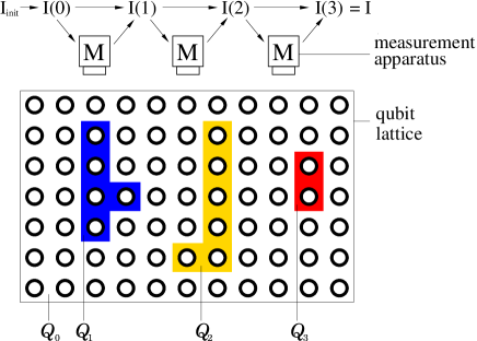
Figure 8: General scheme of the quantum computer via one-qubit measurements. The sets $Q_{t}$ of lattice qubits are measured one after the other. The results of earlier measurements determine the measurement bases of later ones. All classical information from the measurement results needed to steer the $\mbox{QC}_{\cal{C}}\;$is contained in the information flow vector ${\bf{I}}(t)$. After the last measurement round $t_{\mbox{\footnotesize{max}}}$, ${\bf{I}}(t_{\mbox{\footnotesize{max}}})$ contains the result of the computation.

Furthermore, quantum gates are not constitutive elements of the $\mbox{QC}_{\cal{C}}$; these are instead one-qubit measurements performed in a certain temporal order and in a spatial pattern of adaptive measurement bases. In fact, the most efficient temporal order of the measurements does not follow from the temporal order of the simulated gates in the network model.

The general view of a $\mbox{QC}_{\cal{C}}$-computation is as follows. The cluster ${\cal{C}}$ is divided into disjoint subsets $Q_{t}\subset{\cal{C}}$ with $0\leq t\leq t_{\mbox{\footnotesize{max}}}$, i.e. $\bigcup_{t=0}^{t_{\mbox{\tiny{max}}}}Q_{t}={\cal{C}}$ and $Q_{s}\cap Q_{t}=\emptyset$ for all $s\not=t$. The cluster qubits within each set $Q_{t}$ can be measured simultaneously and the sets are measured one after another. The set $Q_{0}$ consists of all those qubits for which no measurement bases have to be adjusted, i.e. those of which the operator $\sigma_{x}$, $\sigma_{y}$ or $\sigma_{z}$ is measured. In the subsequent measurement rounds only operators of the form $\cos\varphi\,\sigma_{x}\pm\sin\varphi\,\sigma_{y}$ are measured where $|\varphi|<\pi/2$, $\varphi\neq 0$. The measurement bases are adaptive in these rounds, i.e. they are adapted to measurement results obtained in previous rounds. The measurement outcomes from the qubits in $Q_{0}$ determine the measurement bases for the qubits in $Q_{1}$, which are measured in the second round, those from $Q_{0}$ and $Q_{1}$ together determine the bases for the measurements of the qubits in $Q_{2}$ which are measured in the third round, and so on. Finally, the result of the computation is calculated from the measurement outcomes obtained in all the measurement rounds.

Now there arises the question of how complex the required classical processing is. In principle it could be that all the obtained measurement results had to be stored separately and the functions to compute the measurement bases were so complicated that one would gain no advantage over the classical algorithm for the considered problem. This is not at all the case. If the network algorithm runs on $n$ qubits then the classical data that the $\mbox{QC}_{\cal{C}}\;$has to keep track of is entirely contained in a $2n$-component binary valued vector, which we have called the information flow vector ${\bf{I}}(t)$ QCmodel . The update of ${\bf{I}}(t)$ is a classical computation that is needed to adapt the measurement bases of cluster qubits according to previous measurement outcomes. These updates and the final identification of the computational result from ${\bf{I}}(t_{\text{max}})$ are all elementary.

Concerning the resources for the classical processing of the measurement outcomes in a $\mbox{QC}_{\cal{C}}$-computation, we point out that this processing increases the total time of computation only marginally QCmodel .

In summary, the formal description of the $\mbox{QC}_{\cal{C}}\;$is based on primitive quantities of which the most important ones are the sets $Q_{t}\subset{\cal{C}}$ of cluster qubits defining the temporal ordering of measurements on the cluster state, and the binary valued information flow vector ${\bf{I}}(t)$ which is the carrier of the algorithmic information. The reader who is interested in how this computational model arises and in its detailed description is referred to QCmodel .

III.2 Algorithms and graphs

In this section we relate $\mbox{QC}_{\cal{C}}$-algorithms to graphs. We do this by considering non-universal graph states suited for the specific algorithm in question. For the $\mbox{QC}_{\cal{C}}$, the Clifford part of each algorithm can be removed. A mathematical graph comprises all the information that needs to be kept the Clifford part.

While the network formulation of a quantum algorithm is given as a sequence of quantum gates applied to a fiducial input state, the $\mbox{QC}_{\cal{C}}$-version of a quantum algorithm is specified by a measurement pattern on the universal cluster state plus the structure QCmodel for the processing of the measurement outcomes.

The measurement pattern is, in the simplest case, just a copy of the network layout to the substrate cluster state, imprinted by the measurements. As such it contains information about the precise location of the gate simulations and about the way the “wires” connecting the gates are bent around. These are all details of the realization of an algorithm but do not belong to the description of the algorithm itself. Thus, the measurement pattern introduces a large amount of redundancy into the description of a $\mbox{QC}_{\cal{C}}$-algorithm. This redundancy may be reduced to a large extent by allowing for non-universal, algorithm-specific quantum resources.

Clearly, at this point one has to specify how special the algorithm-specific resource is allowed to be. Obviously it would make no sense to take the quantum output of the entire network as the required quantum resource and to regard the subsequent readout measurements as the algorithm. Here, we allow for any graph state Schlingel1 , (21) as the quantum resource. Graph states are both easy to create and to describe. Every algorithm may be run with a graph state as the quantum resource since the cluster state is a particular graph state.

To allow for an algorithm-specific graph state as the quantum resource of a $\mbox{QC}_{\cal{C}}$-computation reduces the redundancy of both the description and the realization of a quantum algorithm. This can easily be seen from the material presented in Section II.3. All the cluster qubits $q\in{\cal{C}}\backslash{\cal{C}}_{N}$ can be get rid of either by measuring them in the $\sigma_{z}$-eigenbasis or equivalently by not placing them initially into their positions at all. The remaining state on the sub-cluster ${\cal{C}}_{N}$ is again a cluster state. Hence it is also a graph state. It is less redundant and no longer universal.

But we can go further. Not only the qubits measured in the $\sigma_{z}$-eigenbasis may be removed from the cluster but instead all those qubits of which one of the Pauli operators $\sigma_{x}$, $\sigma_{y}$ or $\sigma_{z}$ is measured, i.e. all the qubits which form the set $Q_{0}$. The state of the unmeasured qubits that emerges after the measurement of the cluster qubits in $Q_{0}$ is again (local equivalent to) a graph state.

This may be seen as follows. First note that the operators $\sigma_{x}^{(a)}\bigotimes_{b\in V}\left(\sigma_{z}^{(b)}\right)^{\Gamma_{ab}}$ which appear in (21) form a stabilizer of the state $|\phi\{\kappa\}\rangle_{G}$. The generator of the stabilizer contains $|{\cal{C}}|$ elements for a state of $|{\cal{C}}|$ qubits. After all the qubits $q\in Q_{0}$ have been measured, the resulting state $|\Psi\rangle_{{\cal{C}}\backslash Q_{0}}$ of the $|{\cal{C}}\backslash Q_{0}|$ unmeasured qubits is again described by a stabilizer of the form

$$\begin{array}[]{r}\displaystyle{\bigotimes_{i=1}^{|{\cal{C}}\backslash Q_{0}|}\left(\sigma_{x}^{(i)}\right)^{X_{a,i}}\left(\sigma_{z}^{(i)}\right)^{Z_{a,i}}\,|\Psi\rangle_{{\cal{C}}\backslash Q_{0}}}=\displaystyle{\pm|\Psi\rangle_{{\cal{C}}\backslash Q_{0}}}\\ \displaystyle{\forall a=1\,..\,{|{\cal{C}}\backslash Q_{0}}|},\end{array}$$ (141)

with two $|{\cal{C}}\backslash Q_{0}|\times|{\cal{C}}\backslash Q_{0}|$-matrixes $X$ and $Z$, for which $X_{a,i},Z_{a,i}\in\{0,1\}$. The $|{\cal{C}}\backslash Q_{0}|\times 2|{\cal{C}}\backslash Q_{0}|$-compound matrix $(X|Z)$ is called the generator matrix of the stabilizer for $|\Psi\rangle_{{\cal{C}}\backslash Q_{0}}$. The state $|\Psi\rangle_{{\cal{C}}\backslash Q_{0}}$ is uniquely determined by the generator of its stabilizer.

The state $|\Psi\rangle_{{\cal{C}}\backslash Q_{0}}$ can thus be regarded as a $[|{\cal{C}}\backslash Q_{0}|,0,d]$-stabilizer code, with the distance $d$ not specified. Whether a code with only one code word that encodes 0 qubits should be regarded as a code in the sense of coding shall not concern us here. For the present purpose, it is important to note that the state $|\Psi\rangle_{{\cal{C}}\backslash Q_{0}}$ fulfills the assumptions of Theorem 1 in Grassl . The cited theorem states that any stabilizer code over the alphabet $A=\mathbb{F}_{p^{m}}$ is [local unitary] equivalent to a graph code. If we specialize to our case, $A=\mathbb{F}_{2^{2}}$, we find that the state $|\Psi\rangle_{{\cal{C}}\backslash Q_{0}}$ specified in (141) is local unitary equivalent to a graph state $|\phi\{\kappa\}\rangle_{G({\cal{C}}\backslash Q_{0},E_{{{\cal{C}}\backslash Q_{0}}})}$ (21).

That is, the state $|\Psi\rangle_{{\cal{C}}\backslash Q_{0}}$ needed for the computation can be obtained from a graph state $|\phi\{\kappa\}\rangle_{G({\cal{C}}\backslash Q_{0},E_{{{\cal{C}}\backslash Q_{0}}})}$ via local unitary transformations. Subsequently in the process of computation, the qubits of $|\Psi\rangle_{{\cal{C}}\backslash Q_{0}}$ are measured in their given temporal order and in the appropriate adapted bases. An alternative way to proceed is to use the graph state $|\phi\{\kappa\}\rangle_{G({\cal{C}}\backslash Q_{0},E_{{{\cal{C}}\backslash Q_{0}}})}$ directly, only modifying the measurement bases instead of performing the local rotations prior to the measurements. Thus, in a $\mbox{QC}_{\cal{C}}$-computation with a special graph state as the quantum resource and the first measurement round omitted, the way of processing the classical information is the same as in a $\mbox{QC}_{\cal{C}}$-computation with a universal resource and the first measurement round performed.

The graphs associated with states (141) are in general not unique Grassl . A constructive way to obtain graphs on ${{\cal{C}}\backslash Q_{0}}$ from $G({\cal{C}},E_{{\cal{C}}})$ and the measurement bases of the qubits in $Q_{0}$ has been described in Schlingel2 .

Now note that the measurement of the qubits in $Q_{0}$ realize the Clifford part of a quantum circuit. The fact that we can reduce the quantum resource by these qubits means that we can remove from each quantum algorithm its Clifford part. This represents, in a way, an extension to the Knill-Gottesman-Theorem GKth , stating that a quantum computation that consist only of quantum input state preparation in the computational basis, unitary gates in the Clifford group, measurement of observables in the Pauli group, and gates in the Clifford group conditioned on the outcomes of such measurements, may be simulated efficiently classically and thus requires no quantum resources at all.

With only a single non-Clifford operation in the circuit, such as a one-qubit rotation about most axes and angles, the efficient classical formalism upon which the Gottesman-Knill theorem rests can no longer be applied. The $\mbox{QC}_{\cal{C}}$-construction, on the other hand, is not affected by this. Each quantum network algorithm in question may be reduced by its Clifford part. Only the non-Clifford gates require quantum resources. The price is that the universal quantum resource, the cluster state, is changed into a non-universal, algorithm-specific resource –a graph state (21)– on fewer qubits. The Clifford part of the network algorithm specifies the corresponding graph.

In conclusion, instead of describing a quantum algorithm as a network of gates applied to some fiducial input state, a quantum algorithm may (arguably more effectively) be characterized by a graph specifying the quantum resource and the structure QCmodel for the processing of the measurement outcomes.

IV Examples of practical interest

IV.1 Multi-qubit swap gate

A multi-qubit swap gate is an $n$-qubit generalization of the two-qubit swap gate. It reverses the order of the $n$-qubits, interchanging qubit $i$ with $n+1-i$, $i=1,2,..,N$. This can be realized in a simple way on the $\mbox{QC}_{\cal{C}}\;$, as shown in Fig. 9a. The measurement pattern $\cal M$ on ${\cal{C}}_{M}$ consists of a square of $\sigma_{x}$ measurements, with sides of $2n-1$ cluster qubits. The input qubits are, simultaneously with the qubits in ${\cal{C}}_{M}$, also measured in the $\sigma_{x}$-eigenbasis.

It can be verified using the methods introduced above that realizing $\cal M$ leads to correlations between the $i$th input qubit and the $n+1-i$th output qubit. Here, we discuss the four-qubit swap as a particular example.

After the $\sigma_{x}$-measurements of the qubits in ${\cal{C}}_{M}$ we obtain for the projected state $|\psi\rangle_{{\cal{C}}(\text{swap})}$ the eigenvalue equations

$$\begin{array}[]{rcl}\displaystyle{\sigma_{x}^{(I,1)}\sigma_{x}^{(O,4)}\,|\psi\rangle_{{\cal{C}}(\text{swap})}}&=&\displaystyle{{(-1)}^{\lambda_{x,1}}|\psi\rangle_{{\cal{C}}(\text{swap})}},\\ \displaystyle{\sigma_{x}^{(I,2)}\sigma_{x}^{(O,3)}\,|\psi\rangle_{{\cal{C}}(\text{swap})}}&=&\displaystyle{{(-1)}^{\lambda_{x,2}}|\psi\rangle_{{\cal{C}}(\text{swap})}},\\ \displaystyle{\sigma_{x}^{(I,3)}\sigma_{x}^{(O,2)}\,|\psi\rangle_{{\cal{C}}(\text{swap})}}&=&\displaystyle{{(-1)}^{\lambda_{x,3}}|\psi\rangle_{{\cal{C}}(\text{swap})}},\\ \displaystyle{\sigma_{x}^{(I,4)}\sigma_{x}^{(O,1)}\,|\psi\rangle_{{\cal{C}}(\text{swap})}}&=&\displaystyle{{(-1)}^{\lambda_{x,4}}|\psi\rangle_{{\cal{C}}(\text{swap})}},\vspace{3mm}\\ \displaystyle{\sigma_{z}^{(I,1)}\sigma_{z}^{(O,4)}\,|\psi\rangle_{{\cal{C}}(\text{swap})}}&=&\displaystyle{{(-1)}^{\lambda_{z,1}}|\psi\rangle_{{\cal{C}}(\text{swap})}},\\ \displaystyle{\sigma_{z}^{(I,2)}\sigma_{z}^{(O,3)}\,|\psi\rangle_{{\cal{C}}(\text{swap})}}&=&\displaystyle{{(-1)}^{\lambda_{z,2}}|\psi\rangle_{{\cal{C}}(\text{swap})}},\\ \displaystyle{\sigma_{z}^{(I,3)}\sigma_{z}^{(O,2)}\,|\psi\rangle_{{\cal{C}}(\text{swap})}}&=&\displaystyle{{(-1)}^{\lambda_{z,3}}|\psi\rangle_{{\cal{C}}(\text{swap})}},\\ \displaystyle{\sigma_{z}^{(I,4)}\sigma_{z}^{(O,1)}\,|\psi\rangle_{{\cal{C}}(\text{swap})}}&=&\displaystyle{{(-1)}^{\lambda_{z,4}}|\psi\rangle_{{\cal{C}}(\text{swap})}}.\end{array}$$ (142)

Therein, the parameters $\lambda_{k,x},\lambda_{k,z}\in\{0,1\}$ depend linearly on the measurement outcomes $\{s_{(i,j)}\}$. Therein, $i$ is the value of the $x$- and $j$ the value of the $y$-coordinate of the respective qubit site. For example, $\lambda_{x,1}=s_{(1,2)}+s_{(2,3)}+s_{(3,4)}+s_{(4,5)}+s_{(5,6)}+s_{(6,7)}\;\text{mod}\,\,2$.

a)
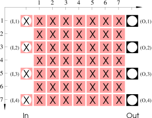
b)

Figure 9: The multi-qubit swap gate. a) measurement pattern to realize the swap gate. b) Correlation centers for two correlations of the projected state $|\psi\rangle_{{\cal{C}}(\text{swap})}$ as inherited from correlations of $|\phi\rangle_{{\cal{C}}(\text{swap})}$. The correlation $\sigma_{x}^{(I,1)}\sigma_{x}^{(O,4)}$ of $|\psi\rangle_{{\cal{C}}(\text{swap})}$ stems from the product correlation for $|\phi\rangle_{{\cal{C}}(\text{swap})}$ with the centers $a$ of basic correlation operators $K^{(a)}$ denoted by “$\circ$”. The centers of the initial correlation, which after the measurements induces the correlation $\sigma_{z}^{(I,3)}\sigma_{z}^{(O,2)}$ of $|\psi\rangle_{{\cal{C}}(\text{swap})}$, are denoted by “$\bullet$”.

The eigenvalue equations (142) can be derived from corresponding eigenvalue equations for the cluster state $|\phi\rangle_{{\cal{C}}(\text{swap})}$ on the cluster ${\cal{C}}(\text{swap})$. The required initial correlations are products of the basic correlation operators (2). The way to obtain the equations (142) is rather straightforward and therefore we omit the detailed derivations. In Fig. 9b two examples for the composition of product correlation operators from basic correlation operators $K^{(a)}$ are illustrated. The first line of (142),

$${\sigma_{x}^{(I,1)}\sigma_{x}^{(O,4)}\,|\psi\rangle_{{\cal{C}}(\text{swap})}}=\displaystyle{{(-1)}^{\lambda_{x,1}}|\psi\rangle_{{\cal{C}}(\text{swap})}},$$

for example, is derived from the eigenvalue equation

$$|\phi\rangle_{{\cal{C}}(\text{swap})}=K^{({\cal{C}}_{x,1})}|\phi\rangle_{{\cal{C}}(\text{swap})},$$ (143)

with

$$K^{({\cal{C}}_{x,1})}=\prod_{a\in{\cal{C}}_{x,1}}K^{(a)},$$ (144)

and ${\cal{C}}_{x,1}=\{(I,1),(1,2),(2,3),(3,4),(4,5),(5,6),$ $(6,7),$ $(O,4)\}$. Multiplying it out we find that all operators $\sigma_{z}$ cancel and that

$$K^{({\cal{C}}_{x,1})}=\prod_{a\in{\cal{C}}_{x,1}}\sigma_{x}^{(a)}.$$ (145)

It is now easy to see that after the $\sigma_{x}$ measurements of the qubits in ${\cal{C}}_{M}$ there remains a strict $\sigma_{x}^{(I,1)}\sigma_{x}^{(O,4)}$-correlation for the state $|\psi\rangle_{{\cal{C}}(\text{swap})}$. A similar construction can be given to obtain the $\sigma_{z}^{(I,1)}\sigma_{z}^{(O,4)}$-correlation.

With the eigenvalue equations (142) the assumptions of theorem 1 are fulfilled and thus via the described measurement pattern a unitary operation $U=SWAP$ is realized modulo a byproduct operator as specified in (84). To exchange the order of the swap-gate $U_{\text{swap}}$ and the byproduct operator $U_{\Sigma}$ the byproduct operator is conjugated under $U_{\text{swap}}$, as usual for gates in the Clifford group.

IV.2 Simulating multi-qubit Hamiltonians

Here we display a gate which simulates the unitary evolution with $U=\exp(-iH_{4}t)$ of the quantum input for the multi-particle Hamiltonian

$$H_{4}=g\,\sigma_{z}^{(1)}\sigma_{z}^{(2)}\sigma_{z}^{(3)}\sigma_{z}^{(4)}$$ (146)

and arbitrary times $t$. In addition, the gate performs a swap which can be corrected for by a subsequent swap gate as described in Section IV.1.

The procedure to realize the measurement pattern ${\cal{M}}$ for Hamiltonian simulation, as shown in Fig. 10, requires two rounds of measurements. In the first round all the $\sigma_{x}$-measurements are performed. In the second measurement round, of the qubit $(3,4)$ the operator

$$\vec{r}_{(3,4)}\cdot\vec{\sigma}=U_{z}[(-1)^{\lambda_{M}}2\varphi]\,\sigma_{x}\,U_{z}^{\dagger}[(-1)^{\lambda_{M}}2\varphi]$$ (147)

is measured, where $U_{z}[\alpha]=\exp(-i\alpha\sigma_{z}/2)$. Therein, the angle $\varphi$ is given by

$$\varphi=gt,$$ (148)

and $\lambda_{M}\in\{0,1\}$, which depends linearly on outcomes of measurements in the first round, will be specified below.

To understand the functioning of the Hamiltonian simulator let us first discuss the state $|\psi^{\prime}\rangle$ on the cluster ${\cal{C}}(\text{sim})$ after the first round of measurements. By arguments analogous to those used in Section IV.1, the state $|\psi^{\prime}\rangle$ obeys the following eigenvalue equations:

$$\begin{array}[]{rcl}\displaystyle{\sigma_{x}^{(3,4)}\sigma_{x}^{(I,1)}\sigma_{x}^{(O,4)}\,|\psi^{\prime}\rangle}&=&\displaystyle{{(-1)}^{\lambda_{x,1}}|\psi^{\prime}\rangle,}\\ \displaystyle{\sigma_{x}^{(3,4)}\sigma_{x}^{(I,2)}\sigma_{x}^{(O,3)}\,|\psi^{\prime}\rangle}&=&\displaystyle{{(-1)}^{\lambda_{x,2}}|\psi^{\prime}\rangle,}\\ \displaystyle{\sigma_{x}^{(3,4)}\sigma_{x}^{(I,3)}\sigma_{x}^{(O,2)}\,|\psi^{\prime}\rangle}&=&\displaystyle{{(-1)}^{\lambda_{x,3}}|\psi^{\prime}\rangle,}\\ \displaystyle{\sigma_{x}^{(3,4)}\sigma_{x}^{(I,4)}\sigma_{x}^{(O,1)}\,|\psi^{\prime}\rangle}&=&\displaystyle{{(-1)}^{\lambda_{x,4}}|\psi^{\prime}\rangle,\vspace{3mm}}\\ \displaystyle{\sigma_{z}^{(I,1)}\sigma_{z}^{(O,4)}\,|\psi^{\prime}\rangle}&=&\displaystyle{{(-1)}^{\lambda_{z,1}}|\psi^{\prime}\rangle},\\ \displaystyle{\sigma_{z}^{(I,2)}\sigma_{z}^{(O,3)}\,|\psi^{\prime}\rangle}&=&\displaystyle{{(-1)}^{\lambda_{z,2}}|\psi^{\prime}\rangle,}\\ \displaystyle{\sigma_{z}^{(I,3)}\sigma_{z}^{(O,2)}\,|\psi^{\prime}\rangle}&=&\displaystyle{{(-1)}^{\lambda_{z,3}}|\psi^{\prime}\rangle,}\\ \displaystyle{\sigma_{z}^{(I,4)}\sigma_{z}^{(O,1)}\,|\psi^{\prime}\rangle}&=&\displaystyle{{(-1)}^{\lambda_{z,4}}|\psi^{\prime}\rangle.}\end{array}$$ (149)

Further, the state $|\psi^{\prime}\rangle$ obeys the eigenvalue equation

$$\sigma_{z}^{(3,4)}\,\sigma_{z}^{(O,1)}\sigma_{z}^{(O,2)}\sigma_{z}^{(O,3)}\sigma_{z}^{(O,4)}\,|\psi^{\prime}\rangle={(-1)}^{\lambda}|\psi^{\prime}\rangle,$$ (150)

with $\lambda\in\{0,1\}$ linear in the measurement outcomes of the first round. Equation (150) can be easily verified with the pattern of correlation centers displayed in Fig. 10b. From (150) it follows that

$$\exp\left(i\theta\,\sigma_{z}^{(3,4)}\right)U_{4}[(-1)^{\lambda}\theta]\,|\psi^{\prime}\rangle=|\psi^{\prime}\rangle$$ (151)

for arbitrary angles $\theta$, with

$$U_{4}[\alpha]=\exp\left(-i\alpha\,\sigma_{z}^{(O,1)}\sigma_{z}^{(O,2)}\sigma_{z}^{(O,3)}\sigma_{z}^{(O,4)}\right).$$ (152)

Equation (151) is now inserted in both the l.h.s. and r.h.s. of the equations (149). For example, with the first equation from (149) one obtains

$$\begin{array}[]{rcl}\displaystyle{(-1)^{\lambda_{x,1}}\,|\psi^{\prime}\rangle}&\!=\!&\displaystyle{{\left(U_{z}[2\theta]\sigma_{x}U_{z}^{\dagger}[2\theta]\right)}^{(3,4)}\sigma_{x}^{(I,1)}\vspace{1.5mm}}\\ &&\displaystyle{\left(U_{4}[-(-1)^{\lambda}\theta]\sigma_{x}^{[4]}U_{4}^{\dagger}[-(-1)^{\lambda}\theta]\right)^{(O)}\!|\psi^{\prime}\rangle.}\end{array}$$ (153)

In the second measurement round the qubit $(3,4)$ is the only one left to be measured. As can be seen from (153), if of the operator $U_{z}[2\theta]\sigma_{x}U_{z}^{\dagger}[2\theta]$ of qubit (3,4) is measured then the state $|\psi\rangle$, into which the cluster qubits are projected after the second measurement round, obeys the eigenvalue equation

$$\begin{array}[]{l}\displaystyle{(-1)^{\lambda_{x,1}+s_{(3,4)}}\,|\psi\rangle}=\vspace{1.5mm}\\ \hskip 14.22636pt\displaystyle{\sigma_{x}^{(I,1)}\left(U_{4}[-(-1)^{\lambda}\theta]\sigma_{x}^{[4]}U_{4}^{\dagger}[-(-1)^{\lambda}\theta]\right)^{(O)}|\psi\rangle.}\end{array}$$ (154)

If we carry out this procedure for all equations in (149) we find that the state $|\psi\rangle$ that emerges after the second measurement round obeys the eigenvalue equations

$$\begin{array}[]{rcl}\displaystyle{\sigma_{x}^{(I,i)}\left(U_{4}U_{\text{swap}}\sigma_{x}^{[i]}{U_{\text{swap}}}^{\!\!\dagger}{U_{4}}^{\!\!\dagger}\right)^{(O)}|\psi\rangle}&\!\!=\!\!&\displaystyle{{(-1)}^{\lambda_{x,i}+s_{(3,4)}}\,|\psi\rangle,\vspace{1mm}}\\ \displaystyle{\sigma_{z}^{(I,i)}\left(U_{4}U_{\text{swap}}\sigma_{z}^{[i]}{U_{\text{swap}}}^{\!\!\dagger}{U_{4}}^{\!\!\dagger}\right)^{(O)}|\psi\rangle}&\!\!=\!\!&\displaystyle{{(-1)}^{\lambda_{z,i}}\,|\psi\rangle,}\end{array}$$ (155)

for $i=1\,..\,4$ and with $U_{4}$ written in short for $U_{4}[-(-1)^{\lambda}\theta]$.

With the set of equations (155) the assumptions (82) of theorem 1 are fulfilled. With theorem 1 it follows that the measurement pattern displayed in Fig. 10 realizes a unitary transformation

$$U_{\text{sim}}=U_{4}[-(-1)^{\lambda}\theta]U_{\text{swap}}U_{\Sigma},$$ (156)

where the byproduct operator is given by

$$U_{\Sigma}=\bigotimes_{i=1}^{4}\left(\sigma_{z}^{[i]}\right)^{s_{(I,i)}+\lambda_{x,i}+s_{(3,4)}}\left(\sigma_{x}^{[i]}\right)^{\lambda_{z,i}}.$$ (157)

Finally, the order of the operators has to be exchanged. Note that $U_{\text{swap}}$ and $U_{4}$ commute. From (156) one finds

$$U_{\text{sim}}=U_{\Sigma}^{\prime}U_{\text{swap}}U_{4}[-(-1)^{\lambda+\sum_{i=1}^{4}\lambda_{z,i}}\,\theta],$$ (158)

with

$$U_{\Sigma}^{\prime}=U_{\text{swap}}\,U_{\Sigma}\,{U_{\text{swap}}}^{\dagger}.$$ (159)

Thus, in order to realize $U_{4}[\varphi]$ with $\varphi$ specified in (148) we must choose

$$\theta=(-1)^{1+\lambda+\sum_{i=1}^{4}\lambda_{z,i}}\varphi.$$ (160)

That is, in the second measurement round we measure on the qubit $(3,4)$ the operator given in (147), where

$$\lambda_{M}=\left(1+\lambda+\sum_{i=1}^{4}\lambda_{z,i}\right)\;\text{mod}\,2.$$ (161)

The $\{\lambda_{x,i}\}$, $\{\lambda_{z,i}\}$ and $\lambda$ depend linearly on the measurement outcomes $\{s_{(i.j)}\}$ obtained in the first measurement round.

The sub-circuit we have described in this section simulates the unitary evolution according to a particular four-particle Hamiltonian in a two-step process of measurements. The time for which the simulated Hamiltonian acts is encoded in the basis of the measurement in the second round.

The generalization of the simulation of the 4-particle Hamiltonian $H_{4}$, shown in Fig. 10, to an arbitrary number $n$ of qubits, i.e. the simulation of the Hamiltonian $H_{n}=\bigotimes_{i=1}^{n}\sigma_{z}^{[i]}$, is straightforward.

a)
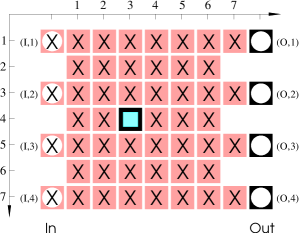
b)

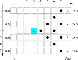
Figure 10: Simulation of the Hamiltonian $H_{4}$ as specified in eq. (146). a) measurement pattern. b) Correlation centers for additional correlation. Shaded squares (in b)) represent cluster qubits measured in adaptive bases.

IV.3 CNOT between non-neighbouring qubits

The CNOT gate described in Section II.7.7 operates on two logical qubits whose input qubits are adjacent to each other on the cluster. However, for universal quantum computation, one must be able to realize a CNOT gate between any two logical qubits. While this could be achieved using a combination of the CNOT gate, introduced above, and the swap gate, the width of the measurement pattern needed to realize this would grow linearly with the separation of the two logical qubits. There is, however, an alternative measurement pattern, which, at the cost of doubling the spacing between the input qubits on the cluster, has a fixed width.

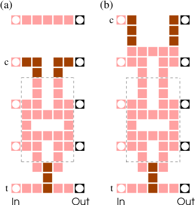
Figure 11: Measurement pattern for a CNOT gate between two logical qubits whose input and output qubits are not neighbors. Squares in light gray denote cluster qubits measured in the eigenbasis of $\sigma_{x}$, in dark gray of $\sigma_{y}$. Pattern (a) is for the case where the two qubits are separated by an odd number of logical qubits. Pattern (b) is for an even numbered separation. The patterns can be adapted to any separation by repeating the section enclosed by the dashed line. The width of the pattern remains the same for all separations.

The measurement pattern is illustrated in Fig. 11 for qubits separated by an odd and even number of logical qubits, respectively.

This layout can be understood within the quantum logic network model. The “wires” for the logical qubits in between the target- and the control qubit are crossed using the measurement sub-pattern illustrated in Fig. 12a. However, as well as swapping the qubits, this pattern also realizes the a controlled $\pi$-phase gate, also known as a controlled $\sigma_{z}$ gate, illustrated in Fig. 12b.

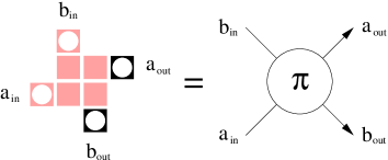
Figure 12: This measurement pattern is one of the key components of the measurement pattern in Fig. 11. It performs a conditional $\pi$-phase-gate and a swap-gate.

The quantum logic circuit realized by the whole measurement pattern, illustrated on the left-hand side of Fig. 13 uses these sub-patterns to swap the positions of adjacent qubits. This brings non-neighboring qubits together so that a CNOT operation may be performed on them.

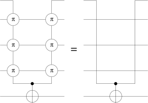
Figure 13: The measurement pattern in Fig. 11 realizes the quantum logic circuit on the left hand side of this figure. This network is equivalent to the one on the right hand side, where the only gate realized is the CNOT between the two desired non-adjacent qubits.

The networks on the left and on the right of Fig. 13 act identically, and thus the measurement pattern displayed in Fig. 11 realizes a distant CNOT-gate.

IV.4 Controlled Phase Gate

Here, we give an example of another two-qubit gate which can be realized without decomposing it into CNOTs and rotations, the controlled phase gate $U_{\text{CPG}}(\theta)$. This gate realizes the unitary operation

$$U_{\text{CPG}}[\theta]=1{\bf l}^{(ab)}+(e^{i\theta}-1)\,|11\rangle_{ab}\langle 11|,$$ (162)

applied to the two qubits $a$ and $b$.

We can write this in terms of the following one- and two-qubit rotations,

$$U_{\text{CPG}}[\theta]=e^{i\frac{\theta}{4}}U_{zz}^{(ab)}[-\theta/{2}]U_{z}^{(a)}[\theta/{2}]U_{z}^{(b)}[\theta/{2}],$$ (163)

where the two-qubit rotation is

$$U_{zz}^{(ab)}[\theta]=\exp\left(-{\rm i}\theta/2\sigma_{z}^{(a)}\sigma_{z}^{(b)}\right).$$ (164)

This representation is particularly convenient for finding the measurement pattern that realizes the gate, since rotations $U_{z}[\theta/2]$ and $U_{zz}[-\theta/2]$ are realized on the $\mbox{QC}_{\cal{C}}\;$in a simple natural way. The measurement pattern is illustrated in Fig. 14, in which the labelling of the qubits is also defined.

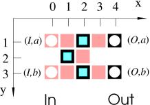
Figure 14: Controlled phase gate with additional swap.

We follow the same method as above, beginning with the eigenvalue equations of the cluster state $|\phi\rangle_{\cal C}$ on the qubits shown. The $\sigma_{x}$-measurements can be considered first, using the methods already illustrated in this paper. The resultant state of the remaining qubits $|\psi^{\prime}\rangle$, after this sub-set of the measurements has been carried out, is defined by the following set of eigenvalue equations.

$$\sigma_{x}^{(a,I)}\sigma_{x}^{(1,2)}\sigma_{x}^{(2,3)}\sigma_{x}^{(b,O)}|\psi^{\prime}\rangle =|\psi^{\prime}\rangle,$$ (165a)

$$\sigma_{x}^{(b,I)}\sigma_{x}^{(1,2)}\sigma_{x}^{(2,1)}\sigma_{x}^{(a,O)}|\psi^{\prime}\rangle =|\psi^{\prime}\rangle,$$ (165b)

$$\sigma_{z}^{(a,I)}\sigma_{z}^{(b,O)}|\psi^{\prime}\rangle =(-1)^{s_{(1,1)}+s_{(2,2)}+s_{(3,3)}}|\psi^{\prime}\rangle,$$ (165c)

$$\sigma_{z}^{(b,I)}\sigma_{z}^{(a,O)}|\psi^{\prime}\rangle =(-1)^{s_{(1,3)}+s_{(2,2)}+s_{(3,1)}}|\psi^{\prime}\rangle,$$ (165d)

and

$$\sigma_{z}^{(2,1)}\sigma_{z}^{(a,O)}|\psi^{\prime}\rangle =(-1)^{s_{(3,1)}}|\psi^{\prime}\rangle,$$ (166a)

$$\sigma_{z}^{(2,3)}\sigma_{z}^{(b,O)}|\psi^{\prime}\rangle =(-1)^{s_{(3,3)}}|\psi^{\prime}\rangle,$$ (166b)

$$\sigma_{z}^{(1,2)}\sigma_{z}^{(a,O)}\sigma_{z}^{(b,O)}|\psi^{\prime}\rangle =(-1)^{s_{(3,1)}+s_{(2,2)}+s_{(3,3)}}|\psi^{\prime}\rangle.$$ (166c)

As in section II.7.3, eigenvalue equations are now generated which commute with the remaining measurements in $\cal M$, namely the measurements of $\sigma_{xy}^{(i)}(\alpha_{i})$ on qubits $i\in\{(2,1),(1,2),(2,3)\}$. First, we manipulate the equations (166)such that, for example, the eigenvalue equation (166c) attains the form

$$\begin{array}[]{l}U_{z}^{(1,2)}[\xi]\,U_{zz}^{\left((O,a),(O,b)\right)}\left[-(-1)^{s_{(3,1)}+s_{(2,2)}+s_{(3,3)}}\xi\right]\,|\psi^{\prime}\rangle\vspace{1mm}\\ \;\;\;=|\psi^{\prime}\rangle.\end{array}$$ (167)

Similar equations containing one-qubit rotations on qubits $(2,1)$ and $(O,a)$, and $(2,3)$ and $(O,b)$ are derived from the other equations of (166) in the same way. These equations are inserted into both sides of the eigenvalue equations (165) so that, using the method introduced above, we obtain a set of four eigenvalue equations for $|\psi^{\prime}\rangle$ which induce a set of four eigenvalue equations for the state $|\psi\rangle$ that one obtains after the remaining measurements have been carried out.

Specifically, in the second measurement round the qubits $(1,2)$, $(2,1)$ and $(2,3)$ are measured. Of these qubits one measures the observables

$$\vec{r}_{a}\cdot\vec{\sigma}^{(a)}=\left(U_{z}[\alpha_{a}]\sigma_{x}U_{z}[\alpha_{a}]^{\dagger}\right)^{(a)},$$ (168)

for $a\in\{(1,2),(2,1),(2,3)\}$ and the $\{\alpha_{a}\}$ specified below.

The induced eigenvalue equations for the state $|\psi\rangle$ are of the form of equation (82), and the unitary operation realized by the gate can be read off from them using theorem 1. The full unitary operation realized by the measurement pattern is

$$\begin{array}[]{rcl}U^{\prime}U_{\Sigma}^{\prime}&=&\displaystyle{U_{zz}^{(a,b)}\bigl{[}-(-1)^{s_{(3,1)}+s_{(2,2)}+s_{{(3,3)}}}\alpha_{(1,2)}\bigr{]}U_{z}^{(a)}\bigl{[}-(-1)^{s_{(3,1)}}\alpha_{(2,1)}\bigr{]}\,U_{z}^{(b)}\bigl{[}-(-1)^{s_{{(3,3)}}}\alpha_{(2,3)}\bigr{]}U_{\text{swap}}^{(a,b)}\vspace{1mm}}\\ &&\left(\sigma_{x}^{(a)}\right)^{s_{(1,1)}+s_{(2,2)}+s_{(3,3)}}\left(\sigma_{x}^{(b)}\right)^{s_{(1,3)}+s_{{(2,2)}}+s_{(3,1)}}\left(\sigma_{z}^{(a)}\right)^{s_{(I,a)}+s_{(1,2)}+s_{(2,3)}}\left(\sigma_{z}^{(b)}\right)^{s_{(I,b)}+s_{(2,1)}+s_{(1,2)}}\end{array}$$ (169)

such that after the order of the gate and the byproduct operator is reversed, $U^{\prime}U_{\Sigma}^{\prime}=U_{\Sigma}U$, one obtains

$$\begin{array}[]{rcl}U_{\Sigma}U&=&\left(\sigma_{x}^{(a)}\right)^{s_{(1,3)}+s_{{(2,2)}}+s_{(3,1)}}\left(\sigma_{x}^{(b)}\right)^{s_{(1,1)}+s_{{(2,2)}}+s_{{(3,3)}}}\left(\sigma_{z}^{(a)}\right)^{s_{(2,1)}+s_{(1,2)}+s_{(I,b)}}\left(\sigma_{z}^{(b)}\right)^{s_{(I,a)}+s_{(1,2)}+s_{(2,3)}}\vspace{1mm}\\ &&\displaystyle{U_{zz}^{(a,b)}\bigl{[}-(-1)^{s_{(1,1)}+s_{(2,2)}+s_{(1,3)}}\alpha_{(1,2)}\bigr{]}U_{z}^{(a)}\bigl{[}-(-1)^{s_{(2,2)}+s_{(1,3)}}\alpha_{(2,1)}\bigr{]}U_{z}^{(b)}\bigl{[}-(-1)^{s_{{(1,1)}}+s_{(2,2)}}\alpha_{(2,3)}\bigr{]}U_{\text{swap}}^{(a,b)}.}\end{array}$$ (170)

Using (170) one finds the following result: To realize the controlled phase gate (162) together with a swap-gate, the observables (168) measured in the second round have to be chosen with the angles $\alpha_{(2,1)}={(-1)}^{1+s_{(2,2)}+s_{(1,3)}}\,\theta/2$, $\alpha_{(1,2)}=(-1)^{s_{(1,1)}+s_{(2,2)}+s_{(1,3)}}\theta/2$ and $\alpha_{(2,3)}=(-1)^{s_{(1,1)}+s_{(2,2)}+1}\,\theta/2$. This realizes the gate $U_{\Sigma}U_{CPG}[\theta]$, where the byproduct operator $U_{\Sigma}$ generated by the measurements may be read off from equation (170).

IV.5 Quantum Fourier transformation

To realize the quantum Fourier transform we simulate the quantum logic network given in Fig. 15a. The arrangement of the gates in this network is taken from QFT . Note that in QFT it was demonstrated that the setup to perform a quantum Fourier transformation simplifies considerably in a situation where the output state is measured right after the transformation. Here, however, the quantum Fourier transformation may constitute part of a larger quantum circuit and we do not measure its output state.

a)
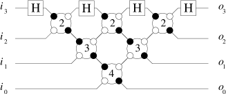
b)

Figure 15: Quantum Fourier Transformation. a) Network for quantum Fourier transformation on four qubits, taken from QFT . b) Component of the network shown in a) which performs a conditional phase- and a swap-gate. Specifically, the gate shown is $U_{CPG}[2\pi/2^{m}]$, i.e. $U_{m}=|0\rangle\langle 0|+e^{i2\pi/2^{m}}|1\rangle\langle 1|$.

As can be seen from Fig. 15, the quantum Fourier transform consists of Hadamard gates and combined gates which perform a conditional phase shift and a swap. These gates have been discussed in Sections II.2 and IV.4. All that remains to do is put the measurement patterns simulating these gates together, using the network-like composition principle described in Section II.4.

In this way we obtain a measurement pattern in which there are adjacent cluster qubits in “wires” that are measured in the $\sigma_{x}$-eigenbasis. As described in Section II.7.2, such pairs of cluster qubits may be removed from the measurement pattern. Note, that by removing adjacent pairs of $\sigma_{x}$-measured cluster qubits we have moved the $\sigma_{y}$-measurements of the Hadamard transformations “into” the subsequent conditional phase gates, i.e. we removed a cluster qubit which was not from a wire. It can be easily verified that this is an allowed extension of the method described in Section II.7.2. Finally, one obtains the $\mbox{QC}_{\cal{C}}$-circuit displayed in Fig. 16.

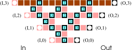
Figure 16: $\mbox{QC}_{\cal{C}}$-realization of a quantum Fourier transformation on four qubits. The cluster qubits displayed as framed squares are measured in adapted bases. For the labels see text.

In this circuit, as in all the others, the adaptive measurements are of observables

$$U_{z}[\pm\eta]\sigma_{x}U_{z}[\pm\eta]^{\dagger},$$ (171)

with $\eta=\pi/4$ for cluster qubits marked with “2” in Fig. 16, $\eta=\pi/8$ for qubits marked with “3” and $\eta=\pi/16$ for the qubits marked with “4”. The sign factors of the angles in (171) depend on the results of previous measurements.

The $\mbox{QC}_{\cal{C}}$-circuit, shown in Fig. 16 for the case of four qubits, is straightforwardly generalized to an arbitrary number $n$ of logical qubits. The temporal spatial and operational resources $T,S$ and $O$ are, to leading order

$$T=n,\;\;S,O=2n^{2}.$$ (172)

The corresponding network resources are $T_{\text{qln}}=2n$, $S_{\text{qln}}=n$ and $O_{\text{qln}}=n^{2}/2$. Thus, the scaling of the $\mbox{QC}_{\cal{C}}\;$spatial resources is worse than in the network model, but the temporal and operational resources scale in the same way as the corresponding resources for the network. The $\mbox{QC}_{\cal{C}}$-simulation of the network displayed in Fig. 15 requires half as many time steps and four times as many operations, albeit only one-qubit operations.

IV.6 Multi-qubit controlled gates

In this section we describe the realization of the Toffoli phase gate and the three-qubit controlled gate $CARRY$ which we will both need for the construction of the $\mbox{QC}_{\cal{C}}$-adder circuit described in Section IV.7.

The Toffoli phase gate is a three-qubit generalization of the two-qubit controlled phase gate. If all three qubits are in the state $|1\rangle$, the state gains a phase of $\exp({\rm i}\phi)$, while all other logical basis states remain unchanged by the gate,

$$U_{\text{Toffoli}}^{(c_{1},c_{2},t)}[\phi]=1{\bf l}^{(c_{1},c_{2},t)}+(e^{i\phi}-1)\,|111\rangle_{c_{1},c_{2},t}\langle 111|.$$ (173)

Like the controlled phase gate it can be represented as a product of multi-qubit rotations,

$$\begin{split}U_{\text{Toffoli}}^{(c_{1},c_{2},t)}[\phi]=\,&U_{zzz}^{(c_{1},c_{2},t)}\!\left[\frac{\phi}{4}\right]U_{zz}^{(c_{1},c_{2})}\!\left[-\frac{\phi}{4}\right]U_{zz}^{(c_{1},t)}\!\left[-\frac{\phi}{4}\right]\\ &U_{zz}^{(c_{2},t)}\!\left[-\frac{\phi}{4}\right]U_{z}^{(c_{1})}\!\left[\frac{\phi}{4}\right]U_{z}^{(c_{2})}\!\left[\frac{\phi}{4}\right]U_{z}^{(t)}\!\left[\frac{\phi}{4}\right].\end{split}$$ (174)

where we have dropped the global phase, and $U_{zzz}^{(c_{1},c_{2},t)}[\alpha]=\exp\left(-{\rm i}\alpha/2\sigma_{z}^{(c_{1})}\sigma_{z}^{(c_{2})}\sigma_{z}^{(t)}\right)$ is a three qubit generalized rotation. The two-qubit rotations $U_{zz}$ are as defined in (164).

The way to convert the sequence (174) of generalized rotations into a measurement pattern is as in the examples before. The measurement layout for the Toffoli phase gate is illustrated in Fig. 17. Each of the generalized rotations that make up the gate is directly associated with of one of the measurements made in the eigenbasis of $U_{z}[\pm\phi/4]\sigma_{x}U_{z}[\pm\phi/4]^{\dagger}$. An initial cluster-state correlations which is used for the realization of a generalized rotation is shown in Fig. 18: the rotation $U_{zz}^{(c_{1},c_{2})}[\phi/4]$ is realized via the measurement of the cluster qubit at the lattice site $(3,1)$ in the appropriate basis.

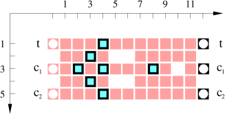
Figure 17: A measurement layout to realize a Toffoli phase gate with phase $\phi$. The qubits marked by black boxes are simultaneously measured in adapted bases depending on previous measurement outcomes.

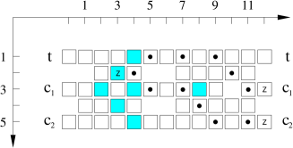
Figure 18: Cluster state quantum correlations for the realization of $U_{zz}^{(c_{1},c_{2})}[\phi/4]$, used in the Toffoli phase gate.

The sign factors of the angles that specify the measurement bases depend on the outcome of $\sigma_{x}$-measurements only. Thus, after all $\sigma_{x}$- measurements have been performed, the measurement bases for the remaining qubits can be deduced and the Toffoli phase-gate is realized in a single further time-step. The measurement pattern realizes the generalized rotations directly and is not derived from a quantum logic network.

Now we describe the realization of a four-qubit gate $CARRY$, which has one target and three control qubits. It performs a phase-flip $\sigma_{z}$ on the target if at least two of the control qubits are in state $|1\rangle$ and otherwise does nothing, i.e.

$$U_{CARRY}=\exp\left(-i\pi\!\!\!\!\sum_{i=000_{d}\,|\,w(i)\geq 2}^{111_{d}}\!\!\!\!\!|i\rangle_{c_{1}c_{2}c_{3}}\langle i|\otimes|1\rangle_{t}\langle 1|\right),$$ (175)

Expanding the projectors on the control qubits into products of Pauli operators one obtains

$$\begin{array}[]{rcl}U_{CARRY}&=&\displaystyle{e^{-i\frac{\pi}{4}}\underbrace{\exp\left(-i\frac{\pi}{8}\sigma_{z}^{(t)}\sigma_{z}^{(c_{3})}\right)}_{U_{i}}\underbrace{\exp\left(-i\frac{\pi}{8}\sigma_{z}^{(t)}\sigma_{z}^{(c_{2})}\right)}_{U_{h}}\underbrace{\exp\left(i\frac{\pi}{8}\sigma_{z}^{(c_{3})}\right)}_{U_{g}}\underbrace{\exp\left(i\frac{\pi}{8}\sigma_{z}^{(c_{2})}\right)}_{U_{f}}\underbrace{\exp\left(i\frac{\pi}{8}\sigma_{z}^{(c_{1})}\right)}_{U_{e}}}\\ &&\displaystyle{\underbrace{\exp\left(i\frac{\pi}{4}\sigma_{z}^{(t)}\right)}_{U_{d}}\underbrace{\exp\left(-i\frac{\pi}{8}\sigma_{z}^{(t)}\sigma_{z}^{(c_{1})}\right)}_{U_{c}}\underbrace{\exp\left(-i\frac{\pi}{8}\sigma_{z}^{(c_{1})}\sigma_{z}^{(c_{2})}\sigma_{z}^{(c_{3})}\right)}_{U_{b}}\underbrace{\exp\left(i\frac{\pi}{8}\sigma_{z}^{(t)}\sigma_{z}^{(c_{1})}\sigma_{z}^{(c_{2})}\sigma_{z}^{(c_{3})}\right)}_{U_{a}}.}\end{array}$$ (176)

The global phase is henceforth discarded.

The unitary transformation is now subdivided into two parts,

$$U_{CARRY}=U_{h,i}\,U_{a-g},$$ (177)

with $U_{a-g}=U_{g}U_{f}U_{e}U_{d}U_{c}U_{b}U_{a}$ and $U_{h,i}=U_{i}U_{h}$. Correspondingly, the cluster on which $U_{CARRY}$ is realized is divided into two sub-clusters. On the first sub-cluster the transformations $U_{a}$ to $U_{g}$ are realized, on the second sub-cluster $U_{h,i}$. The measurement pattern to realize $U_{CARRY}$ is displayed in Fig. 19. The first sub-cluster stretches from $x=0$ to $x=8$, with the input at $x=0$ and the intermediate output at $x=8$. The qubits with $8\leq x\leq 16$ belong to the second sub-cluster.

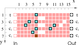
Figure 19: The three qubit controlled gate. Qubits displayed as squares in light gray are measured in the $\sigma_{x}$-eigenbasis, the qubit displayed in dark gray is measured in the $\sigma_{y}$-eigenbasis, and the measurement bases of the qubits displayed as framed squares are adaptive.

Let us now explain the sub-gate $U_{a-g}$. The conversion of the sequence (176) of generalized rotations is as in the previous examples. For each generalized rotation there is one cluster qubit in ${\cal{C}}_{M}(U_{a-g})$ whose measurement basis specifies the respective rotation angle. Specifically, the measurement of the cluster qubit $(3,4)$ sets the rotation angle of $U_{a}$, the measurement of qubit $(4,3)$ sets the angle for $U_{b}$, $(5,6)$ sets $U_{c}$, $(6,7)$ sets $U_{d}$, $(6,5)$ sets $U_{e}$, $(6,3)$ sets $U_{f}$ and qubit $(6,1)$ sets $U_{g}$. The quantum correlations of the initial cluster state which induce via the measurements of the cluster qubits in ${\cal{C}}_{M}(U_{a-g})$ the quantum correlations associated with the generalized rotations are displayed in Fig. 20.

The realization of the gate requires two measurement rounds. In the first round the standard measurements of $\sigma_{x}$ and $\sigma_{y}$ are performed. Note that the rotation angle of $U_{d}$ is twice as big as for the other rotations. To realize $U_{d}$ of the cluster qubit $(6,7)$ the observable

$$U_{z}\left[\pm\frac{\pi}{4}\right]\,\sigma_{x}U_{z}\left[\mp\frac{\pi}{4}\right]=\pm\sigma_{y}$$ (178)

is measured. Thus, the realization of $U_{d}$ belongs to the first round of measurements. Strictly speaking, this measurement round does not belong to the gate but to the circuit as a whole since all standard measurements are performed simultaneously.

a)	b)
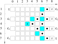
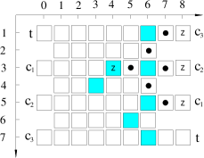
c)	d)

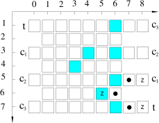
Figure 20: Quantum correlations of the initial cluster state $|\phi\rangle_{{\cal{C}}(U_{a-g})}$ on the cluster ${\cal{C}}(U_{a-g})$. These correlations induce via the $\sigma_{x}$-measurements the quantum correlations for the state $|\psi^{\prime}\rangle$ which act only on the output qubits and one cluster qubit in ${\cal{C}}_{M}(U_{a-g})$. The pattern of correlation centers in a) displays the correlation required to realize $U_{a}$; b),c) and d) display the correlations for $U_{b}$, $U_{c}$ and $U_{e}$, respectively. The correlations used for the realization of $U_{d}$, $U_{f}$ and $U_{g}$ are not shown. They are analogous to the one in d) used for the realization of $U_{e}$.

In the second measurement round, of the remaining qubits in ${\cal{C}}_{M}(U_{a-g})$ one measures the observables

$$U_{z}\left[\pm\frac{\pi}{8}\right]\,\sigma_{x}U_{z}\left[\mp\frac{\pi}{8}\right].$$ (179)

The procedure to infer the sign factors in (179) and (178) is explained in Section II.6.

The reason why the measurements in the tilted bases may all be performed simultaneously in the second round can be seen as follows. Be $Q_{\nearrow}$ the set of qubits measured in tilted bases. The contribution $U_{\Sigma,Q_{\nearrow}}$ of the cluster qubits measured in tilted bases to the byproduct operator $U_{\Sigma}$ in (84) contains only a $z$-part but no $x$-part. That is, it has the form

$$U_{\Sigma,Q_{\nearrow}}=\bigotimes_{i\in I\subset\{t,c_{1},c_{2},c_{3}\}}\sigma_{z}^{[i]}.$$ (180)

In (83) the byproduct operator appears “on the wrong side” of $U_{a-g}$ as does the contribution $U_{\Sigma,Q_{\nearrow}}$. When the order of the gate and the byproduct operator is exchanged, the byproduct operator may modify the gate. While this is, not surprisingly, indeed the case for the whole $U_{\Sigma}$, it is not so for the contribution $U_{\Sigma,Q_{\nearrow}}$ coming from the measurements in the tilted bases. Because $U_{\Sigma,Q_{\nearrow}}$ has only a $z$-part it commutes with $U_{a-g}$. Therefore, the results of measurements in a tilted basis do not mutually affect the choice of their measurement bases.

The fact that hat the byproduct operator $U_{\Sigma,Q_{\nearrow}}$ is indeed of form (180) we do not show here explicitly. For the byproduct operator created in the measurement of qubit $(3,4)$ realizing the transformation $U_{a}$ it may be verified from equation (157) in Section IV.2.

The explanation of the second sub-gate, $U_{h,i}$, is analogous. Fig. 21 displays the quantum correlations of the initial cluster state which, via the measurements in ${\cal{C}}_{M}(U_{h,i})$, induce the required quantum correlations associated with $U_{h}$ and $U_{i}$.

a)	b)

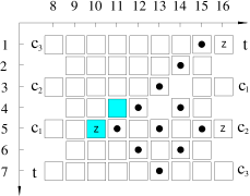
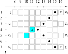
Figure 21: Quantum correlations of the initial cluster states on ${\cal{C}}(U_{h})$ and ${\cal{C}}(U_{i})$. These correlations induce, via the $\sigma_{x}$-measurements, the quantum correlations for the states $|\psi^{\prime}\rangle_{{\cal{C}}(U_{h})}$ and $|\psi^{\prime}\rangle_{{\cal{C}}(U_{i})}$ that involve only the respective output qubits and one qubit in the gate body. The pattern of correlation centers in a) displays the correlation required to realize $U_{h}$ and b) the correlation for $U_{i}$.

Two further points we would like to address in this section. The first is to note that the whole gate $U_{CARRY}$ can be performed on the $\mbox{QC}_{\cal{C}}\;$in two measurement rounds. The first measurement round is that of the $\sigma_{x}$-, $\sigma_{y}$- and $\sigma_{z}$-measurements which, strictly speaking, does not belong to the gate but to the circuit as a whole. The second measurement round is that of the simultaneous measurements in tilted measurement bases.

We have already seen that the measurements that realize the unitary transformations $U_{a},\,..\,,U_{g}$ may be realized simultaneously, and this argument may be extended to the entire gate $U_{CARRY}$. All the byproduct operators created with the measurements in tilted bases have only a $z$- but no $x$-part. Therefore they all commute with $U_{CARRY}$. Thus, to choose the right measurement bases neither of the measurements in a tilted basis that realizes one of the rotations $U_{a},\,..\,,U_{i}$ needs to wait for another measurement in a tilted basis.

Second, note that the for $U_{CARRY}$ the target-input and the target-output can be interchanged, see Fig. 22. This holds because the (conditional) phase-flip on the target qubit is its own inverse. Thus, the target qubit may travel through the gate backwards. This property also holds for the Toffoli phase gate. We will make use of it in the construction of the quantum adder in the next section.

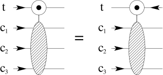
Figure 22: In the three-qubit controlled gate $CARRY$, the target qubit may travel either back or forth.

IV.7 Circuit for addition

The $\mbox{QC}_{\cal{C}}$-version of the quantum adder corresponds to the quantum logic network as given in AdderNW , see Fig. 23. In this paper we use the three-qubit controlled phase gate $CARRY$ together with a prior and subsequent Hadamard gate on the target qubit while in AdderNW the equivalent three-qubit controlled spin-flip gate is used directly.

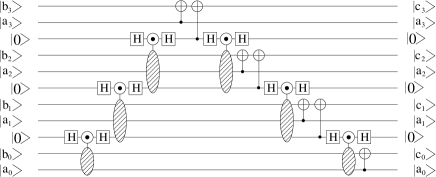
Figure 23: Quantum logic network for 4-qubit adder, $c=a+b\;\text{mod}\,2^{4}$. The adder network is taken from AdderNW . The two-qubit controlled gate in this network is the Tofolli phase gate as discussed in Section IV.6. A straightforward simulation of this network on the $\mbox{QC}_{\cal{C}}\;$would result in a quadratic scaling of spatial resources. However, the more compact realization discussed below requires only a linear overhead.

At first sight it appears as if the horizontal dimension of the cluster to realize the adder circuit would grow linearly with the number of logical qubits $n$. This is, however, not the case. The $\mbox{QC}_{\cal{C}}$-circuit may be formed in such a way that the horizontal size of the required cluster is constant such that the cluster size increases only linearly with the number $n$ of logical qubits. To see what the $\mbox{QC}_{\cal{C}}$-realization of the quantum adder will look like, the network displayed in Fig. 23 may be bent in a way displayed in Fig. 24.

To “bend a network” is a rather informal notion. We therefore now specify what we mean by this. If a quantum circuit is displayed as a quantum logic network, the vertical axis usually denotes some spatial dimension, i.e. the location of the qubit carriers, and the horizontal axis corresponds to the sequence of steps of a quantum computation, i.e. a logical time. As the basic blocks of quantum computation in the network model, the universal gates, are unitary transformations generated by suitably chosen Hamiltonians the logical time becomes associated with physical time. This is, however, a peculiarity of the network model. If on the $\mbox{QC}_{\cal{C}}\;$a quantum logic network is simulated, the temporal axis is converted into an additional spatial axis. The temporal axis in a $\mbox{QC}_{\cal{C}}$-computation emerges anew. It has no counterpart in the network model. If we modify a quantum logic network in such a way that qubits travel from right to left, as done in Fig. 24, it does not mean that we propose to use particles that travel backwards in time because we do not need to respect the temporal axis implied by the network model. If one wants a semi-network picture that accounts for this, one may imagine the logical qubits as traveling through pipes on a two-dimensional surface.

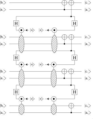
Figure 24: Quantum logic network for 4-qubit adder, bent.

The reason why we may let the auxiliary qubits travel “backwards” is the identity displayed in Fig. 22. This arrangement of gates makes the circuit more compact. To complete the description of components from which the $\mbox{QC}_{\cal{C}}$-version of the quantum adder is built, a compact measurement pattern for the two combined CNOT-gates is displayed in Fig. 25.

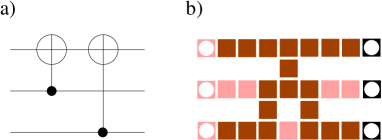
Figure 25: Combination of two CNOT-gates (a) and its $\mbox{QC}_{\cal{C}}$-realization (b).

The realization of the quantum adder in the network layout of Fig. 24 directly leads to the $\mbox{QC}_{\cal{C}}$-circuit for the quantum adder displayed in Fig. 26. Please note that the displayed $\mbox{QC}_{\cal{C}}$-adder is for eight qubits while the networks in Figs. 23 and 24 are only for four qubits.

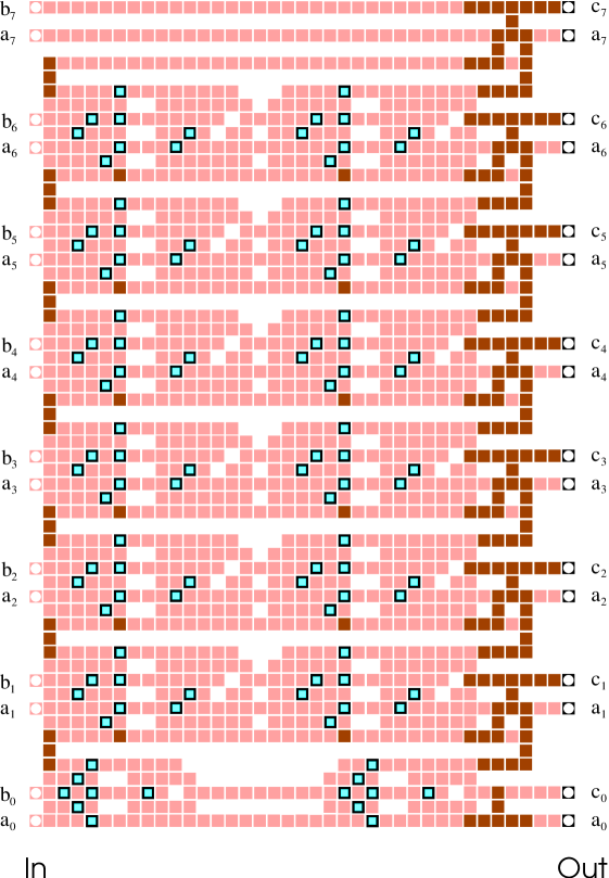
Figure 26: Quantum adding circuit for two 8-qubit states. As in all figures displaying $\mbox{QC}_{\cal{C}}$-circuits, squares in light and dark gray represent cluster qubits measured in the $\sigma_{x}$- and $\sigma_{y}$-eigenbasis, respectively. The measurement bases of qubits displayed as framed squares are adaptive.

For the quantum adder circuit in Fig. 26 we have made two further minor simplifications. The first concerns the ancilla preparation. To prepare an ancilla qubit on the cluster in the state $|+\rangle$ means to measure the respective cluster qubit in the $\sigma_{x}$-eigenbasis (the randomness of the measurement outcome does not jeopardize the deterministic character of the circuit). As can be seen from the Toffoli gate and the three-qubit controlled gate displayed in Figs. 17 and 19, the ancilla qubits are located on cluster qubits which have only one next neighbor. As can be verified from the eigenvalue equations (1), to measure a qubit of a cluster state which only has one next neighbor in the eigenbasis of $\sigma_{x}$ also has the effect of projecting this neighboring cluster qubit into an eigenstate of $\sigma_{z}$. Such cluster qubits may be removed from the cluster as explained in Section II.3. With these neighboring qubits removed the cluster qubits on which the initial ancilla qubits were located become disconnected from the remaining cluster and may thus be removed as well. With the same argument, the cluster qubits carrying the ancillas in their output state, and their next neighbors may also be removed.

Second, between the $\mbox{QC}_{\cal{C}}$-realization of the CARRY-gates on the left and the subsequent blocks of CNOT-gates we have removed pairs of adjacent cluster qubits that would be measured in the eigenbasis of $\sigma_{x}$. Why this can be done has been explained for adjacent qubits in wires in Section II.7.2. Here the situation is a little more involved since, like in case of the circuit for Fourier transformation displayed in Section IV.5, one of the removed qubits in each pair has more than two neighbors. But the method still works as can be easily verified.

Let us now briefly discuss the resources required for the $\mbox{QC}_{\cal{C}}$-realization of an $n$-qubit adder. As can be seen directly from the circuit displayed in Fig. 26 and the underlying network shown in Fig. 24 with its repeating sub-structure, the adder requires a cluster of height $8n-5$ and of constant width $38$. Thus the spatial and operational resources are, to leading order,

$$S=O=304\,n.$$ (181)

Concerning the temporal resources note that each pair of three-qubit controlled phase gates using the same control qubits and the pair of Toffoli phase gates may be completed at one time instant but that one pair of gates is completed after another. The reason why the measurements in the tilted bases that complete each pair of gates may be performed simultaneously is the same as the one given previously for the measurements in tilted bases of a single three-qubit controlled gate. The propagation of byproduct operators is most easily followed in the network of Fig. 23. The temporal complexity $T$ of an $n$-qubit $\mbox{QC}_{\cal{C}}$-adder is

$$T=n,$$ (182)

plus one step of $\sigma_{x}$-,$\sigma_{y}$- and $\sigma_{z}$-measurements for the entire circuit.

The corresponding network resources are to leading order $S_{\text{qln}}=3n$ and $O_{\text{qln}}=T_{\text{qln}}=8n$. For the counting of the operational and temporal network resources we have assumed that the three-qubit controlled spin-flip gate used in the addition circuit is composed of two Toffoli gates and one CNOT-gate as described in AdderNW , and that the CNOT- and the Toffoli-gate are regarded as elementary.

Thus we find for both the network and the $\mbox{QC}_{\cal{C}}$-realization of the quantum adder that the spatial, temporal and operational resources scale linearly with $n$. Therefore, the resource overheads in one realization as compared to the other one are only constant. For the $\mbox{QC}_{\cal{C}}\;$this is much better than what is indicated by the bounds (138), (139) and (140), in particular for the spatial and operational resources. Equation (139) yields an upper bound on $S$ which is $\sim n^{3}$ and (140) gives bounds on $O$ and $S$ which are $\sim n^{2}$. Thus, the quantum adder is an example for which these bounds are very loose. In general they should not be mistaken as estimates.

If the pre-factors are compared, one finds that for the realization of a quantum adder the $\mbox{QC}_{\cal{C}}\;$requires about 100 times more spatial and 38 times more operational resources, while it is 8 times faster. However, since we compare different objects these ratios do not mean much apart from the fact that they are constant. It may be argued that in case of the $\mbox{QC}_{\cal{C}}\;$spatial resources are not as precious as they usually are, for to create cluster states one needs a system with non-selective uniform interaction only while for quantum logic networks one generally requires a system with selective interactions among the qubits. Concerning the operational and temporal resources, the $\mbox{QC}_{\cal{C}}\;$only uses one-qubit measurements while the corresponding network uses two- and three-qubit gates as elementary operations.

IV.8 Remarks

We would like to add two remarks, one with regard to the elementary constituents of the $\mbox{QC}_{\cal{C}}$, and one with regard to their composition principle.

For the particular set of gate simulations used in the $\mbox{QC}_{\cal{C}}\;$universality proof in Section II, the CNOT-gate and arbitrary one-qubit rotations, there is only a single instance of where one of these gates has been used as part of a more complicated gate in all examples of this section. Namely, the next-neighbor CNOT-gate has been used as part of the long-distance CNOT described in Section IV.3. Of universal gate simulations one might expect that any circuit is composed of them rather that they occur almost not at all. One could say, though, that the used set of gates is not a good choice for the universal set. In fact, in realizations of network quantum computers it is often the physics of the specific implementation that determines which gates are elementary. For the $\mbox{QC}_{\cal{C}}\;$this is not so. The $\mbox{QC}_{\cal{C}}\;$may simulate, for example, general one-qubit rotations and Toffoli gates alike. Any gate simulation may be called “elementary” with the same right as any other, but they cannot be all elementary. The elementary constituents of the $\mbox{QC}_{\cal{C}}\;$are not gate simulations.

As a consequence, the composition principle for these elements will be different from gate composition. At first sight, if we go through the examples of this section, we find that this is not yet reflected in the larger and more complicated constructions. For the quantum Fourier transform and the addition circuit we have, though playing with some tricks, ultimately imitated network composition.

However, in the smaller gates and sub-circuits such as the controlled phase gate, the Toffoli phase gate and the gate $CARRY$ we find something that might give rise to a new and more appropriate composition principle. First, for the $\mbox{QC}_{\cal{C}}\;$it is not the one-qubit and two-qubit operations that are particularly simple. In the Hamiltonian simulation circuit of Section IV.2 we found that it is easy to realize generalized rotations $\exp(i\varphi\,\sigma^{(J)})$ where $\sigma^{(J)}$ is a composite Pauli operator, $\sigma^{(J)}=\bigotimes_{a\in J}\sigma_{k_{a}}^{(a)}$, $k_{a}=x,y,z$. Furthermore, in the subsequent examples of the multi-qubit gates in Sections IV.4 and IV.6 we have decomposed the gates into such generalized rotations rather than into known standard gates on fewer qubits.

Any unitary transformation may be decomposed into a unitary transformation in the Clifford group followed by generalized rotations. So, is this a new composition principle? With our present state of knowledge, the answer must be “Not yet.”. First, though any transformation may be rewritten in this form, it is presently not clear how to design quantum algorithms with these elements directly. Second, the construction uses the very concept of applying unitary transformations to the state of a quantum register. However, as we have explained in QCmodel and also briefly sketched in Section III.1, the $\mbox{QC}_{\cal{C}}\;$has no quantum register. So, the generalized rotations and their concatenation at least have to be reformulated to fit the description of the $\mbox{QC}_{\cal{C}}$. In particular, they have to be made compatible with the graph states identified in Section III.2 as characteristic quantum resource to represent algorithms. Nevertheless, it appears that the generalized rotations should be reflected in what may emerge as elementary constituents and composition principle for the $\mbox{QC}_{\cal{C}}$.

V Computation with limited spatial resources and in the presence of decoherence

In this section we describe how to perform $\mbox{QC}_{\cal{C}}$-computation on finite and possibly small clusters. If the cluster that may be provided by a specific device is too small for a certain measurement pattern it does not mean that the respective $\mbox{QC}_{\cal{C}}$-algorithm cannot be run on this device. Instead, the $\mbox{QC}_{\cal{C}}$-computation may be split into several parts such that each of those parts fits on the cluster.

To see this consider Scheme 1 for the realization of gates. Scheme 1 is applicable to any gate or sub-circuit. It is thus possible to divide the circuit into sub-circuits each of which fits onto the cluster. The adapted scheme is a process of repetitive re-entangling steps alternating with rounds of measurements.

Specifically, one starts with the realization of the first sub-circuit acting on the fiducial input state located on $I_{1}\subset{\cal{C}}$. The fiducial input is, while being processed, teleported to some subset $O_{1}$ of the cluster ${\cal{C}}$. The set $O_{1}$ of qubits forms the intermediate output of the first sub-circuit. These qubits remain unmeasured while all the other qubits are measured to realize the first sub-circuit. Now the realization of the second sub-circuit begins. Its input state has already been prepared, $I_{2}=O_{1}$. The cluster qubits $a\in{\cal{C}}\backslash O_{1}$ which have been measured in the realization of the first sub-circuit are now prepared individually in the state $|+\rangle_{a}$. This completes step 1 of Scheme 1 to realize the second sub-circuit. Step 2 is to entangle the whole cluster via the Ising interaction. In the third step all cluster qubits except those of the intermediate output $O_{2}$ are measured whereby the realization of the second sub-circuit is completed. The intermediate output is now located on $O_{2}$. For the realization of the subsequent sub-circuits one proceeds accordingly.

An advantage of this modified procedure is that one gets by with smaller clusters. A disadvantage is that the Clifford part of the circuit may no longer be performed in a single time step.

Perhaps the most important advantage of the above construction is that in this way a basic requirement to make the $\mbox{QC}_{\cal{C}}\;$fault-tolerant can be fulfilled. Namely, decoherence can be controlled. If a single large cluster is used the computation might reach certain cluster qubits only after a long time such that the cluster would have already decohered significantly and it is not clear how error-correction could help in such a situation. This might, for any error rate, limit the duration of a computation. On the contrary, if the computation is split then the size of the sub-circuits may be adjusted such that each of them can be performed within a fixed time $T$ and in this way, each cluster qubit is, before being measured, exposed to a bounded amount of decoherence specified by $T$. Thus, “fresh” qubits for computation are always provided.

VI Conclusion

In this paper we have given a detailed account of the one-way quantum computer. We have shown that the $\mbox{QC}_{\cal{C}}\;$can be regarded as a simulator of quantum logic networks. This way, we clarified the relation of the $\mbox{QC}_{\cal{C}}\;$to the network model of quantum computation and gave the universality proof.

We have based our description on the correlations exhibited by cluster states, and states that can be created from them under one-qubit measurements. For this purpose, theorem 1 of Section II.6 is an important tool. It relates unitary transformations to quantum correlations exhibited by certain pure states.

In Section IV we have presented a number of example circuits such as the circuit for quantum Fourier transformation and for addition. In this way, hopefully, we also have acquainted the reader with a number of construction principles for $\mbox{QC}_{\cal{C}}$-circuits. Note that the simulations of the universal gates required in the universality proof are hardly used. Instead, more compact measurement patterns have been found.

The main purpose of this paper has been to provide a comprehensive description of the $\mbox{QC}_{\cal{C}}\;$from the network perspective. Beyond that, we have pointed out the non-network aspects of the $\mbox{QC}_{\cal{C}}$, such as the different nature of information processing QCmodel ; QCmodelsum , and the connection to mathematical graphs.

Appendix A Cluster decomposition

In Section II.1 we have associated the cluster state ${|\phi_{\{\kappa\}}\rangle}_{{\cal{C}}_{N}}$ on a cluster ${\cal{C}}_{N}$ with a graph $G({\cal{C}}_{N},E_{{\cal{C}}_{N}})$ where the set $E_{{\cal{C}}_{N}}$ of edges is defined in the same way as in (22) for $E_{\cal{C}}$. To decompose the cluster means in more precise terms to decompose the associated graph $G({\cal{C}}_{N},E_{{\cal{C}}_{N}})$ into subgraphs, that is we decompose both the set of vertices, ${\cal{C}}_{N}$, and the set of edges, $E_{{\cal{C}}_{N}}$. As in (48), the set of vertices is decomposed into the subsets ${\cal{C}}(g_{i})$, the sub-clusters corresponding to the gates $g_{i}$,

$${\cal{C}}_{N}=\bigcup_{i=1}^{|{\cal{N}}|}{\cal{C}}(g_{i}).$$

Herein, the sets ${\cal{C}}(g_{i})$ are overlapping. The output vertices of some sub-cluster ${\cal{C}}(g_{k})$, corresponding to the output cluster qubits of the gate $g_{k}$, form –if they are not the output vertices of the whole graph– (some of) the input vertices of other sub-clusters $\big{\{}{\cal{C}}(g_{l})\big{\}}$. We define the sets $I$ and $O$ of input and output vertices of ${\cal{C}}_{N}$, and the set of overlapping vertices $V_{I/O}$ as follows:

$$\begin{array}[]{rcl}I&=&\displaystyle{\big{\{}a\in{\cal{C}}_{N}:\,\exists i\,|\,a\in{\cal{C}}_{I}(g_{i})\,\wedge\,\neg\exists j\,|\,a\in{\cal{C}}_{O}(g_{j})\big{\}}\vspace{2mm}}\\ O&=&\displaystyle{\big{\{}a\in{\cal{C}}_{N}:\,\neg\exists i\,|\,a\in{\cal{C}}_{I}(g_{i})\,\wedge\,\exists j\,|\,a\in{\cal{C}}_{O}(g_{j})\big{\}}\vspace{2mm}}\\ V_{I/O}&=&\big{\{}a\in{\cal{C}}_{N}:\,\exists i\,|\,a\in{\cal{C}}_{I}(g_{i})\,\wedge\,\exists j\,|\,a\in{\cal{C}}_{O}(g_{j})\big{\}}.\vspace{2mm}\end{array}$$ (183)

In the same way as we decompose the set of vertices, ${\cal{C}}_{N}$, into subsets ${\cal{C}}(g_{i})$, according to (49), we decompose the set of edges, $E_{{\cal{C}}_{N}}$, into subsets $E(g_{i})$,

$$E_{{\cal{C}}_{N}}=\bigcup_{i=1}^{|{\cal{N}}|}E(g_{i}).$$

Now, for the decomposition to be useful, the subsets ${\cal{C}}(g_{i})$ and $E(g_{i})$ must fulfill a number of constraints. The first of them is that each pair $({\cal{C}}(g_{i}),E(g_{i}))$ is again a graph, $G({\cal{C}}(g_{i}),E(g_{i}))$. As in (51), this requires in particular, that the endpoints of all the edges in $E(g_{i})$ are in ${\cal{C}}(g_{i})$,

$$\forall\,a\in{\cal{C}}_{N}\,|\,(\exists e\in E(g_{i})\,\,\text{s.th.}\,a\in e):\,\,a\in{\cal{C}}(g_{i}).$$

This already excludes a cluster ${\cal{C}}_{N}$ as displayed in Fig. 27a. There, the cluster ${\cal{C}}_{N}$ is decomposed into sub-clusters ${\cal{C}}(g_{1})$ and ${\cal{C}}(g_{2})$. But there are edges, namely those which connect ${\cal{C}}(g_{2})$ and ${\cal{C}}(g_{1})$, which can neither be included in $G({\cal{C}}(g_{1}),E(g_{1}))$ nor $G({\cal{C}}(g_{2}),E(g_{2}))$. Therefore, condition (49) cannot be satisfied and consequently the decomposition of ${\cal{C}}_{N}$ into ${\cal{C}}(g_{1})$ and ${\cal{C}}(g_{2})$ is not allowed.

It is necessary to exclude a decomposition as in Fig 27a as the circuit displayed there cannot be understood from its components on the sub-clusters ${\cal{C}}(g_{1})$ and ${\cal{C}}(g_{2})$. The reason for this is that the cluster states on the sub-clusters ${\cal{C}}(g_{1})$ and ${\cal{C}}(g_{2})$ are mutually entangled. This is caused by precisely those interactions $S^{ab}$ that correspond to the edges in $E_{{\cal{C}}_{N}}$ which could not be included in either of the subgraphs.

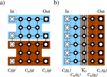
Figure 27: Two forbidden divisions of a cluster into sub-clusters. The functioning of the 4-qubit gate in a) cannot be understood from the functioning of the two 2-qubit gates on the sub-clusters. The displayed subdivision is excluded by constraint (51). The situation in b) can be treated with a careful assignment of the edges to the subgraphs. In this paper, however, it is excluded for simplicity by the assignment (184) together with the constraint (185).

The central condition (50) is that, in contrast to the sets of vertices ${\cal{C}}(g_{i})$, the sets of edges $E(g_{i})$ do not overlap,

$$\forall i,j=1\,..\,|{\cal{N}}|,i\neq j:\;E(g_{i})\cap E(g_{j})=\emptyset.$$

We need a way to assign the edges to the vertices in the sub-clusters. In this paper, for simplicity we adopt the convention that sets of edges $E(g_{i})$ are chosen such that the subgraphs $G({\cal{C}}(g_{i}),E(g_{i}))$ are induced subgraphs in $G({\cal{C}}_{N},E_{{\cal{C}}_{N}})$, i.e.

$$G({\cal{C}}(g_{i}),E(g_{i}))=G[{\cal{C}}(g_{i})].$$ (184)

As we have overlapping vertices, this simple assignment may run into conflict with condition (50). To avoid this, we require that

$$\begin{array}[]{rcl}G[{\cal{C}}_{I}(g_{i})]&=&G({\cal{C}}_{I}(g_{i})),\emptyset),\;\text{and}\\ G[{\cal{C}}_{O}(g_{i})]&=&G({\cal{C}}_{O}(g_{i})),\emptyset),\;\forall\,\,i=1\,..\,|{\cal{N}}|.\end{array}$$ (185)

That is, the vertices within the sets ${\cal{C}}_{I}(g_{i})$, ${\cal{C}}_{O}(g_{i})$ are not connected by edges.

The assignment convention (184) together with the condition (185) exclude decompositions of a cluster like the one displayed in Fig 27b. In principle, however, such a decomposition is possible. In such a case the assignment of the edges to the sub-clusters is not as simple as (184). Instead, each edge had to be assigned to only one sub-cluster while respecting condition (51). In order to keep the notation as simple as possible, in this paper we do not consider decompositions of the sort displayed in Fig 27b.

The constraints displayed so far applied to the subgraphs. We have two further constraints on the graph $G({\cal{C}}_{N},E_{{\cal{C}}_{N}})$, with regard to its decomposition. Or, to put it in different terms, the remaining constraints are for the proper composition of the graph out of the subgraphs. They correspond to the usual gate composition rules. We require that each input and output vertex is the input or output vertex of exactly one gate,

$$\begin{array}[]{rl}\forall a\in I\cup V_{I/O}:&\neg\exists\,i,j\,|\,i\neq j,\,a\in{\cal{C}}_{I}(g_{i})\wedge a\in{\cal{C}}_{I}(g_{j})\vspace{2mm}\\ \forall a\in O\cup V_{I/O}:&\neg\exists\,i,j\,|\,i\neq j,\,a\in{\cal{C}}_{O}(g_{i})\wedge a\in{\cal{C}}_{O}(g_{j}).\vspace{2mm}\end{array}$$ (186)

Further, the graph $G({\cal{C}}_{N},E_{{\cal{C}}_{N}})$ with the vertices of $I\cup O\cup V_{I/O}$ and associated edges removed disintegrates into mutually disconnected induced subgraphs corresponding to the gate bodies,

$$G({\cal{C}}_{N},E_{{\cal{C}}_{N}})\backslash(I\cup O\cup V_{I/O})=\bigcup_{i=1}^{|{\cal{N}}|}G[{\cal{C}}_{M}(g_{i})].$$ (187)

To summarize, the two central conditions (49) and (50) for the decomposition of the edges $E_{{\cal{C}}_{N}}$ of the initial graph and the constraint (51) are fulfilled if the subgraphs $G({\cal{C}}(g_{i}),E(g_{i}))$ are chosen in accordance with the assignment (184) and the constraint (185). All the examples for $\mbox{QC}_{\cal{C}}$-gate simulations displayed in this paper are of this type.

References

- (1) present address: QOLS, Blackett Laboratory, Imperial College, London, UK
- (2) R. Raussendorf and H.J. Briegel, Phys. Rev. Lett. 86, 5188 (2001).
- (3) H.J. Briegel and R. Raussendorf, Phys. Rev. Lett. 86, 910 (2001).
- (4) M.A. Nielsen and I.L. Chuang, Phys. Rev. Lett. 79, 321 (1997).
- (5) D. Gottesman and I.L. Chuang, Nature (London) 402, 390 (1999).
- (6) E. Knill, R. Laflamme and G.J. Milburn, Nature (London) 409, 46 (2001).
-
(7)
M.A. Nielsen, quant-ph/0108020 (2001),
D.W. Leung, quant-ph/0111122 (2001). - (8) R. Raussendorf and H.J. Briegel, Quant. Inf. Comp. 6, 443 (2002), quant-ph/0108063 (2001).
- (9) R. Raussendorf and H.J. Briegel, quant-ph/0207183 (2002).
- (10) D. Schlingemann and R.F. Werner, Phys. Rev. A 65, 012308 (2001).
- (11) T. Rudolph, quant-ph/0206068 (2002).
- (12) R. Diestel, Graphentheorie, Springer-Verlag (2000).
- (13) D. Jaksch et al., Phys. Rev. Lett. 82, 1975 (1999).
- (14) L.-M. Duan, E. Demler, and M.D. Lukin, cond-mat/0210564 (2002).
- (15) S. Perdrix, IQUING workshop on Quantum Information, Imperial College London, Sept. 2002.
- (16) P.W. Shor, SIAM J. Sci. Statist. Comput. 26, 1484 (1997).
- (17) L.K. Grover, Phys. Rev. Lett. 79, 325 (1997).
- (18) C. Moore and M. Nilsson, quant-ph/9808027 (1998).
- (19) M.A. Nielsen and I.L. Chuang, Quantum Computation and Quantum Information, Cambridge University Press (2000).
- (20) Theorem 10.7 in NCbook .
- (21) M. Grassl, A. Klappenecker, and M. Rötteler, Graphs, Quadratic Forms, and Quantum Codes. IEEE international symposium on information theory, Lausanne (2001).
- (22) D. Schlingemann, private communication (2002).
- (23) R.B. Griffiths and C.-S. Niu, Phys. Rev. Lett. 76, 3228 (1996).
- (24) V. Vedral, A. Barenco and A. Ekert, quant-ph/9511018 (1995).