Decoherence and quantum trajectories

Abstract

Decoherence is the process by which quantum systems interact and become correlated with their external environments; quantum trajectories are a powerful technique by which decohering systems can be resolved into stochastic evolutions, conditioned on different possible “measurements” of the environment. By calling on recently-developed tools from quantum information theory, we can analyze simplified models of decoherence, explicitly quantifying the flow of information and randomness between the system, the environment, and potential observers.

1 Introduction

In the last twenty years, the concept of decoherence has gradually grown to wide acceptance in the description of open quantum systems: systems which interact with an external environment Zurek ; Joos . Such open systems are ubiquitous in nature. Almost no systems can be considered to be truly isolated, with the possible exception of the universe as a whole. One of the most difficult tasks of experimenters is to insulate the systems they study from the noisy effects of the environment, in order to see quantum effects (such as interference and entanglement) which would otherwise be masked from us. This concealing effect of decoherence is the main reason quantum mechanics was discovered only recently in history: only microscopic systems can be isolated sufficiently well to exhibit quantum effects.

Over the last ten years the theory of quantum trajectories has been developed by a wide variety of authors Carmichael ; Dalibard ; Dum ; Gardiner ; Gisin1 ; Diosi ; Gisin2 ; Schack for a variety of purposes, including the ability to model continuously monitored open systems Carmichael ; Dum ; Gardiner , improved numerical calculation Dalibard ; Schack , and insight into the problem of quantum measurement Gisin1 ; Diosi ; Gisin2 . One of the most important benefits of quantum trajectories is that they give a wide range of different descriptions for decoherent systems.

Even more recently, there has been an explosion of interest in quantum information theory. This has been largely stimulated by interest in quantum computers, and their potential to solve otherwise intractable problems; but the field has quickly been seen to give a new paradigm for the study of quantum systems, by abstracting their quantum properties from the details of their physical embodiments.

An obvious possibility then suggests itself: to use these new tools of quantum information theory to analyze open quantum systems, giving insights into the nature of decoherence and quantum trajectories. First, let us review some simple ideas from quantum information, which will suffice to construct simple models of systems and environments. With these models, we can explicitly track the flow of information and randomness in quantum open systems. (For a good general source on quantum computation and information, see NielsenChuang and references therein; for a more complete application to quantum trajectories, see Brun1 .)

1.1 Q-bits and gates

The simplest possible quantum mechanical system is a two-level atom or q-bit, which has a two-dimensional Hilbert space ${\cal H}_{2}$. There are many physical embodiments of such a system: the spin of a spin-1/2 particle, the polarization states of a photon, two hyperfine states of a trapped atom or ion, two neighboring levels of a Rydberg atom, the presence or absence of a photon in a microcavity, etc. For our purposes, the particular physical embodiment is irrelevant. Q-bits were introduced in quantum information theory by analogy with classical bits, which can take two values, $0$ or $1$. Just as a q-bit is the simplest imaginable quantum system, a classical bit (or c-bit) is the simplest system which can contain any information.

By convention, we choose a particular basis and label its basis states ${|0\rangle}$ and ${|1\rangle}$, which we define to be the eigenstates of the Pauli spin matrix ${\hat{\sigma}_{z}}$ with eigenvalues $+1$ and $-1$, respectively. We similarly define the other Pauli operators ${\hat{\sigma}_{x}},{\hat{\sigma}_{y}}$; linear combinations of these, together with the identity ${\hat{1}}$, are sufficient to produce any operator on a single q-bit.

The most general pure state of a q-bit is

$${|\psi\rangle}=\alpha{|0\rangle}+\beta{|1\rangle},\ \ |\alpha|^{2}+|\beta|^{2}=1\;.$$ (1)

A global phase may be assigned arbitrarily, so all physically distinct pure states of a single q-bit form a two-parameter space.

If we allow states to be mixed, we represent a q-bit by a density matrix $\rho$; the most general density matrix can be written

$$\rho=p{|\psi\rangle}{\langle\psi|}+(1-p){|\bar{\psi}\rangle}{\langle\bar{\psi}|}\;,$$ (2)

where ${|\psi\rangle}$ and ${|\bar{\psi}\rangle}$ are two orthogonal pure states, ${\langle\psi|\bar{\psi}\rangle}=0$. The mixed states of a q-bit form a three parameter family.

For two q-bits, the Hilbert space ${\cal H}_{2}\otimes{\cal H}_{2}$ has a tensor-product basis

$${|i\rangle}_{A}\otimes{|j\rangle}_{B}\equiv{|ij\rangle}_{AB}\;,\ \ i,j\in\{0,1\}\;;$$ (3)

similarly, for $N$ q-bits we can define a basis $\{{|i_{N-1}i_{N-2}\cdots i_{0}\rangle}\}$, $i_{k}=0,1$.

All states evolve according to the Schrödinger equation with some Hamiltonian ${\hat{H}}(t)$,

$${d{|\psi\rangle}\over dt}=-{i\over\hbar}{\hat{H}}(t){|\psi\rangle}.$$ (4)

(Henceforth, I will assume $\hbar=1$.) Over a finite time this is equivalent to applying a unitary operator ${\hat{U}}$ to the state ${|\psi\rangle}$,

$${\hat{U}}={\rm T:}\exp\left\{-i\int_{t_{0}}^{t_{f}}dt\,{\hat{H}}(t)\right\}:\;,$$ (5)

where ${\rm T:}:$ indicates that the integral should be taken in a time-ordered sense, with early to late times being composed from right to left. For the models I consider in this paper I will treat all time evolution at the level of unitary transformations rather than explicitly solving the Schrödinger equation, so time can be treated as a discrete variable

$${|\psi_{n}\rangle}={\hat{U}}_{n}{\hat{U}}_{n-1}\cdots{\hat{U}}_{1}{|\psi_{0}\rangle}\;.$$ (6)

For a mixed state $\rho$, Schrödinger time evolution is equivalent to $\rho\rightarrow{\hat{U}}\rho{\hat{U}}^{\dagger}$.

Because these unitary transformations are discrete, a transformation on only one or a few q-bits is analogous to a logic gate in classical information theory. Typical classical gates are the NOT (which affects only a single bit), and the AND and the OR (which affect two). Such gates are defined by a truth table, which gives the output for given values of the input bits.

In the quantum case, there is a continuum of possible unitary transformations. I will consider only a limited set of two-bit transformations in this paper, and no transformations involving more than two q-bits; but these models are readily generalized to more complex situations. Let us examine a couple of examples of quantum two-bit transformations. The controlled-NOT gate (or CNOT) is widely used in quantum computation; it can be defined by its action on the tensor-product basis vectors:

$${\hat{U}}_{\rm CNOT}{|ij\rangle}={|i(i\oplus j)\rangle}\;,$$ (7)

where $\oplus$ denotes addition modulo 2. If the first bit is in state ${|0\rangle}$ this gate leaves the second bit unchanged; if the first bit is in state ${|1\rangle}$ the second bit is flipped ${|0\rangle}\leftrightarrow{|1\rangle}$. Hence the name: whether a NOT gate is performed on the second bit is controlled by the first bit.

Another important gate in quantum computation is the SWAP; applied to the tensor-product basis vectors it gives

$${\hat{U}}_{\rm SWAP}{|ij\rangle}={|ji\rangle}\;.$$ (8)

As the name suggests, the SWAP gate just exchanges the states of the two bits: ${\hat{U}}_{\rm SWAP}({|\psi\rangle}\otimes{|\phi\rangle})={|\phi\rangle}\otimes{|\psi\rangle}$.

CNOT and SWAP are examples of two-bit quantum gates. Such gates are of tremendous importance in the theory of quantum computation. More general unitary transformations can be built up by applying a succession of such quantum gates to the q-bits which make up the system. Such a succession of quantum gates is called a quantum circuit.

1.2 Projective measurements

In the standard description of quantum mechanics, observables are identified with Hermitian operators ${\hat{O}}={\hat{O}}^{\dagger}$. A measurement of a system initially in state ${|\psi\rangle}$ returns an eigenvalue $o_{n}$ of ${\hat{O}}$, and leaves the system in the eigenstate ${\hat{\cal P}}_{n}{|\psi\rangle}/\sqrt{p_{n}}$, where ${\hat{\cal P}}_{n}$ is the projector onto the eigenspace corresponding to eigenvalue $o_{n}$; the probability of the measurement outcome is $p_{n}={\langle\psi|}{\hat{\cal P}}_{n}{|\psi\rangle}$. For a mixed state $\rho$ the probability of outcome $n$ is $p_{n}={\rm Tr}\{{\hat{\cal P}}_{n}\rho\}$ and the state after the measurement is ${\hat{\cal P}}_{n}\rho{\hat{\cal P}}_{n}/p_{n}$.

Because two observables with the same eigenspaces are completely equivalent to each other (as far as measurement probabilities and outcomes are concerned), we will not worry about the exact choice of Hermitian operator ${\hat{O}}$; instead, we will choose a complete set of orthogonal projections $\{{\hat{\cal P}}_{n}\}$ which represent the possible measurement outcomes. These satisfy

$${\hat{\cal P}}_{n}{\hat{\cal P}}_{n^{\prime}}={\hat{\cal P}}_{n}\delta_{nn^{\prime}}\;,\ \ \sum_{n}{\hat{\cal P}}_{n}={\hat{1}}\;.$$ (9)

A set of projection operators which obey (9) is often referred to as an orthogonal decomposition of the identity. For a single q-bit, the only nontrivial measurements have exactly two outcomes, which we label $+$ and $-$, with probabilities $p_{+}$ and $p_{-}$ and associated projectors of the form

$${\hat{\cal P}}_{\pm}=\frac{{\hat{1}}\pm{\vec{n}}\cdot{\hat{\vec{\sigma}}}}{2}={|\psi_{\pm}\rangle}{\langle\psi_{\pm}|}\;,$$ (10)

where $\vec{n}$ is a unit 3-vector and ${\hat{\vec{\sigma}}}=({\hat{\sigma}_{x}},{\hat{\sigma}_{y}},{\hat{\sigma}_{z}})$. The two projectors sum to the identity operator, ${\hat{\cal P}}_{+}+{\hat{\cal P}}_{-}={\hat{1}}$. The average information obtained from a projective measurement on a q-bit is the Shannon entropy for the two measurement outcomes:

$$S_{\rm meas}=-p_{+}\log_{2}p_{+}-p_{-}\log_{2}p_{-}\;.$$ (11)

The maximum information gain is precisely one bit, when $p_{+}=p_{-}=1/2$, and the minimum is zero bits when either $p_{+}$ or $p_{-}$ is 0. After the measurement, the state is left in an eigenstate of ${\hat{\cal P}}_{+}$ or ${\hat{\cal P}}_{-}$, so repeating the measurement will result in the same outcome. This repeatability is one of the most important features of projective measurements.

2 Quantifying quantum information

2.1 How much information in a q-bit?

The Shannon entropy is the standard measure used in ordinary classical information theory to quantify the information gain from a random source. It is interesting to see how far we can get in quantifying quantum information, using only the tools that I’ve described so far.

To begin with, let’s ask a question that’s been around from the beginning of quantum information theory: how much information is contained in a quantum state? We can consider two possible answers to this question. In the first place, we could measure the quantum system in question. The information gained is quantified by the Shannon entropy of the outcome. Suppose that our system is a q-bit. Then the measurement has at most two possible outcomes, for a maximum information gain of one bit.

On the other hand, there are an infinite number of possible states (1) for a q-bit, forming a continuum of states parametrized by the complex numbers $\alpha$ and $\beta$. To completely specify $\alpha$ and $\beta$ (for instance if we wanted to prepare the system in a particular state) would take an infinite number of bits. Thus, it seems that a quantum system can contain far more information than it is possible to extract.

This seeming paradox can be resolved by distinguishing between the physical system and the state, which is a description of that system. It is not necessarily surprising that it might take far more information to give a complete description of a system than it is possible to extract from that system. For instance, consider a classical bit $x$, which can take the values $0$ or $1$. This bit could be chosen randomly according to a probability distribution $p(x)$, which requires specifying the values $p(0)$ or $p(1)$. Since these are real numbers, to describe them in this case too would require an infinite number of bits.

It is good to bear this distinction between system and state in mind, since it is not always completely clear in quantum information whether one is manipulating the system or the state. For instance, in the well-known protocol of quantum teleportation, it is not the physical system which is transfered, but rather its state.

2.2 Shannon and von Neumann entropy

The Shannon entropy, or information gain, depends strongly on both the state and the choice of measurement. For a q-bit, this ranges from 0 bits (representing a determined outcome) and 1 bit (representing a maximally uncertain outcome). Because the probabilities depend on the choice of measurement, we cannot associate a definite value of the Shannon entropy with the state. This is unlike the case of a classical probability distribution, where the Shannon entropy is unique.

We can, however, ask the minimum and maximum values of the Shannon entropy for a given state. We consider all possible measurements which are maximally fine-grained, i.e., which have $D$ distinct outcomes for a $D$-dimensional system – two, in the case of a q-bit. For any state of a system with a Hilbert space of dimension $D$, the maximum Shannon entropy is $\log_{2}D$. That means that for any state, we can find a measurement which is maximally uncertain.

The minimum, however, is quite different. For a pure state, it is always possible to find a measurement with Shannon entropy 0. For a mixed state this is not true. For any mixed state $\rho$, the minimum Shannon entropy of a fine-grained measurement is greater than 0.

What is the interpretation of this minimum entropy? We associate it with our ignorance of a system. For a pure state, this minimum entropy is zero, which we take to mean that we know as much as possible about this system – we have maximal knowledge, or minimal ignorance. For a mixed state, however, our ignorance is not minimal – we could learn more.

This minimum value of the Shannon entropy has a relatively simple formula:

$$S(\rho)=-{\rm Tr}\{\rho\log_{2}\rho\}\;.$$ (12)

This is the von Neumann entropy. It vanishes for pure states, and takes a maximum value of $\log_{2}D$ for the maximally mixed state ${\hat{1}}/D$.

2.3 Randomness

Unlike the classical case, having maximal information about a system does not imply that we can predict the outcome of any measurement. It means only that there is some measurement which we can predict with certainty. For most measurements, the Shannon entropy will not vanish.

Suppose we have a q-bit in the state $\alpha{|0\rangle}+\beta{|1\rangle}$, and we carry out a measurement in the ${|0\rangle},{|1\rangle}$ basis. The Shannon entropy for this measurement is $-|\alpha|^{2}\log_{2}|\alpha|^{2}-|\beta|^{2}\log_{2}|\beta|^{2}$, which will vanish only if either $\alpha$ or $\beta$ is zero. I described this before as the information gained from the measurement.

One might logically ask at this point: information about what? The q-bit was initially in a pure state, which I have just stated to represent maximum knowledge. After the measurement, the q-bit is still in a pure state. I cannot, therefore, have gained any further information about the system. We can only conclude that the information I acquired by carrying out the measurement represents pure randomness.

We can illustrate this rather spectacularly by considering a q-bit initially in the state $({|0\rangle}+{|1\rangle})/\sqrt{2}$. We alternately measure the system in the bases ${|0\rangle},{|1\rangle}$ and $({|0\rangle}\pm{|1\rangle})/\sqrt{2}$. Each time we measure the system, the outcome is completely indeterminate; we gain exactly one bit of information. By continuing this procedure as long as we like, we can gain as many bits of information as we wish. But none of these bits actually represent information about the system. The system starts, and remains for all time, in a pure state. All of the bits we acquire are pure randomness, and the q-bit and measurements form a randomness pump.

3 A Simple Plan

Let us now consider a simple model of a quantum process, which forms the basis of the rest of this talk. Consider a very simple quantum system: a single q-bit, which begins in a pure state ${|\psi_{0}\rangle}$. We then send in a second q-bit, the probe, in state ${|\phi_{0}\rangle}$. The two q-bits interact briefly, for a period $\delta t$, before flying apart again; this interaction causes them to undergo a joint unitary transformation ${\hat{U}}$. After they have interacted, we may intercept the probe and measure it, with projection operators ${\hat{\cal P}}_{+}$ and ${\hat{\cal P}}_{-}$ representing the two possible outcomes of the measurement. A schematic picture of this process is given in figure 1.

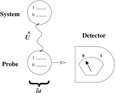
Figure 1: This is a schematic diagram of the type of model used in this paper. The system is a single two-level system, or q-bit. It interacts briefly with a probe q-bit over a time interval $\delta t$, and the probe bit is subsequently measured

The initial state of the system and probe can be written as a simple tensor product ${|\psi_{0}\rangle}_{s}\otimes{|\phi_{0}\rangle}_{p}$. After the system and probe have interacted, however, the new joint state ${|\Psi\rangle}$ will generally no longer be a product. A state of this type, which cannot be written as a product, is said to be entangled. Such states have many curious properties, without classical analogues.

Even though the joint state ${|\Psi\rangle}$ is pure, we cannot describe either the system or the probe alone by a pure state. It is possible, however, to describe them by a mixed state, by finding the reduced density operator. The reduced density operator $\rho_{s}$ for the system is found by taking a partial trace of the joint state over the probe degree of freedom:

$$\rho_{s}={\rm Tr}_{p}\{{|\Psi\rangle}{\langle\Psi|}\}\;.$$ (13)

This mixed state $\rho_{s}$ gives exactly the same predictions as the joint state ${|\Psi\rangle}$ for any measurement which is restricted to the system alone. We can, of course, find a similar reduced density matrix $\rho_{p}$ for the probe by taking a partial trace over the system.

Provided that the joint state ${|\Psi\rangle}$ is pure, the mixed states $\rho_{s}$ and $\rho_{p}$ must have the same von Neumann entropy: $S(\rho_{s})=S(\rho_{p})$. (This is true in general, not just for q-bits.) Because this quantity is the same whichever subsystem we trace out, and because it vanishes for product states, it is widely used as a measure of entanglement for pure states: the entropy of entanglement, $S_{E}({|\Psi\rangle})$.

Suppose now that our system and probe have interacted and are in an entangled state ${|\Psi\rangle}$. What happens if we measure the probe? As mentioned above, the measurement is represented by the two projection operators ${\hat{\cal P}}_{\pm}$ which sum to the identity ${\hat{\cal P}}_{+}+{\hat{\cal P}}_{-}={\hat{1}}$. Because these are projectors onto a two-dimensional Hilbert space, each of them projects onto a one-dimensional subspace. We can therefore write them as ${\hat{\cal P}}_{+}={|+\rangle}{\langle+|}$, ${\hat{\cal P}}_{-}={|-\rangle}{\langle-|}$. After allowing the system and probe to interact, and then measuring the probe, the system and probe will be in one of two possible joint states:

$$({\hat{1}}\otimes{\hat{\cal P}}_{\pm}){|\Psi\rangle} = ({\hat{1}}\otimes{\hat{\cal P}}_{\pm}){\hat{U}}{|\psi_{0}\rangle}\otimes{|\phi_{0}\rangle}$$ (14)

$$= {\hat{A}}_{\pm}{|\psi_{0}\rangle}\otimes{|\pm\rangle}\;,$$ (15)

(where we have not renormalized the final state). The system and probe are once more in a product state. The operators ${\hat{A}}_{\pm}$ are determined by the unitary transformation ${\hat{U}}$ and the initial state of the probe ${|\phi_{0}\rangle}$. The probabilities of the two outcomes are

$$p_{\pm} = ({\langle\psi_{0}|}\otimes{\langle\phi_{0}|}){\hat{U}}^{\dagger}({\hat{1}}\otimes{\hat{\cal P}}_{\pm}){\hat{U}}({|\psi_{0}\rangle}\otimes{|\phi_{0}\rangle})$$ (16)

$$= {\langle\psi_{0}|}{\hat{A}^{\dagger}}_{\pm}{\hat{A}}_{\pm}{|\psi_{0}\rangle}\;.$$ (17)

The fact that these two probabilities must add to 1 for any state ${|\psi_{0}\rangle}$ implies that ${\hat{A}^{\dagger}}_{+}{\hat{A}}_{+}+{\hat{A}^{\dagger}}_{-}{\hat{A}}_{-}={\hat{1}}$.

If we discard the probe after the measurement and renormalize the state, the system is left in the new state ${\hat{A}}_{\pm}{|\psi_{0}\rangle}/\sqrt{p_{\pm}}$. This is quite similar to the effects of a projective measurement; indeed, if ${\hat{A}}_{\pm}$ are projectors, this reduces to the usual formula for a projective measurement. Because of this, and because we are indirectly acquiring information about the system by measuring the probe, this is commonly referred to as a generalized measurement.

How much information is gained in such a generalized measurement? We can calculate this in exactly the same way as for a projective measurement. The Shannon entropy of the generalized measurement is $-p_{+}\log_{2}p_{+}-p_{-}\log_{2}p_{-}$. This must obviously be greater than the entropy of entanglement $S_{E}({|\Psi\rangle})$. We can choose projectors ${\hat{\cal P}}_{\pm}$ to minimize the Shannon entropy by writing the state ${|\Psi\rangle}$ in Schmidt form:

$${|\Psi\rangle}=\sqrt{p_{+}}{|+\rangle}_{s}\otimes{|+\rangle}_{p}+\sqrt{p_{-}}{|-\rangle}_{s}\otimes{|-\rangle}_{p}\;.$$ (18)

Choosing the right Schmidt bases ${|\pm\rangle}_{s,p}$ requires us to know the initial states ${|\psi_{0}\rangle}$ and ${|\phi_{0}\rangle}$ and the unitary transformation ${\hat{U}}$.

Of course, in the case described above, the system starts and ends in a pure state; so this generalized measurement also generates randomness. However, it is certainly capable of giving information about the system. Suppose that the initial state of the system is maximally mixed: $\rho_{s}={\hat{1}}/2$, with $S(\rho_{s})=1$. If we have it interact with the probe and carry out the measurement, then with probabilities

$$p_{\pm}={\rm Tr}\{{\hat{A}}_{\pm}\rho_{s}{\hat{A}^{\dagger}}_{\pm}\}$$ (19)

the system will be left in one of the states

$$\rho_{\pm}={\hat{A}}_{\pm}\rho_{s}{\hat{A}^{\dagger}}_{\pm}/p_{\pm}={\hat{A}}_{\pm}{\hat{A}^{\dagger}}_{\pm}/2p_{\pm}\;.$$ (20)

In general, neither of these states will be maximally mixed. The entropy of the system will be diminished by an average amount

$$\Delta S=1-p_{+}S(\rho_{+})-p_{-}S(\rho_{-})\;.$$ (21)

This represents the actual information gained about the system. This must always be less than or equal to the Shannon entropy of the generalized measurement, $-p_{+}\log_{2}p_{+}-p_{-}\log_{2}p_{-}$.

Let’s look at a couple of examples to see how this works. Suppose the system is initially in the maximally mixed state $\rho_{s}={\hat{1}}/2$; the probe is in the pure state ${|\phi_{0}\rangle}={|0\rangle}$; and we measure the probe using projectors onto the states $\{{|0\rangle},{|1\rangle}\}$. We let the interaction ${\hat{U}}$ be the CNOT gate from (7). In this case, we gain exactly 1 bit of information about the system, equal to the Shannon entropy of the measurement, and leaving the system in a pure state ${|0\rangle}$ or ${|1\rangle}$.

Suppose that we keep the same initial states and interaction, but instead make the measurement given by ${\hat{\cal P}}_{\pm}={|\pm\rangle}{\langle\pm|}$ where ${|\pm\rangle}=({|0\rangle}\pm{|1\rangle})/\sqrt{2}$. In this case, the Shannon entropy is still 1 bit, but we now gain no information about the system; it is left in exactly the same state as it started, the maximally mixed state $\rho_{s}={\hat{1}}/2$.

If we further generalize this scheme and allow the initial state of the probe to be mixed, then it is actually possible to lose information about the system; $\Delta S$ can be negative. For instance, an initial pure state for the system can become mixed, due to noise from interacting with a mixed environment.

With this very simple model of a quantum process, we can build up everything we need to understand both decoherence and quantum trajectories. We examine them both in the next two sections.

4 Decoherence

In discussing quantum evolution it is usually assumed that the quantum system is very well isolated from the rest of the world. This is a useful idealization, but it is rarely realized in practice, even in the laboratory. In fact, most systems interact at least weakly with external degrees of freedom Zurek ; Joos . This is the process of decoherence.

One way of taking this into account is to include a model of these external degrees of freedom in our description. Let us assume that in addition to the system in state ${|\psi\rangle}\in{\cal H}_{S}$ there is an external environment in state ${|E\rangle}\in{\cal H}_{E}$.

Systems which interact with their environments are said to be open. Most real physical environments are extremely complicated, and the interactions between systems and environments are often poorly understood. In analyzing open systems, one often makes the approximation of assuming a simple, analytically solvable form for the environment degrees of freedom.

For this paper, I will assume that both the system and the environment consist solely of q-bits. I will also assume a simple form of interaction, namely that the system q-bit interacts with one environment q-bit at a time, and that after interacting they never come into contact again; and that the environment q-bits have no Hamiltonian of their own. This may seem ridiculously oversimplified, but in fact it suffices to demonstrate most of the physics exhibited by much more realistic descriptions.

For this type of model, the Hilbert space of the system is ${\cal H}_{2}$ and the Hilbert space of the environment is ${\cal H}_{E}={\cal H}_{2}\otimes{\cal H}_{2}\otimes\cdots$. I will assume that all the environment q-bits start in some pure initial state ${|\phi_{0}\rangle}$, usually ${|0\rangle}$, though further elaborations of the model could include other pure-state and mixed-state environments. These environment q-bits play a role exactly like the probe in section 3, except that they are never measured.

We can describe this as an effective process on the system alone. After each interaction, the system’s reduced state $\rho$ undergoes the evolution

$$\rho\rightarrow\sum_{k=\pm}{\hat{A}}_{k}\rho{\hat{A}^{\dagger}}_{k}\;,$$ (22)

so that after $t$ steps the state becomes

$$\rho(t)=\sum_{k_{1},\ldots,k_{t}=\pm}{\hat{A}}_{k_{t}}\cdots{\hat{A}}_{k_{1}}\rho(0){\hat{A}^{\dagger}}_{k_{1}}\cdots{\hat{A}^{\dagger}}_{k_{t}}\;.$$ (23)

The operators ${\hat{A}}_{\pm}$ depend on the choice of ${\hat{U}}$ and ${|\phi_{0}\rangle}$; they are determined just as in the generalized measurement case described in section 3. However, this determination is not unique; many choices of ${\hat{A}}_{k}$ yield the same process (22).

An interesting case is when the interaction ${\hat{U}}$ is weak, that is, close to the identity:

$${\hat{U}}=\exp(-i\epsilon{\hat{H}})\approx{\hat{1}}-i\epsilon{\hat{H}}-(\epsilon{\hat{H}})^{2}/2\;,$$ (24)

where $|{\hat{H}}|\sim O(1),|\epsilon|\ll 1,{\hat{H}}={\hat{H}}^{\dagger}$. If the environment q-bits arrive with an average separation of $\delta t$, and $\epsilon$ is sufficiently small, then the system state $\rho$ will approximately obey a continuous evolution equation

$${d\rho\over dt}=-i[{\hat{H}}_{\rm eff},\rho]+{\hat{L}}\rho{\hat{L}^{\dagger}}-(1/2){\hat{L}^{\dagger}}{\hat{L}}\rho-(1/2)\rho{\hat{L}^{\dagger}}{\hat{L}}\;.$$ (25)

This is a Lindblad master equation Lindblad . In terms of ${\hat{H}}$, ${\hat{H}}_{\rm eff}\propto{\langle\phi_{0}|}{\hat{H}}{|\phi_{0}\rangle}$, and ${\hat{L}}\propto{\langle\bar{\phi_{0}}|}{\hat{H}}{|\phi_{0}\rangle}$.

Let’s consider a concrete example. Suppose the interaction is ${\hat{U}}=\exp(-i\epsilon{\hat{H}})$ with ${\hat{H}}={\hat{\sigma}_{z}}\otimes{\hat{\sigma}_{x}}$, and the environment bits are initially in state ${|0\rangle}$. Then the reduced density matrix for the system alone will obey (25) with ${\hat{H}}_{\rm eff}=0$ and ${\hat{L}}=(\epsilon/\sqrt{\delta t}){\hat{\sigma}_{z}}$. This master equation will cause a system initially in the pure state $\alpha{|0\rangle}+\beta{|1\rangle}$ to evolve in the long time limit to the mixed state $\rho=|\alpha|^{2}{|0\rangle}{\langle 0|}+|\beta|^{2}{|1\rangle}{\langle 1|}$. As the system state becomes mixed, its von Neumann entropy grows, reflecting a gradual loss of information about the system, or (alternatively) a growing entanglement of the system with the environment. Different interactions or environment states of course will lead to different master equations.

5 Quantum trajectories

We can readily generalize our model of decoherence by supposing that we have experimental access to the q-bits of the environment. After each bit has interacted with the system, we measure it using some predefined projective measurement; based on the outcome of this measurement, we update our knowledge of the system state. The series of decohering interactions then becomes a series of generalized measurements, as described in section 3.

The evolution of the system state is no longer deterministic; it becomes stochastic due to the randomness of the measurement outcomes. We also now acquire information about the system as it is lost to the environment. Given perfect measurements of the environment, the system will remain always in a pure state.

Rather than the evolution (22), the system now undergoes

$${|\psi\rangle}\rightarrow{\hat{A}}_{\pm}{|\psi\rangle}/\sqrt{p_{\pm}}$$ (26)

with probabilities $p_{\pm}={\langle\psi|}{\hat{A}^{\dagger}}_{\pm}{\hat{A}}_{\pm}{|\psi\rangle}$. After $t$ steps, the state will have become

$${|\psi(t)\rangle}={\hat{A}}_{k_{t}}\cdots{\hat{A}}_{k_{1}}{|\psi(0)\rangle}/\sqrt{p_{k_{1},\ldots,k_{t}}}\;,$$ (27)

where the $k_{i}$ take the values $\pm$. Note that, while there was an ambiguity in ${\hat{A}}_{\pm}$ for our decoherence model, by choosing a particular measurement we fix a particular choice of ${\hat{A}}_{\pm}$.

This evolution becomes more interesting when the interaction is weak, as described in the previous section. In this case, our series of generalized measurements are weak measurements Vaidman – on average, they disturb the system state very little, but also give very little information. The effective evolution of the system becomes approximately continuous, but rather than a master equation, it is a stochastic Schrödinger equation.

Let us consider the same system described at the end of section 4, but now including a measurement of each environment q-bit after it has interacted with the system. After the interaction, the joint state of the system and environment bit is

$${\hat{U}}{|\psi\rangle}\otimes{|0\rangle}\approx(1-\epsilon^{2}/2){|\psi\rangle}\otimes{|0\rangle}-i\epsilon{\hat{\sigma}_{z}}{|\psi\rangle}\otimes{|1\rangle}\;.$$ (28)

Suppose that we measure the environment bit in the $\{{|0\rangle},{|1\rangle}\}$ basis. Then with probability $p_{0}\approx 1-\epsilon^{2}$ the bit will be found in state ${|0\rangle}$ and the system state will remain unchanged. With a small probability $p_{1}\approx\epsilon^{2}$, however, the environment bit will be found in state ${|1\rangle}$ and the state of the system will change to ${\hat{\sigma}_{z}}{|\psi\rangle}$. This type of evolution can be approximated as a quantum jump equation:

$${|d\psi\rangle}=({\hat{\sigma}_{z}}-{\hat{1}}){|\psi\rangle}dN\;,$$ (29)

where $dN$ is a stochastic differential variable which is 0 most of the time, but occasionally (with probability of $\epsilon^{2}$ in each interval $\delta t$) becomes 1. Writing this in terms of the statistical mean $M[\cdot]$,

$$dN^{2}=dN\;,\ \ \ M[dN]=(\epsilon^{2}/\delta t)dt\;.$$ (30)

Instead of the measurement above, we might instead measure the environment bits in the basis ${|\pm\rangle}=({|0\rangle}\pm{|1\rangle})/\sqrt{2}$. In terms of this basis, the joint state becomes

$${\hat{U}}{|\psi\rangle}\otimes{|0\rangle}={1\over\sqrt{2}}\exp(-i\epsilon{\hat{\sigma}_{z}}){|\psi\rangle}\otimes{|+\rangle}+{1\over\sqrt{2}}\exp(+i\epsilon{\hat{\sigma}_{z}}){|\psi\rangle}\otimes{|-\rangle}\;.$$ (31)

The system state undergoes one of two weak unitary transformations, based on the outcome of the measurement; the two outcomes have equal probability. This evolution is approximated by the continuous quantum state diffusion equation

$${|d\psi\rangle}=-i{\hat{L}}{|\psi\rangle}dW\;,$$ (32)

where ${\hat{L}}=(\epsilon/\sqrt{\delta t}){\hat{\sigma}_{z}}$ and $dW$ is a real differential stochastic variable obeying

$$M[dW]=0\;,M[dW^{2}]=dt\;.$$ (33)

We see how exactly the same physical system can exhibit two very different-looking evolutions based on the choice of environmental measurement. In both cases, if we average over all possible trajectories we recover the solution of the master equation (25):

$$M[{|\psi(t)\rangle}{\langle\psi(t)|}]=\rho(t)\;.$$ (34)

Because of this, these different stochastic Schrödinger equations are often referred to as different unravelings of the master equation.

6 Quantum trajectories and decoherent histories

As is clear from the previous sections, the formalism of quantum trajectories calls on nothing more than standard quantum mechanics, and as framed above is in no way an alternative theory or interpretation. Everything can be described solely in terms of measurements and unitary transformations, the building blocks of the usual Copenhagen interpretation.

However, many people have expressed dissatisfaction with the standard interpretation over the years, usually due to the role of measurement as a fundamental building block of the theory. Measuring devices are large, complicated things, very far from elementary objects; what exactly constitutes a measurement is never defined; and the use of classical mechanics to describe the states of measurement devices is not justified. Presumably the individual atoms, electrons, photons, etc., which make up a detector can themselves be described by quantum mechanics. If this is carried to its logical conclusion, however, and a Schrödinger equation is constructed for the measurement process, one obtains not classical behavior, but rather giant macroscopic superpositions such as the famous Schrödinger’s cat paradox Schroedinger .

One approach to this problem is to retain the usual quantum theory, but to eliminate measurement as a fundamental concept, finding some other interpretation for the predicted probabilities. While many interpretations follow this approach, the one that is most closely tied to quantum trajectories is the decoherent (or consistent) histories formalism of Griffiths, Omnés, Gell-Mann and Hartle Griffiths ; Omnes ; GellMann . In this formalism, probabilities are assigned to histories of events rather than measurement outcomes at a single time. These can be grouped into sets of mutually exclusive, exhaustive histories whose probabilities sum to 1. However, not all histories can be assigned probabilities under this interpretation; only histories which lie in sets which are consistent, that is, whose histories do not exhibit interference with each other, and hence obey the usual classical probability sum rules.

Each set is basically a choice of description for the quantum system. For the models considered in this paper, the quantum trajectories correspond to histories in such a consistent set. The probabilities of the histories in the set exactly equal the probabilities of the measurement outcomes corresponding to a given trajectory. This equivalence has been shown between quantum trajectories and consistent sets for certain more realistic systems, as well DGHP ; Brun2 ; Brun3 .

For a given quantum system, there can be multiple consistent descriptions which are incompatible with each other; that is, unlike in classical physics, these descriptions cannot be combined into a single, more finely-grained description. In quantum trajectories, different unravelings of the same evolution correspond to such incompatible descriptions. In both cases, this is an example of the complementarity of quantum mechanics.

We see, then, that while quantum trajectories can be straightforwardly defined in terms of standard quantum theory when the environment is subjected to repeated measurements, even in the absence of such measurements there is an interpretation of the trajectories in terms of decoherent histories. Because the consistency conditions guarantee that the probability sum rules are obeyed, one can therefore use quantum trajectories as a calculational tool even in cases where no actual measurements take place.

7 Conclusions

In this paper I have presented a simple model of a system and environment consisting solely of quantum bits, using no more than single-bit measurements and two-bit unitary transformations. The simplicity of this model makes it particularly suitable for demonstrating the properties of decoherence and quantum trajectories. We can quantify the transfer of information from system to environment, the amount of entanglement, and the randomness produced by particular choices of measurement.

Quantum trajectories can often simplify the description of an open quantum system in terms of a stochastically evolving pure state rather than a density matrix. While for the q-bit models of this paper there is no great advantage in doing so, for more complicated systems this can often make a tremendous practical difference Schack .

The ideas behind decoherence and quantum trajectories developed largely separately from the ideas which have led to the recent explosion of interest in quantum information; but I would argue that both areas can contribute much to the understanding of the other. I hope that this paper has given support to this view.

References

- (1) W.H. Zurek: Phys. Rev. D 24, 1516 (1981); Phys. Rev. D 26, 1862 (1982); Physics Today 44, 36 (1991)
- (2) E. Joos, H.D. Zeh: Z. Phys. B 59, 229 (1985)
- (3) H.J. Carmichael: An Open Systems Approach to Quantum Optics (Springer, Berlin, 1993).
- (4) J. Dalibard, Y. Castin, K. Mølmer: Phys. Rev. Lett. 68, 580 (1992)
- (5) R. Dum, P. Zoller, H. Ritsch: Phys. Rev. A 45, 4879 (1992)
- (6) C.W. Gardiner, A.S. Parkins, P. Zoller: Phys. Rev. A 46, 4363 (1992)
- (7) N. Gisin: Phys. Rev. Lett. 52, 1657 (1984); Helv. Phys. Acta. 62, 363 (1989)
- (8) L. Diósi: J. Phys. A 21, 2885 (1988); Phys. Lett. 129A, 419 (1988); Phys. Lett. 132A, 233 (1988)
- (9) N. Gisin, I.C. Percival: J. Phys. A 25, 5677 (1992); J. Phys. A 26, 2233, 2245 (1993)
- (10) R. Schack, T.A. Brun, I.C. Percival: J. Phys. A 28, 5401 (1995)
- (11) M.A. Nielsen, I.L. Chuang: Quantum Computation and Quantum Information (Cambridge University Press, Cambridge, 2000)
- (12) T.A. Brun: Am. J. Phys. 70, 719–737 (2002)
- (13) L. Vaidman, in: Advances in quantum phenomena, ed. by E.G. Beltrametti, J.-M. Levy-Leblond (Plenum Press, 1995) p.357
- (14) G. Lindblad: Commun. Math. Phys. 48, 119 (1976)
- (15) E. Schrödinger: Naturwissenschaften 23, 807, 823, 844 (1935)
- (16) R.B. Griffiths: J. Stat. Phys. 36, 219 (1984); Phys. Rev. A 54, 2759 (1996); ibid. 57, 1604 (1998)
- (17) R. Omnès: The Interpretation of Quantum Mechanics (Princeton University Press, Princeton, 1994); Understanding Quantum Mechanics (Princeton University Press, Princeton, 1999)
- (18) M. Gell-Mann, J.B. Hartle, in: Complexity, Entropy, and the Physics of Information, SFI Studies in the Science of Complexity v. VIII ed. by W. Zurek (Addison-Wesley, Reading, 1990) p.425; in: Proceedings of the Third International Symposium on the Foundations of Quantum Mechanics in the Light of New Technology, ed. by S. Kobayashi, H. Ezawa, Y. Murayama, S. Nomura (Physical Society of Japan, Tokyo, 1990) p.321; in: Proceedings of the 25th International Conference on High Energy Physics, Singapore, 2–8 August 1990, ed. by K.K. Phua, Y. Yamaguchi (World Scientific, Singapore, 1990)
- (19) L. Diósi, N. Gisin, J.J. Halliwell, I.C. Percival: Phys. Rev. Lett. 21, 203 (1995)
- (20) T.A. Brun: Phys. Rev. Lett. 78, 1833 (1997)
- (21) T.A. Brun: Phys. Rev. A 61, 042107 (2000)