PLAYING PRISONER’S DILEMMA WITH QUANTUM RULES

Abstract

Quantum game theory is a recently developing field of physical research. In this paper, we investigate quantum games in a systematic way. With the famous instance of the Prisoner’s Dilemma, we present the fascinating properties of quantum games in different conditions, i.e. different number of the players, different strategic space of the players and different amount of the entanglement involved.

1 Introduction

Game theory is a distinct and interdisciplinary approach to the study of human behavior. The foundation of modern game theory can be traced back to the mathematician John Von Neumann who, in collaboration with the mathematical economist Oskar Morgenstern, wrote the mile stone book Theory of Games and Economic Behavior[1]. Game theory has since become one of the most important and useful tools for a wide range of research from the economics, social science to biological evolution[2].

However, game theory is now being developed in a completely new way. It is extended into the quantum realm by physicists interested in quantum information theory[3]. In quantum game theory, the players play the game abiding by quantum rules. Therefore, the primary results of quantum games are very different from those of their classical counterparts[4, 5, 6, 7, 8, 9, 10, 11, 12, 13, 14]. For example, in an otherwise fair zero-sum coin toss game, a quantum player can always win against his classical opponent if he adopts quantum strategies[4, 5]. In some other original dilemma games, problems can be resolved by playing with quantum rules[6, 7, 8, 12, 14]. Besides the theoretical research on quantum games, a quantum game has been experimentally realized on a NMR quantum computer[10, 15].

In this paper, we investigate quantum games in a systematic way. For the particular case of the quantum Prisoner’s Dilemma, we investigate this quantum game in different conditions. These conditions differ in the number of players, the strategic space and the role of entanglement in the quantum game. It is shown that the properties of the quantum game can change fascinatingly with the variations of the game’s conditions.

2 Quantum Games

In the remaining part of this paper, we take a detailed investigation of quantum games with the particular case of the Prisoner’s Dilemma. Firstly, we present the two-player Prisoner’s Dilemma which has been presented in [6]. Secondly, we investigate the three-player Prisoner’s Dilemma. In the following discussions the organization is as follows: (i) the classical version of the game, (ii) the quantization scheme, and (iii) the investigation of the game with different strategic spaces.

2.1 Two-player prisoner’s dilemma

Table 1: The payoff table for the Prisoners’ Dilemma.

	Bob: $C$	Bob: $D$
Alice: $C$	$\left(3,3\right)$	$\left(0,5\right)$
Alice: $D$	$\left(5,0\right)$	$\left(1,1\right)$

The publication of Theory of Games and Economic Behavior was a particularly important step in the development of game theory. But in some ways, Tucker’s proposal of the problem of the Prisoners’ Dilemma was even more important. This problem, which can be stated in one page, could be the most influential one in the social sciences in the later half of the twentieth century. The name of the Prisoner’s Dilemma arises from the following scenario: two burglars, Alice and Bob are caught by the police and are interrogated in separate cells, without no communication between them. Unfortunately, the police lacks enough admissible evidence to get a jury to convict. The chief inspector now makes the following offer to each prisoner: If one of them confess to the robbery, but the other does not, then the former will get unit reward of 5 units and the latter will get nothing. If both of them confess, then each get 1 unit as a reward. If neither of them confess, then each will get payoff 3. Since confession means a “defect” strategy and no confession means “cooperate” with the other player, the classical strategies of the players are thus denoted by “$D$” and “$C$”, respectively. Table 1 indicates the payoffs of Alice and Bob according to their strategies.

From Table 1, we see that $D$ is the dominant strategy of the game. Since the players are rational and care only about their individual payoffs, both of them will resort to the dominant strategy $D$ and get payoff $1$. In terms of game theory, $(D,D)$ is a dominant strategy equilibrium. However, this dominant strategy equilibrium is inferior to the Pareto Optimal $(C,C)$, which yields payoff 3 to each players. This is the catch of the Prisoner’s Dilemma.

2.1.1 Quantization scheme

Figure 1: The setup of two-player quantum games.

Recently, this famous game got a new twist: It is studied in the quantum world by physicists[6, 7]. By allowing the players to adopt quantum strategies, it is interesting to find that the original dilemma in the classical version of this game could be removed. The physical model of this quantum game is illustrated in Fig 1. Different from the classical game, each player has a qubit and can manipulate it independently (locally) in the quantum version of this game. The quantum formulation proceeds by assigning the possible outcomes of the classical strategies $C$ and $D$ the two basis vectors of a qubit, denoted by

$$\left|C\right\rangle=\left(\begin{array}[]{c}1\\ 0\end{array}\right),\left|D\right\rangle=\left(\begin{array}[]{c}0\\ 1\end{array}\right).$$ (1)

The gate

$$\hat{J}=\exp\left\{i\gamma\hat{D}\otimes\hat{D}/2\right\},$$ (2)

with $0\leqslant\gamma\leqslant\pi/2$, can be considered as a gate which produce entanglement between the two qubits. The game started from the pure state $\left|CC\right\rangle$. After passing through the gate $\hat{J}$, the game’s initial state is

$$\left|\psi_{i}\right\rangle=\widehat{J}\left|CC\right\rangle=\cos\frac{\gamma}{2}\left|CC\right\rangle+i\sin\frac{\gamma}{2}\left|DD\right\rangle.$$ (3)

Since the entropy (entanglement) of $\left|\psi_{i}\right\rangle$ is

$$S=-\sin^{2}\frac{\gamma}{2}\ln\sin^{2}\frac{\gamma}{2}-\cos^{2}\frac{\gamma}{2}\ln\cos^{2}\frac{\gamma}{2},$$ (4)

the parameter $\gamma$ can be reasonably considered as a measure of the game’s entanglement.

After the initial state was produced, each player apply a unitary operation on his/her individual qubit. Later on, the game’s state goes through $\hat{J}^{{\dagger}}$ and the final state is $\left|\psi_{f}\right\rangle$. According to the corresponding entry of the payoff table (Table 1), the explicit expressions of both player’s payoff functions can be written as follows:

$$\$_{A} = 3P_{CC}+1P_{DD}+5P_{DC}+0P_{CD},$$

$$\$_{B} = 3P_{CC}+1P_{DD}+0P_{DC}+5P_{CD},$$ (5)

where $\$_{A}$ ($\$_{B}$) represents Alice’s (Bob’s) payoff and $P_{\sigma\sigma^{\prime}}=\left|\left\langle\sigma\sigma^{\prime}\right|\left.\psi_{f}\right\rangle\right|^{2}$ is the probability that the final state will collapse into $\left|\sigma\sigma^{\prime}\right\rangle$. At the end of the game, each player will get a reward according the payoff function.

In the following subsections, we investigate this quantum game with different strategic spaces. It is interesting to find that the game’s property does not necessarily become better with the extension of the strategic space.

2.1.2 Restricted strategic space

In this section, we will focus on the restricted strategic space situation, i.e. a two parameter strategy set which is a subset of the whole unitary space[6]. The explicit expression of the operator is given by

$$U(\theta,\phi)=\left(\begin{array}[]{cc}e^{i\phi}\cos\frac{\theta}{2}&\sin\frac{\theta}{2}\\ -\sin\frac{\theta}{2}&e^{-i\phi}\cos\frac{\theta}{2}\end{array}\right),$$ (6)

where $0\leqslant\theta\leqslant\pi$ and $0\leqslant\phi\leqslant\pi/2$. We can see that

$$U(0,0)=\left(\begin{array}[]{cc}1&0\\ 0&1\end{array}\right)$$ (7)

is the identity operator and

$$U(\pi,0)=\left(\begin{array}[]{cc}0&1\\ -1&0\end{array}\right)$$ (8)

is somehow equivalent to a bit-flip operator. The former corresponds to the classical “cooperation” strategy and the latter to “defect”.

This situation has been investigated in details by Eisert et al.[6]. Here, we present the main results of their work: (i) For a separable game with $\gamma=0$, there exists a pair of quantum strategies $\hat{D}\otimes\hat{D}$, which is the Nash equilibrium and yields payoff $\left(1,1\right)$. Indeed, this quantum game behaves “classically”, i.e. the Nash equilibrium for the game and the final payoffs for the players are the same as in the classical game. So the separable game does not display any features which go beyond the classical game. (ii) For a maximally entangled quantum game with $\gamma=\pi/2$, there exists a pair of strategies $\hat{Q}\otimes\hat{Q}$, which is a Nash equilibrium and yields payoff $\left(3,3\right)$, having the property to be the Pareto optimal. Therefore the dilemma that exists in the classical game is removed.

In the quantum game, we can see that in the decision-making step the player has means of communication with each other, i.e. no one has any information about which strategy the other player will adopt. This is the same as in classical game. Hence, it is natural to ask why the dilemma game shows such a fascinating property in quantum game? The answer is entanglement, the key to the quantum information and quantum computation[16, 17]. Although there is no communication between the two players, the two qubits are entangled, and therefore one player’s local action on his qubit will affect the state of the other. Entanglement plays as a contract of the game.

In the Eisert et al.’s scheme, the dilemma was removed when the game’s state is maximal entangled. It is also interesting to investigate the game’s behavior when the amount of entanglement varies. In one of our previous works[7], we find that there exist two thresholds of the game’s entanglement, $\gamma_{th1}=\arcsin\sqrt{1/5}$ and $\gamma_{th2}=\arcsin\sqrt{2/5}$. In different domains of entanglement, the quantum game shows different properties. For $0\leqslant\gamma\leqslant\gamma_{th1}$ , the quantum game behaves classically, i.e. the Nash equilibrium of the game is $\hat{D}\otimes\hat{D}$ and the final payoff for the players are both $1$, which are the same as the classical version of this game. Hence,the quantum game does not display any features which go beyond the classical game for the small amount of entanglement of the game’s state. For $\gamma_{th1}\leqslant 0\leqslant\gamma_{th2}$, the games shows some novel features which has no classical analog. In this domain, $\hat{D}\otimes\hat{D}$ is no longer Nash equilibrium of the game. However, there are two new Nash Equilibria, $\hat{D}\otimes\hat{Q}$ and $\hat{Q}\otimes\hat{D}$. The payoff to the one who resorts to strategy $\hat{D}$ is $5\cos^{2}\gamma$ and to the other adopting $\hat{Q}$ is $5\sin^{2}\gamma$. Since $5\cos^{2}\gamma\geqslant 5\sin^{2}\gamma$ for $\gamma_{th1}\leqslant\gamma\leqslant\gamma_{th2}$, the one choosing strategy $\hat{D}$ is better rewarded. Note that the physical structure of the game is symmetric with respect to the interchange of the two players. However, both Nash equilibrium $\hat{D}\otimes\hat{Q}$ and $\hat{Q}\otimes\hat{D}$ cause the the unfairness of the game. We think that there are two reasons for the asymmetry situation: (i) Since the definition of Nash equilibrium allows multiple Nash Equilibria to coexist, the solutions may be degenerate. Therefore the definition itself allows the possibility of such an asymmetry. This situation is similar to the spontaneous symmetry breaking; (ii) If we consider the two Nash Equilibria as a whole, they are fully equivalent and the game remains symmetric. But finally, the two players have to choose one from the two equilibria. This also causes the asymmetry of the game. For $\gamma_{th2}\leqslant\gamma\leqslant\pi/2$, the game shows exciting features. A novel Nash equilibrium $\hat{Q}\otimes\hat{Q}$ arises with $\$_{A}(\hat{Q},\hat{Q})=\$_{B}(\hat{Q},\hat{Q})=3$, which satisfies the property of Pareto Optimal. Therefore, as long as the the amount of entanglement exceeds a certain threshold, the dilemma can be removed.

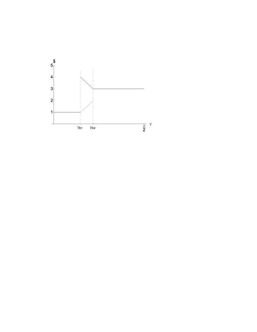
Figure 2: The expected payoff for Alice as a function of the measure of the parameter $\gamma$ when both players resort to Nash Equilibrium. For $\gamma_{th1}<\gamma<\gamma_{th2}$, the dash line and the dot line represent Alice’s payoff when the Nash Equilibrium is $\hat{D}\otimes\hat{Q}$ and $\hat{Q}\otimes\hat{D}$ respectively.

Fig 2 illustrates Alice’s payoff as a function of the parameter $\gamma$ when both players resort to Nash equilibrium. From this figure, we observe that the game’s property depends discontinuously on the amount of the entanglement. This discontinuity can be considered as entanglement correlated phase transition, i.e. the game can be considered to lie in three different phases. For $0\leqslant\gamma\leqslant\gamma_{th1}$, the game displays no advantage over classical game. So this domain can be considered as the classical phase. For $\gamma_{th1}\leqslant\gamma\leqslant\gamma_{th2}$, there are two Nash Equilibria for the game, both of which yield asymmetric payoffs to the players. This domain can be considered as the transitional phase from classical to quantum. For $\gamma_{th2}\leqslant\gamma\leqslant\pi/2$, a novel Nash equilibrium $\hat{Q}\otimes\hat{Q}$ appears with payoff $\left(3,3\right)$. This strategic profile has the property to be Pareto Optimal and hence the dilemma disappears, and this domain can be considered as the quantum phase.

One interesting thing should be pointed out is that if we change the numerical values in the payoff table (Table 1), Fig 2 will varies interestingly. If these numerical values satisfy some particular condition, the transition phase in which the game has two asymmetric Nash equilibria will disappear. Furthermore, the phase transition exhibit interesting variation with respect to the change of the numerical values in the payoff matrix, so does the property of the game. For different numerical values, the game may or may not have a transition phase, or even the classical and quantum phases can overlap and form a new phase, the coexistence phase. The detailed presentation can be found in [20].

2.1.3 General quantum operations

In a recent Letter, it was pointed out that restricting the strategic space of the players can not reflect any reasonable physical constraint because the set is not closed under composition[18]. The observation is that any operation of the restricted strategic space can consist of $\left\{\hat{I},\hat{\sigma}_{y},\hat{\sigma}_{z}\right\}$ with certain coefficients. $\hat{I}$ equivalent to $\hat{C}$ operation, $\hat{\sigma}_{y}$ to $\hat{D}$ and $\hat{\sigma}_{z}$ to $\hat{Q}$. Note that $\hat{\sigma}_{y}$ is an optimal strategy counter to $\hat{I}$. And similarly $\hat{\sigma}_{z}$ is the ideal counter-strategy to $\hat{\sigma}_{y}$. However, the best reply to strategy $\hat{\sigma}_{z}$, which is $\hat{\sigma}_{x}$, is not included in this restricted strategic space. Thus, the dilemma situation could be solved by applying $\hat{Q}\otimes\hat{Q}$. The general case is that the player should be permitted free choice of any unitary operations. If so, the operation $\hat{\sigma}_{x}$ counter to $\hat{\sigma}_{z}$ is permitted. The interesting observation is that $\hat{I}$ is the ideal counter-strategy if one’s opponent plays $\hat{\sigma}_{x}$. Then $\left\{\hat{I},\hat{\sigma}_{x},\hat{\sigma}_{y},\hat{\sigma}_{z}\right\}$ forms a inter-restricted cycle, and therefore if the amount of entanglement of the game’s state is maximal, there is no pure-strategy Nash equilibrium in this quantum game[18, 19]. However, the game remains to have mixed Nash equilibria[19].

As we have seen in the preceding section, properties of quantum games change fascinatingly when the amount of the game’s entanglement varies. So, assuming that the player could choose any strategy from the complete set of all local unitary operations, it is then natural to investigate whether there exists pure strategy Nash equilibrium for this game when the game is not maximally entangled. Here we show that as long as the game’s entanglement is below a certain boundary[7], the game has infinite number of pure Nash equilibria. While for entanglement beyond that boundary, the game behaves the same as in the maximally entangled case.

The general form of $2\times 2$ unitary matrix can be represented by Pauli matrices as following:

$$\hat{U}(w,x,y,z)=w\hat{I}+ix\cdot\hat{\sigma}_{x}+iy\cdot\hat{\sigma}_{y}+iz\cdot\hat{\sigma}_{z},$$ (9)

where all the coefficients $w$, $x$, $y$ and $z$ are real and satisfy the normalization condition

$$w^{2}+x^{2}+y^{2}+z^{2}=1.$$ (10)

We plot Alice’s payoff as a function of the parameter $\gamma$ when both players resort to Nash equilibrium in Fig 3. $\gamma_{B}=\arcsin\sqrt{1/3}$ is the boundary of the game’s entanglement. For $0\leqslant\gamma\leqslant\gamma_{B}$ , we find that there are infinite number of Nash equilibrium for any determined value of $\gamma$. But as long as the $\gamma$ is given, no matter which profile Nash equilibrium the players choose, the payoffs for both players are determined and are the same, which are $\$_{A}=$ $\$_{B}=1+2\sin^{2}\gamma$. It shows that the payoff of each player is a monotonous increasing function of $\gamma$. But if the entanglement of the game’s state exceeds the boundary $\gamma_{B}$, the game will have no pure strategy Nash equilibrium. So we have shown that if the strategic space of the players is all of $SU\left(2\right)$, the entanglement could still enhance the property of this quantum game.

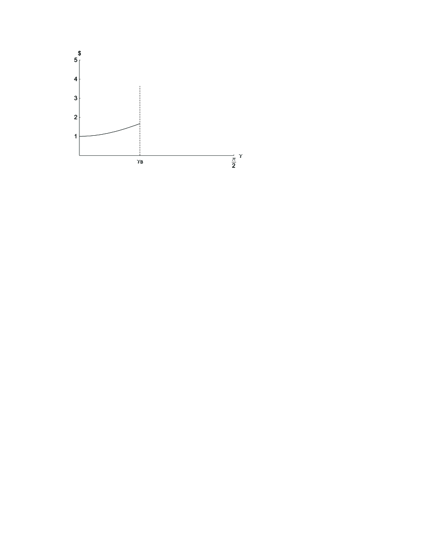
Figure 3: The expected payoff for Alice as a function of the measure of the parameter $\gamma$ when both players resort to Nash Equilibrium.

2.2 Multiplayer quantum games

The effect of “two’s company, three’s a crowd” is quite familiar in physical world[11]. Complex phenomenon tends to emerge in multipartite systems. Hence, to investigate multiplayer quantum games in multi-qubit system will be more interesting and significant. Recently, quantum games with more than two players was firstly investigated and such games can exhibit certain forms of pure quantum equilibrium that have no analog in classical games, or even in two player quantum games[12, 21]. In the following discussion, we investigate multiplayer quantum games with the particular case of the three-player Prisoner’s Dilemma. Since the structure of the game is symmetric, and for more explicit expression, our investigation focus on the symmetric solution of the game. In this case, we will show that the quantum game can display miscellaneous qualities under different conditions. At first, let’s extend the two-player Prisoner’s Dilemma to the three-player case.

2.2.1 Three-player prisoner’s dilemma

The scenario of the three player Prisoners’ Dilemma is similar to the two-player situation[1]. Besides Alice and Bob, a third player, Colin joins this game. They are picked up by the police and interrogated in separate cells without a chance to communicate with each other. For the purpose of this game, it makes no difference whether or not Alice, Bob or Colin actually committed the crime. The players are told the same thing: If they all choose strategy $D$ (defect), each of them will get payoff $1$; if the players all resort to strategy $C$ (cooperate), each of them will get payoff $3$; if one of the players choose $D$ but the other two do not, $5$ is payoff for the former and $2$ for the latter two; if one of the players choose $C$ while the other two adopt $D$, $0$ is payoff for the former and $4$ for the latter two.

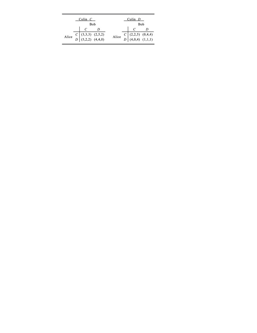
Figure 4: The payoff Table of the 3-player Prisoners’ Dilemma. The first entry in the parenthesis denotes the payoff of Alice, the second number denotes the payoff of Bob, and the third number denotes the payoff of Colin.

Fig 4 indicates the payoffs of the three players depending on their decisions. The game is symmetric for the three players, and the strategy $D$ dominates strategy $C$ for all of them. Since the selfish players all choose $D$ as optimal strategy, the unique Nash equilibrium is $(D,D,D)$ with payoff $(1,1,1)$. This is a Pareto inferior outcome, since $(C,C,C)$ with payoffs $(3,3,3)$ would be better for all three players. Optimizing the outcome for a subsystem will in general not optimize the outcome for the system as a whole. This situation is the very catch of the dilemma and the same as the two-player version of this game.

2.2.2 Quantization scheme

Our physical model for quantizing this game is similar as in [12] — see Fig 5. Just like the quantization scheme of the two-player Prisoner’s Dilemma, here we send each player a two state system or a qubit and they can locally manipulate their individual qubit. The possible outcomes of the classical strategies “Cooperate” and “Defect” are assigned to two basis vector

$$\left|0\right\rangle=\left(\begin{array}[]{c}1\\ 0\end{array}\right),\left|1\right\rangle=\left(\begin{array}[]{c}0\\ 1\end{array}\right)$$ (11)

in the Hilbert space. In the procedure of the game, its state is described by a vector in the tensor product space which is spanned by the eight classical basis $\left|\sigma\sigma^{{}^{\prime}}\sigma^{{}^{\prime\prime}}\right\rangle$ ( $\sigma,\sigma^{{}^{\prime}},\sigma^{{}^{\prime\prime}}\in\left\{0,1\right\}$), where the first, second and third entries belonging to Alice, Bob and Colin, respectively. At the beginning of the game the game’s state is $\left|000\right\rangle$. After the unitary transformation $J$, the initial state of the game is

$$\left|\psi_{i}\right\rangle=\hat{J}\left|000\right\rangle,$$ (12)

where

$$\hat{J}=\exp\left\{i\frac{\gamma}{2}\sigma_{x}\otimes\sigma_{x}\otimes\sigma_{x}\right\},$$ (13)

with $0\leqslant\gamma\leqslant\pi/2$, is the entangling gate of the game and is known to all of the players. Strategic move of Alice (Bob or Colin) is denoted by unitary operator $\hat{U}_{A}$ ($\hat{U}_{B}$ or $\hat{U}_{C}$), which are chosen from a certain strategic space $S$. Since the strategic moves of different players are independent, one player’s operator just operates on his individual qubit. After the operations of the players, the final state of the game prior to the measurement is give by

$$\left|\psi_{f}\right\rangle = \left|\psi_{f}\left(\hat{U}_{A},\hat{U}_{B},\hat{U}_{C}\right)\right\rangle$$ (14)

$$= \hat{J}^{{\dagger}}\left(\hat{U}_{A}\otimes\hat{U}_{B}\otimes\hat{U}_{C}\right)\hat{J}\left|000\right\rangle.$$

Hence, the final state of the game can be represented by density matrix

$$\rho_{f}=\left|\psi_{f}\right\rangle\left\langle\psi_{f}\right|.$$

Here, we will use the density matrix to get the final payoff for the players. This final state go forward to the subsequent measurement instrument and the players can get a reward according to their individual payoff operators. The payoff operators can be directly given from the corresponding entries of payoff matrix. For example, the payoff operator of Alice can be written as

$$\hat{\$}_{A} = 5\left|100\right\rangle\left\langle 100\right|+4\left(\left|110\right\rangle\left\langle 110\right|+\left|101\right\rangle\left\langle 101\right|\right)$$ (15)

$$+3\left|000\right\rangle\left\langle 000\right|+2\left(\left|001\right\rangle\left\langle 001\right|+\left|010\right\rangle\left\langle 010\right|\right)$$

$$+1\left|111\right\rangle\left\langle 111\right|+0\left|011\right\rangle\left\langle 011\right|.$$

Hence the expectation value of Alice’s payoff is given by

$$\$_{A}\left(U_{A},U_{B},U_{C}\right)=tr\left[\hat{\$}_{A}\rho_{f}\right].$$ (16)

Since the game is symmetric for three players, the payoff functions of Bob and Colin can also be obtained directly from the same analyzing together with the payoff matrix (see Fig 4).

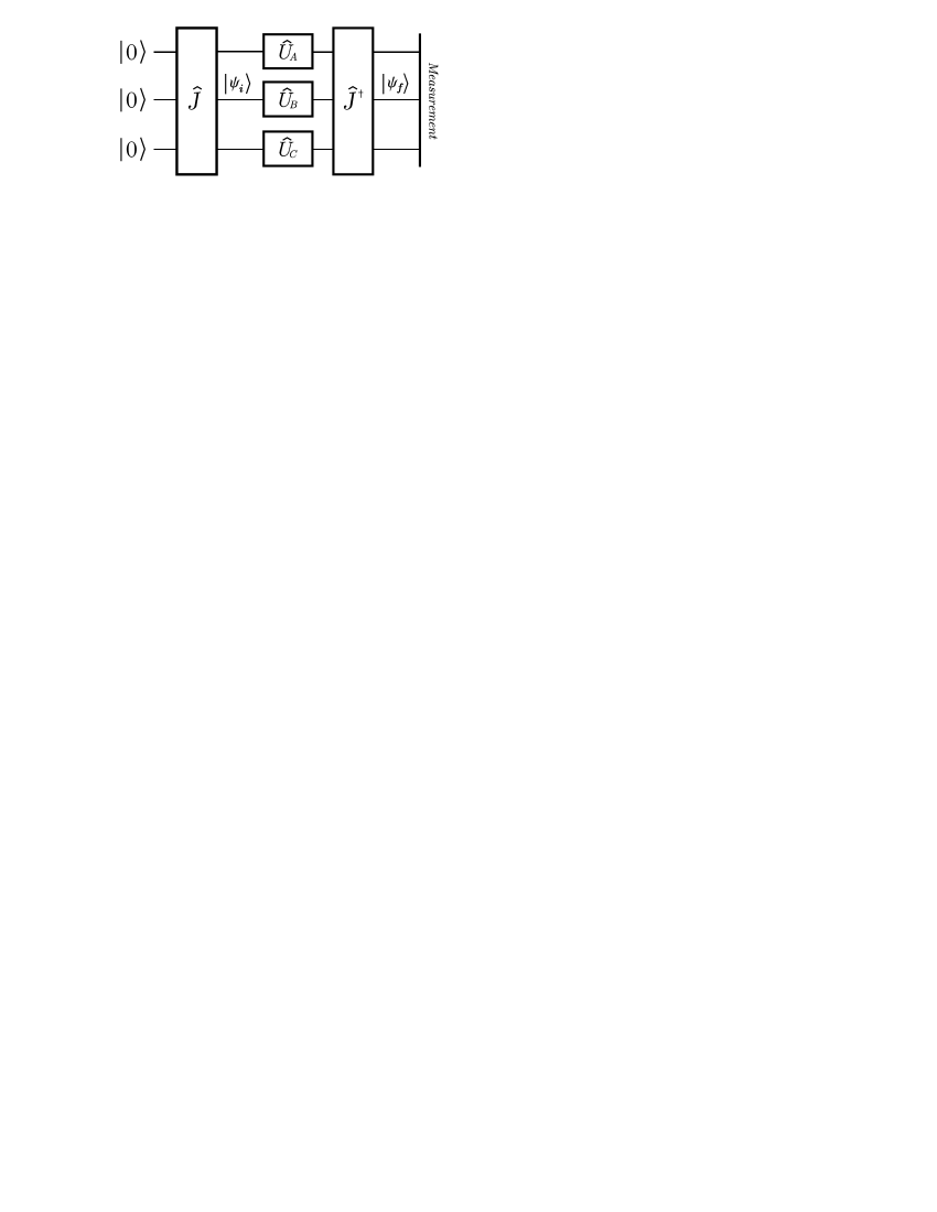
Figure 5: The setup of three-player quantum games.

2.2.3 Two-parameter strategic set

We start investigation of three-player Prisoner’s Dilemma with restricted strategic space, i.e. the strategic space is a two-parameter set[21]. The matrix representation of the corresponding operators is taken to be

$$\hat{U}\left(\theta,\varphi\right)=\left(\begin{array}[]{cc}\cos\theta/2&e^{i\varphi}\sin\theta/2\\ -e^{-i\varphi}\sin\theta/2&\cos\theta/2\end{array}\right)$$ (17)

with $0\leqslant\theta\leqslant\pi$ and $0\leqslant\varphi\leqslant\pi/2$. To be specific, $\hat{U}\left(0,0\right)$ is the identity operator $\hat{I}$ which corresponds to “Cooperate”, and $\hat{U}\left(\pi,\pi/2\right)=i\sigma_{x}$, which is equivalent to the bit-flipping operator, corresponds to “Defect”. Therefore $\hat{J}$ commutes with any operator formed from $i\sigma_{x}$ and $\hat{I}$ acting on different qubits, and this guarantees that the classical Prisoners’ Dilemma is faithfully entailed in the quantum game.

If there is no entanglement (for $\gamma=0$), the game is separable, i.e. at each instance the state of the game is separable. We find that any strategy profile formed from $\hat{U}\left(\pi,\pi/2\right)=i\sigma_{x}$ and $\hat{U}\left(\pi,0\right)=i\sigma_{y}$ is Nash equilibrium. However this property of multiple equilibria is a trivial one. For any profile of Nash equilibrium of the separable game, because $i\sigma_{x}\left|0\right\rangle=i\left|1\right\rangle$ and $i\sigma_{y}\left|0\right\rangle=-\left|1\right\rangle$, the final state $\left|\psi_{f}\right\rangle=-\left(-i\right)^{n}\left|1\right\rangle\left|1\right\rangle\left|1\right\rangle$, where $n$ denotes the number of players who adopts $\hat{U}\left(\pi/2,\pi\right)=i\sigma_{x}$. According to the payoff functions in Eq. (15), each player receives payoff $1$. Hence in this case $i\sigma_{x}$ and $i\sigma_{y}$ have the same effect to the payoffs. And in this sense, all the Nash Equilibria are equivalent to the classical strategy profile $(D,D,D)$. Indeed, the separable game does not exceed the classical game.

Although unentangled games is trivial, the behavior of maximally entangled game is fascinating and surprising. The profile $i\sigma_{x}\otimes i\sigma_{x}\otimes i\sigma_{x}$ is no longer the Nash equilibrium. However, a new Nash equilibrium, $i\sigma_{y}\otimes i\sigma_{y}\otimes i\sigma_{y}$ $\left(i\sigma_{y}=U(\pi,0)\right)$, emerges with payoffs

$$\$_{A}\left(i\sigma_{y},i\sigma_{y},i\sigma_{y}\right)=\$_{B}\left(i\sigma_{y},i\sigma_{y},i\sigma_{y}\right)=\$_{C}\left(i\sigma_{y},i\sigma_{y},i\sigma_{y}\right)=3.$$ (18)

Indeed, for $\gamma=\pi/2$,

$$\$_{A}\left(\hat{U}\left(\theta,\varphi\right),i\sigma_{y},i\sigma_{y}\right)=\left(2+2\cos 2\varphi\right)\sin^{2}\frac{\theta}{2}\leqslant 3=\$_{A}\left(i\sigma_{y},i\sigma_{y},i\sigma_{y}\right)$$ (19)

for all $\theta\in\left[0,\pi\right]$ and $\varphi\in\left[0,\pi/2\right]$. Analogously

$$\$_{B}\left(i\sigma_{y},\hat{U}\left(\theta,\varphi\right),i\sigma_{y}\right) \leqslant \$_{B}\left(i\sigma_{y},i\sigma_{y},i\sigma_{y}\right),$$

$$\$_{C}\left(i\sigma_{y},i\sigma_{y},\hat{U}\left(\theta,\varphi\right)\right) \leqslant \$_{C}\left(i\sigma_{y},i\sigma_{y},i\sigma_{y}\right).$$ (20)

Hence, no player can improve his individual payoff by unilaterally deviating from the strategy $i\sigma_{y}$, i.e. $\left(i\sigma_{y},i\sigma_{y},i\sigma_{y}\right)$ is a Nash equilibrium. It is interesting to see that the payoffs for the players are $\$_{A}=\$_{B}=\$_{C}=3$, which are the best payoffs that retain the symmetry of the game. Thus the strategy profile $(i\sigma_{y},i\sigma_{y},i\sigma_{y})$ has the property of Pareto Optimal, i.e. no player can increase his payoff without lessening the payoff of the other players by deviating from this pair of strategies. Therefore by allowing the players to adopt quantum strategies, the dilemma that exists in the classical game is completely removed when the game is maximally entangled.

In the above paragraph, we have considered the maximally entangled game. In this case, an novel Nash equilibrium $\left(i\sigma_{y},i\sigma_{y},i\sigma_{y}\right)$ emerges, which has the property of Pareto optimal. Since the key role of entanglement in quantum information, it will be interesting to investigate whether this strategy profile is still Nash equilibrium when the game is not maximal entangled. And if it is, how the property of the game changes with the variations of the entanglement when the players each resort to $i\sigma_{y}=U(\pi,0)$. The surprising thing is that $i\sigma_{y}\otimes i\sigma_{y}\otimes i\sigma_{y}$ is always a Nash equilibrium for any $\gamma\in\left(0,\pi/2\right)$. The proof that this pair of strategy is still Nash equilibrium runs as follows. Assume Bob and Colin adopt $i\sigma_{y}$ as their strategies, the payoff function of Alice respect to her strategy $\hat{U}\left(\theta,\varphi\right)$ is

$$\$_{A}\left(\hat{U}\left(\theta,\varphi\right),i\sigma_{y},i\sigma_{y}\right) = \left(1+2\cos^{2}\varphi\sin^{2}\gamma\right)\sin^{2}\frac{\theta}{2}$$ (21)

$$\leqslant 1+2\sin^{2}\gamma=\$_{A}\left(i\sigma_{y},i\sigma_{y},i\sigma_{y}\right).$$

So, $i\sigma_{y}$ is her best reply to the other players. Since the game is symmetric, the same holds for Bob and Colin. Therefore, no matter what the amount of the game’s entanglement is, $i\sigma_{y}\otimes i\sigma_{y}\otimes i\sigma_{y}$ is always a Nash equilibrium for the game. It is fascinating to see that the payoff of the players is a monotonously increasing function of amount of the entanglement,

$$\$_{A}\left(i\sigma_{y},i\sigma_{y},i\sigma_{y}\right)=\$_{B}\left(i\sigma_{y},i\sigma_{y},i\sigma_{y}\right)=\$_{C}\left(i\sigma_{y},i\sigma_{y},i\sigma_{y}\right)=1+2\sin^{2}\gamma.$$ (22)

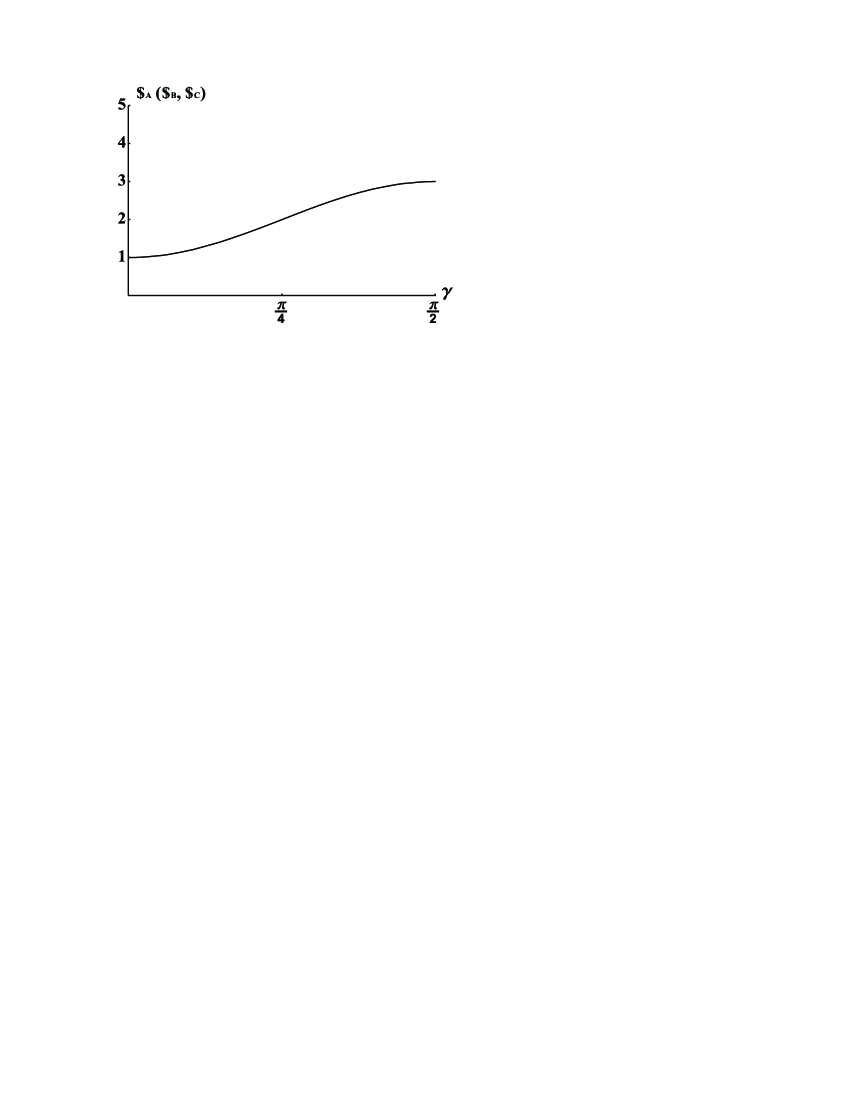
Figure 6: The payoff plot as a function of $\gamma$ when all the players resort to Nash Equilibrium, $i\sigma_{y}\otimes i\sigma_{y}\otimes i\sigma_{y}$. From this figure we can see that the payoffs of the players are the same and are monotonous increasing function of $\gamma$.

Fig 6 illustrates how the payoffs depend on the amount of entanglement when the players all resort to Nash equilibrium. From this figure, we can see that entanglement dominates the property of the game: the payoffs of the players are the same, which is a monotonous increasing function of the amount of entanglement of the game’s initial state. The profile $i\sigma_{y}\otimes i\sigma_{y}\otimes i\sigma_{y}$ is always a Nash equilibrium of the game independent of the entanglement, and the dilemma is completely removed when the measure of game’s entanglement $\gamma$ increases to its maximum $\pi/2$.

2.2.4 General unitary operations

In this section, we turn our attention to a more general situation, in which players are allowed to adopt strategies from the whole unitary operations. Just like in the two-player situation, the unitary operation can be denoted as in Eq. (9). Therefore a player’s strategy can be represented by a vector $\left(w,x,y,z\right)$.

At first, let us consider the case when the amount of entanglement is maximal. We have known that in two player’s Prisoner’s Dilemma, there is no pure strategy Nash equilibrium existing of the whole unitary space. However, the situation is completely different in the three-player version of this game. There indeed exist six symmetric Nash Equilibria strategy profiles $K_{1}\otimes K_{1}\otimes K_{1}$, $\cdots\cdots$, $K_{6}\otimes K_{6}\otimes K_{6}$ with

$$K_{1} = \left(\frac{1}{\sqrt{2}},0,\frac{1}{\sqrt{2}},0\right),$$

$$K_{2} = \left(\frac{1}{\sqrt{2}},0,-\frac{1}{\sqrt{2}},0\right),$$

$$K_{3} = \left(-\frac{1}{2\sqrt{2}},\frac{\sqrt{3}}{2\sqrt{2}},\frac{1}{2\sqrt{2}},\frac{\sqrt{3}}{2\sqrt{2}}\right),$$

$$K_{4} = \left(\frac{1}{2\sqrt{2}},-\frac{\sqrt{3}}{2\sqrt{2}},\frac{1}{2\sqrt{2}},\frac{\sqrt{3}}{2\sqrt{2}}\right),$$

$$K_{5} = \left(\frac{1}{2\sqrt{2}},\frac{\sqrt{3}}{2\sqrt{2}},-\frac{1}{2\sqrt{2}},\frac{\sqrt{3}}{2\sqrt{2}}\right),$$

$$K_{6} = \left(\frac{1}{2\sqrt{2}},\frac{\sqrt{3}}{2\sqrt{2}},\frac{1}{2\sqrt{2}},-\frac{\sqrt{3}}{2\sqrt{2}}\right).$$

These six Nash Equilibria are symmetric to the players and yields the same payoff $11/4$ to the three players. Hence, these Nash equilibrium keeps the symmetry and fairness of the game, and are more efficient than the classical Nash equilibrium $(D,D,D)$. In the following, we will take $K_{1}\otimes K_{1}\otimes K_{1}$ as an example to prove that it is truly a Nash equilibrium of the game. We write the strategy $K_{1}$ in matrix form

$$K_{1} = \frac{1}{\sqrt{2}}\cdot I+0\cdot i\sigma_{x}+\frac{1}{\sqrt{2}}\cdot i\sigma_{y}+0\cdot i\sigma_{z}$$

$$= \left(\begin{array}[]{cc}\frac{1}{\sqrt{2}}&\frac{1}{\sqrt{2}}\\ -\frac{1}{\sqrt{2}}&\frac{1}{\sqrt{2}}\end{array}\right).$$

Assume Bob and Colin both choose strategy $K_{1}$, according to payoff function of Alice (see Eq. (15))

$$\$_{A}(U_{A},K_{1},K_{1})=\frac{1}{4}\left[11\left(w^{2}+y^{2}\right)+10\left(x^{2}+z^{2}\right)\right].$$ (24)

From Eq. (24), we can see that $\$_{A}(U_{A},K_{1},K_{1})$ reaches maximum if $w^{2}+y^{2}=1$. It is obviously that $w=y=1/\sqrt{2}$ satisfies this condition. Therefore, Alice can get her best payoff when she chooses $K_{1}$ against the other two players’ strategies $K_{1}\otimes K_{1}$. Because the game is symmetric, the same analysis is true for Bob and Colin. So $K_{1}\otimes K_{1}\otimes K_{1}$ is a Nash equilibrium of the game for the whole set of unitary operations, which means that no player can increase his individual payoff by unilateral deviating from the strategy profile. From our proof, we can see that when both Bob and Colin adopt $K_{1}$, there exist other strategies that can yield the maximal payoff $11/4$ to Alice. Hence, $K_{1}\otimes K_{1}\otimes K_{1}$ is Nash equilibrium, but not a strict one, as are the other five equilibria.

2.2.5 Non-maximal entanglement situation

Unlike the situation of restricted strategic space, this time the non-maximal entanglement situation is more complex and more interesting. Since the solution we study here is symmetric and fair to the players, we will take Alice as an instance.

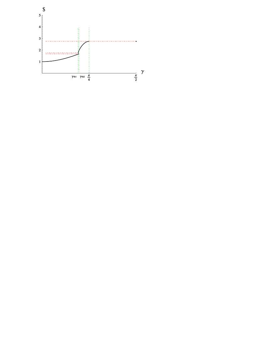
Figure 7: The expected payoff for Alice as a function of the measure of the parameter $\gamma$ when all players resort to Nash Equilibrium strategies.

Fig 7 depict Alice Payoff as a function of $\gamma$ when the players all resort to Nash equilibrium strategy. From Fig 7, we see that the entanglement of the game is divided into four domain by three thresholds, that are

$$\gamma_{th1} = \arccos\sqrt{\frac{1}{26}\left(13+\sqrt{\frac{3}{221}\left(759+128\sqrt{42}\right)}\right)}\cong 0.60276,$$

$$\gamma_{th2} = \arcsin\sqrt{\frac{1}{3}}\cong 0.61548,$$

$$\gamma_{th3} = \frac{\pi}{4}\cong 0.78539.$$ (25)

In the domain $0\leqslant\gamma\leqslant\gamma_{th2}$, there exist four Nash equilibria of the game, which are $\left(0,0,\pm 1,0\right)$ and $\left(0,\frac{\sqrt{3}}{2},\pm\frac{1}{2},0\right)$. These four Nash equilibria yield the same payoff $1+2\sin^{2}\gamma$. Hence, the player’s reward is a monotonous increasing function of $\gamma$, i.e. the game’s property is enhance by the property of the game’s entanglement. In the domain $\gamma_{th1}\leqslant\gamma\leqslant\gamma_{th3}$, the situation is very complex. The Nash equilibria of the game can be represented as the following:

$$\pm\left[a\left(\gamma\right)\left(0,0,1,0\right)-b\left(\gamma\right)\left(0,0,0,\pm 1\right)\right]$$

and

$$\pm\left[a\left(\gamma\right)\left(\frac{\sqrt{3}}{2},0,0,\pm\frac{1}{2}\right)-b\left(\gamma\right)\left(0,\frac{\sqrt{3}}{2},\pm\frac{1}{2},0\right)\right],$$

where $a\left(\gamma\right)$, $b\left(\gamma\right)>0$ and $a\left(\gamma\right)^{2}+b\left(\gamma\right)^{2}=1$. From Fig 7, we see that (i) the payoff in this domain is bigger than the first domain and (ii) it also increases with the increasing of entanglement. Hence, we can also get the conclusion that in this domain, the game’s property can be enhanced by the entanglement of the game’s state. In the domain $\gamma_{th3}\leqslant\gamma<\pi/2$, there is no symmetric pure Nash equilibrium. This situation is the same as the two-player version of this game.

3 Conclusion

In this paper, we present the systematic investigation of quantum games with the particular case of the Prisoner’s Dilemma. By considering different situations, the game shows properties which may outperform the classical version of this game.

Quantum games and quantum strategies is a burgeoning field of quantum information and quantum computation theory. Assuming the players are playing the game by quantum rules, the game’s solution is more efficient than the classical one. Such quantum games are not just esoteric exercises. They could form part of the longed-for quantum technologies of tomorrow, such as ultra-fast quantum computers. They might even help traders construct a crash-resistant stock market. And quantum games could provide new insights into puzzling natural phenomena such as high-temperature superconductivity etc.. Although at this stage, no one is sure which applications will prove most fruitful, it is sure that quantum game theory is a potential and promising research field[3]. Playing by quantum rules, every one will become a winner[22].

References

- [1] O. Morgenstern and J. von Neumann, Theory of Games and Economic Behavior, Princeton University Press, Princeton (1944).
- [2] M. A. Nowak and K. Sigmund, Phage-lift for game theory, Nature 398 (1999) 367–368.
- [3] E. Klarreich, Playing by quantum rules, Nature 414 (2001) 244–245.
- [4] D. A. Meyer, Quantum Strategies, Phys. Rev. Lett. 82 (1999) 1052–1055.
- [5] D. A. Meyer, Quantum games and quantum algorithms, LANL preprint, quant-ph/0004092.
- [6] J. Eisert, M. Wilkens and M. Lewenstein, Quantum Games and Quantum Strategies, Phys. Rev. Lett. 83 (1999) 3077–3080.
- [7] J. Du, X. Xu, H. Li, X. Zhou and R. Han, Entanglement playing a dominating role in quantum games, Phys. Lett. A 289 (2001) 9–15.
- [8] L. Marinatto and T. Weber. A quantum approach to static games of complete information, Phys. Lett. A 272 (2000) 291–303.
- [9] A. Iqbal and A. Toor, Evolutionarily stable strategies in quantum games, Phys. Lett. A 280 (2001) 249–256.
- [10] J. Du, H. Li, X. Xu, M. Shi, J. Wu, X. Zhou and R. Han, Experimental Realization of Quantum Games on a Quantum Computer, Phys. Rev. Lett, 88 (2002) 137902(1–4).
- [11] N. F. Johnson, Playing a quantum game with a corrupted source, Phys. Rev. A 63 (2001) 020302(1-4).
- [12] S. C. Benjamin and P. M. Hayden, Multiplayer quantum games, Phys. Rev. A 64 (2001) 030301(1-4).
- [13] A. P. Flitney, J. Ng and D. Abbott, Quantum Parrondo’s Games, Physica A 314 (2002) 384–391.
- [14] G. M. D’Ariano, R. D. Gill, M. Keyl, B. Kuemmerer, H. Maassen, R. F. Werner, The Quantum Monty Hall Problem, Quant. Inf. Comput. 2, No. 5, 355–366 (2002).
- [15] P. Ball, Physicists play by quantum rules, Nature Science Update, 03 Apr. 2002.
- [16] F. Morikoshi, Recovery of Entanglement Lost in Entanglement Manipulation, Phys. Rev. Lett. 84 (2000) 3189–3192.
- [17] J. Eisert and M. Wilkens, Catalysis of Entanglement Manipulation for Mixed States, Phys. Rev. Lett. 85 (2000) 437–440.
- [18] S. C. Benjamin and P. M. Hayden, Comment on ”Quantum Games and Quantum Strategies”, Phys. Rev. Lett. 87 (2001), 069801.
- [19] J. Eisert and M. Wilkens, Quantum Games, J. Mod. Opt. 47 (2000) 2543–2556.
- [20] J. Du, H. Li, X. Xu, X. Zhou and R. Han, Phase Transitions in Quantum Games, quant-ph/0111138.
- [21] J. Du, H. Li, X. Xu, X. Zhou and R. Han, Entanglement enhanced multiplayer quantum games, Phys. Lett. A, 302 (2002) 229–233.
- [22] P. Ball, Everyone wins in quantum games, Nature Science Update, 18 Oct. 1999.