Transmission through a potential barrier in quantum mechanics of multiple degrees of freedom: complex way to the top.

Abstract

A semiclassical method for the calculation of tunneling exponent in systems with many degrees of freedom is developed. We find that corresponding classical solution as function of energy form several branches joint by bifurcation points. A regularization technique is proposed, which enables one to choose physically relevant branches of solutions everywhere in the classically forbidden region and also in the allowed region. At relatively high energy the physical branch describes tunneling via creation of a classical state, close to the top of the barrier. The method is checked against exact solutions of the Schrödinger equation in a quantum mechanical system of two degrees of freedom.

I Introduction

Semiclassical methods provide a very useful tool for the study of nonperturbative processes. Tunneling phenomena represent one of the most notable cases where semiclassical techniques can be used to obtain otherwise unattainable information on transition probabilities. There are many cases where the application of semiclassical methods reduces to having to solve the classical equations of motion in the Euclidean time domain, namely with $t$ analytically continued to $i\tau$. A famous example is WKB approximation to tunneling in quantum mechanics with one degree of freedom. In systems with multiple degrees of freedom there are other, more complex situations, however, where the evolution along the imaginary time axis cannot be treated separately from the real time evolution which precedes and follows it. This happens, for example, in the study of tunneling in high-energy collisions in field theory Kuznetsov:1997az ; Bezrukov:2001dg , where one must consider a system with definite particle number in the initial state, or in the study of chemical reactions where the initial system is in a definite quantum state Miller . Then, in the search for complex-time solutions of the classical equations of motion that dominate tunneling, one encounters a novel phenomenon which, if not properly handled, may make it impossible to obtain the appropriate solutions. We ran into this kind of problems in the study of an interesting class of field theoretical processes, where tunneling occurs between different topological sectors and is accompanied by baryon number violation 'tHooft:1976fv ; Ringwald:1990ee ; Espinosa:1990qn ; Bezrukov:2001dg . However, the specifics of the model are immaterial for the features of tunneling which we plan to describe in this paper. Indeed, the fact that, with a field theoretical system, one is dealing with an infinite number of degrees of freedom is also irrelevant for the appearance of the phenomenon that we alluded to above: this phenomenon emerges as soon as one deals with more than one degree of freedom and in quite a range of applications of semiclassical techniques. For this reason we decided to illustrate it in this paper in the context of a simple quantum mechanical system with two degrees of freedom. The problems one encounters in the study of the field theoretical system and their solution will be described in a separate paper BLRRT:prepare . Our hope is that the discussion presented here may help to shed some light on how semiclassical methods can be effectively applied in situations which a priory may seem intractable.

Our considerations are of quite general validity, but, for purposes of clarity, it is useful to present them in the context of a definite model. We will take this to be the model of Ref. Bonini:1999kj ; Bonini:1999cn , namely a system formed by two particles of identical mass $m$, moving in one dimension and bound by a harmonic oscillator potential of frequency $\omega$ (Fig. 1).

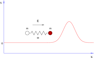
Figure 1: Oscillator hitting a potential barrier, with which only the “dark” particle interacts.

One of the particles interacts with a repulsive potential barrier. This potential barrier is assumed to be high and wide, while the spacing between the oscillator levels is much smaller than the barrier height $V_{0}$. Thus, the Hamiltonian of the model is

$$H=\frac{p_{1}^{2}}{2m}+\frac{p_{2}^{2}}{2m}+\frac{m\omega^{2}}{4}(x_{1}-x_{2})^{2}+V_{0}\mathrm{e}^{-x_{1}^{2}/2\sigma^{2}}\;,$$ (1)

where the conditions on the oscillator frequency and potential barrier are

$$\hbar\omega\ll V_{0},$$ (2)

$$\sigma\gg\hbar/\sqrt{mV_{0}}\;.$$

The problem is to calculate the transition probability through the barrier for a given incoming bound state; since the variables do not separate, this is certainly a non-trivial problem. Quantum-mechanically the incoming state is fully characterized by its total energy $E$ and oscillator excitation number $N$. For $E<V_{0}$ the transition through the barrier can happen only through tunneling. However, the transition may be classically forbidden, and occur through tunneling, also if $E>V_{0}$. A detailed study of the model (Ref. Bonini:1999kj ; Bonini:1999cn ) shows that one can distinguish two regions in the $E-N$ plane, as illustrated in Fig. 2: region A where transition across the barrier is classically forbidden, and region B where it is classically allowed. (Since $\hbar\omega(N-\frac{1}{2})$ cannot exceed $E$, the further region with $N>E/\hbar\omega-\frac{1}{2}\simeq E/\hbar\omega$ is trivially excluded.) The vertex S of B marks the lowest energy at which one can have a classically allowed transition, characterized by $E=E_{S}=V_{0}$ and some definite initial excitation number $N=N_{S}$. Strictly speaking, in order to have a classically allowed transition the energy must be (infinitesimally) larger than $E_{S}$. For $E=E_{S}$ there exists a static, unstable solution to the classical equations of motion, where the system just sits on top of the barrier: $x_{1}=x_{2}=0$. In the study of field theoretical tunneling processes this solution has been called the sphaleron Klinkhamer:1984di and, for sake of terminology, we will use the term also in this article, but no special meaning should be attributed here to it: for us it will be just a name. The line $E_{\mathrm{PI}}$ in Fig. 2 marks a special class of tunneling solutions to the equations of motion, about which more will be said later.

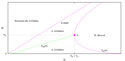
Figure 2: Allowed and forbidden regions in the model with two degrees of freedom.

In the region A one would like to calculate the exponent $F(E,N)$ in the transition probability $\mathcal{T}\approx\exp(-F/\hbar)$. The boundary between regions A and B is given by the line $E_{0}(N)$, where $F(E,N)=0$. $F$ can be calculated by the method introduced in Ref. Rubakov:1992ec , which will be recapitulated later. (See also the earlier work by Miller Miller for an elegant approach to the calculation of the transition probability, based on canonical transformations.) The method of Ref. Rubakov:1992ec leads to having to solve the classical equations of motion, after analytic continuation to complex time and complex phase space, subject to suitable boundary conditions. In the tunneling solutions, the system evolves along the real time direction first, then undergoes the under-barrier evolution along the imaginary time direction. For the solutions situated on the line $E_{\mathrm{PI}}$ in Fig. 2, the coordinates of the particles are real throughout the evolution, but this is a very special case. For general tunneling solutions the coordinates and the corresponding momenta, have to be continued to complex values. This is a defining feature of processes with more than one degree of freedom: in systems where a single particle moves along a line and tunnels under a potential barrier, all tunneling solutions would be real and behave like the processes on the line $E_{\mathrm{PI}}$. In systems with multiple degrees of freedom tunneling solutions, i.e. evolutions which obey the classical (analytically continued) equations of motion and obey the appropriate boundary conditions, can be rather readily found for $E<E_{S}$. As the energy approaches the barrier height, however, something special happens: in the tunneling solutions the system lingers for progressively longer times on top of the barrier and the boundary conditions become truly asymptotic in time. Rigorously, finite time evolutions that satisfy the boundary conditions cease to exist. Here lies the subtlety in the application of semiclassical methods to such processes and the root of the difficulty in finding solutions that can be used throughout the domain of classically forbidden transitions (i.e. the whole of region A). As we plan to show in this paper, the difficulty can be overcome by employing a suitable regularization, and one can find physically relevant solutions which map the entire region of classically forbidden processes and also merge continuously with classically allowed evolutions as one approaches the boundary $E_{0}(N)$. The new solutions we find all describe tunneling onto the top of the potential barrier, or onto long-living excitations above the top. Notice that the problem is special to transitions which have an energy larger than the barrier height (i.e. larger than the sphaleron energy) and thus would never be encountered in systems with a single degree of freedom, the systems normally used in textbooks to illustrate the use of semiclassical techniques, where all processes with energy larger than the barrier height are classically allowed. Still, even in simple systems with a single degree of freedom, one can see a sign of the subtleties that one can, and does encounter in more complex systems. For this reason, and also in order to put our whole formulation on a clear footing, we will start by re-examining the semiclassical description of tunneling in the case of a single particle moving on a line. This will be done in Sec. II.

In Sec. III we consider the quantum mechanical model with two degrees of freedom. In particular, in Sec. III.1 we introduce the semiclassical technique for the calculation of the tunneling exponent. Then we examine the classical over-barrier solutions and find the boundary of the classically allowed region $E_{0}(N)$ in Sec. III.2. In Sec. III.3 we present a straightforward application of the semiclassical technique, outlined in Sec. III.1, and find that it ceases to produce the relevant classical solutions in a part of the tunneling region A, roughly speaking, at $E>E_{\mathrm{S}}$. In Sec. IV we introduce our regularization technique and show that it indeed enables one to find the tunneling classical solutions in the entire region A (Sec. IV.1). We check our method against the numerical solution of the full Schrödinger equation in Sec. IV.2. In Sec. IV.3 we show how our regularization technique may be used to join smoothly the classically allowed and classically forbidden regions. Our conclusions are presented in Sec. V.

II Quantum mechanics of one degree of freedom

II.1 Classical boundary value problem

Let us review the derivation of the semiclassical expression for the tunneling exponent in quantum mechanics of one degree of freedom. The result is well known in this case (WKB formula) and the derivation here may seem artificially complicated, but it can be generalized to the case of multiple degrees of freedom, while many of its general features can still be captured in the relatively simple case of one degree of freedom.

Let us calculate the probability of tunneling through a potential barrier, located in a region near $X=0$, from the asymptotic region $X\to-\infty$. Let us use a system of units with $\hbar=1$ and set the mass of a particle equal to 1 (both can be reintroduced in our formulas on dimensional grounds). The Hamiltonian we consider has the general form

$$\hat{H}=\left(\frac{\hat{P}^{2}}{2}+V(\hat{X})\right)\;,$$ (3)

where the potential $V(X)$ has the form

$$V(X)=\frac{1}{\lambda}U(\sqrt{\lambda}X)$$

and rapidly decays as $X\to\pm\infty$. Then the semiclassical limit of this model is obtained when $\lambda\to 0$ while the energy is kept parametrically large: $E=\tilde{E}/\lambda$.

The probability of tunneling from an incoming ($X\to-\infty$) state with energy $E$ is

$$\mathcal{T}(E)=\lim_{t_{f}-t_{i}\to\infty}\int\limits_{0}^{+\infty}dX_{f}\left|\langle X_{f}|\mathrm{e}^{-i\hat{H}(t_{f}-t_{i})}|E\rangle\right|^{2}\;,$$ (4)

where it is implicit that the initial state $|E\rangle$ is a wave packet with very small spread in momentum $P$, centered at large negative $X$. The transition amplitude

$$\mathcal{A}_{fi}=\langle X_{f}|\mathrm{e}^{-i\hat{H}(t_{f}-t_{i})}|X_{i}\rangle$$

and its complex conjugate $\mathcal{A}_{i^{\prime}f}^{*}$ have the standard path integral representation

$$\mathcal{A}_{fi} = \int[dX]\Bigg{|}_{\stackrel{{\scriptstyle\scriptscriptstyle X(t_{i})=X_{i}}}{{\scriptscriptstyle X(t_{f})=X_{f}}}}\mathrm{e}^{iS[X]}\;,$$ (5)

$$\mathcal{A}_{i^{\prime}f}^{*} = \int[dX^{\prime}]\Bigg{|}_{\stackrel{{\scriptstyle\scriptscriptstyle{X}^{\prime}(t_{i})=X^{\prime}_{i}}}{{\scriptscriptstyle{X}^{\prime}(t_{f})=X_{f}}}}\mathrm{e}^{-iS[X^{\prime}]}\;,$$

where $S[X]=\int_{t_{i}}^{t_{f}}L(X,\dot{X})dt$ is the action of the model. Inserting factors $\int dX_{i}\;|X_{i}\rangle\langle X_{i}|=1$ one re-expresses (4) in terms of these transition amplitudes and the initial state matrix elements

$${\cal B}_{ii^{\prime}}=\langle X_{i}|E\rangle\langle E|X_{i}^{\prime}\rangle$$

in the following way,

$$\mathcal{T}(E)=\lim\limits_{t_{f}-t_{i}\to\infty}\int\limits_{0}^{+\infty}dX_{f}\int\limits_{-\infty}^{0}d{X}_{i}d{X}_{i}^{\prime}\,\mathcal{A}_{fi}\mathcal{A}_{i^{\prime}f}^{*}\mathcal{B}_{ii^{\prime}}.$$ (6)

To obtain an integral representation of the initial-state matrix elements, let us rewrite ${\cal B}_{ii^{\prime}}$ as follows,

$${\cal B}_{ii^{\prime}}=\langle X_{i}|\hat{P}_{E}|X_{i}^{\prime}\rangle\;,$$ (7)

where $\hat{P}_{E}$ denotes the projector onto a state with total energy $E$. In the momentum basis this projector has an integral representation which follows from the integral representation of the $\delta$–function:

$$\langle Q|\hat{P}_{E}|P\rangle=\frac{\sqrt{2E}}{2\pi}\int\!d\xi\,\mathrm{e}^{-i(E-\frac{P^{2}}{2})\xi}\,\delta(Q-P)\;,$$ (8)

where $|Q\rangle$, $|P\rangle$ are the momentum eigenstates. It is convenient to introduce the notation

$$T=-i\xi\;.$$

Combining formulas (5), (6), (7), (8), and evaluating the Gaussian integrals over $P$ and $Q$, one obtains the path integral representation for the tunneling probability. After rescaling $X\to X/\sqrt{\lambda},\;X^{\prime}\to X^{\prime}/\sqrt{\lambda}$ it takes the following form

$$\mathcal{T}(E)=\lim\limits_{t_{f}-t_{i}\to\infty}\Bigg{\{}\int\limits_{-i\infty}^{+i\infty}dT\int[dX\,dX^{\prime}]\\ \exp\left[-\frac{1}{\lambda}F[X,X^{\prime};T]\right]\Bigg{\}},$$ (9)

where the integration over $X_{i}$, $X^{\prime}_{i}$ and $X_{f}$ is implicit, and

$$F[X,X^{\prime};T]=-iS[X]+iS[X^{\prime}]\\ -\tilde{E}T+\frac{(X_{i}-X_{i}^{\prime})^{2}}{2T}\;,$$ (10)

with $\tilde{E}=\lambda E$ being the rescaled energy (independent of $\lambda$ in the semiclassical limit $\lambda\to 0$). In this paper we will omit the tilde over the rescaled parameters, where this does not cause confusion.

At small $\lambda$ one applies the saddle point approximation to the integral (9). We will not consider the pre-exponential factor in the probability, so we will be interested in the saddle point value of $F$. The saddle point equations for $X(t)$ and $X^{\prime}(t)$ are the classical equations of motion,

$$\frac{\delta S(X)}{\delta X}=0\;,\quad\frac{\delta S(X^{\prime})}{\delta X^{\prime}}=0\;,$$ (11)

while the variation with respect to the boundary values $X_{f}$, $X_{i}$, $X^{\prime}_{i}$ and auxiliary variable $T$ leads to the boundary conditions

$$P_{f}=P^{\prime}_{f}\;,$$ (12a)

$$P_{i}=P^{\prime}_{i}=-\frac{X_{i}-X^{\prime}_{i}}{iT}\;,$$ (12b)

$$E=-\frac{(X_{i}-X^{\prime}_{i})^{2}}{2T^{2}}\;,$$ (12c)

where $$P\equiv\dot{X}$$. Note also, that one has (see Eq. (5))

$$X(t_{f})=X^{\prime}(t_{f})=X_{f}\;,$$ (12d)

and that Eq. (12c) may be written in the form $E=P_{i}^{2}/2$. The latter equation requires that the energy of the solution is equal to $E$. One more observation is that

$$X^{\prime}=X^{*}\;,$$ (13)

because $X^{\prime}$ corresponds to the saddle point of the complex conjugate amplitude. Equations (12a) and (12d) simply mean that the solutions $X(t)$ and $X^{\prime}(t)$ coincide as $t\to+\infty$. On the other hand, Eq. (12b) states that the solutions $X(t)$ and $X^{\prime}(t)$ are different at initial time $t\to-\infty$, if the saddle point value of $T$ is not zero. There is no contradiction: for energy $E$ larger than the barrier height, a real classical trajectory running from $X\to-\infty$ to $X\to+\infty$ exists; for this solution $T=0$ and $X$ coincides with $X^{\prime}$ at any moment of time. On the other hand, if $E$ is smaller than the barrier height, then there is no such classical solution in real time, but the solution may exist on a contour in the complex time plane, which wraps around some branch point (as shown in Fig. 3). The solution continued along this contour is in general complex at large negative times (region A’ in Fig. 3). Then equations (12b), (12c) and (13) guarantee that the saddle point value of $T$ is real.

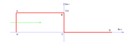
Figure 3: Contour in the complex time plane.

The boundary conditions may be significantly simplified by shifting the initial time from the real axis. As $\mathop{\mathrm{Re}}t\to-\infty$, the potential is irrelevant, and any solution describes free motion with momentum $P_{i}=\sqrt{2E}$,

$$X(t)=X_{i}+P(t-t_{i})\;,$$

$$X^{\prime}(t)=[X(t)]^{*}\;.$$

Let us choose the initial time in such a way that $\mathop{\mathrm{Im}}t=T/2$, i.e. consider the boundary value problem (11), (12) on the contour ABCD of Fig. 3. Then Eq. (12b) takes a simple form

$$\frac{X^{*}(t)-X(t)}{iT}=0\,,$$

$$t=t^{\prime}+\frac{iT}{2}\,,\quad t^{\prime}=\text{real}\to-\infty\;,$$

which simply means that the coordinate is real on the part AB of the time contour. Equation (13) implies that the solution is real in the asymptotic region D, i.e. at $t=\text{real}\to+\infty$. Hence, instead of Eq. (12d) one has reality conditions in the asymptotics A and D. After obtaining the solution to the classical boundary value problem, one inserts it to the right hand side of Eq. (10) and obtains

$$F(E)=2\mathop{\mathrm{Im}}S-ET\;,$$ (14)

where $S$ is the classical action on the contour ABCD.

In quantum mechanics of one degree of freedom, the contour ABCD may be chosen in such a way that the points B and C are the turning points of the solution. Then the solution is real also at the part BC of the contour. Indeed, a real solution at the part BC of the contour oscillates in the upside-down potential, $T/2$ equals to half-period of oscillations, and the points B and C are the two different turning points, $\dot{X}=0$ (see Fig. 4).

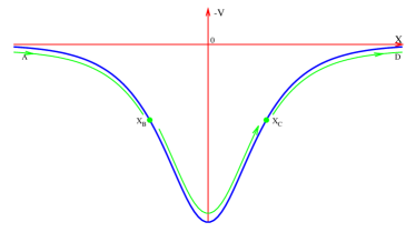
Figure 4: Classical solution describing tunneling.

The continuation of this solution, according to the equation of motion, from the point C to the positive real times corresponds to the real-time motion, from the point $X_{C}$ with zero initial velocity, towards $X\to+\infty$; the coordinate $X(t)$ stays real on the part CD of the contour. Likewise, the continuation back in time from the point C leads to real solution in the part AB of the contour. In this way the reality conditions are satisfied at A and D. The only contribution to $F$ comes from the Euclidean part of the contour, and one can check that the expression (14) reduces to

$$F(E)=2\int\limits_{X_{B}}^{X_{C}}\!\sqrt{2(V(X)-E)}\,dX\;,$$ (15)

which is the standard WKB result.

To summarize, in quantum mechanics of one degree of freedom, the semiclassical calculation of the tunneling exponent may be performed by solving the classical equation of motion on the contour ABCD in complex time plane, with the conditions that the solution be real in the asymptotic past (region A), and asymptotic future (region D). The relevant solutions tend to $X\to-\infty$ and $X\to+\infty$ in regions A and D, respectively. The auxiliary parameter $T$ is related to the energy of incoming state by the requirement that the energy of the classical solution equals to $E$. The exponent for the transition probability is given by Eq. (14), which, in fact, coincides with the WKB result (15).

II.2 Joining the allowed and forbidden regions

The solutions appropriate in the classically forbidden and classically allowed regions apparently belong to quite different branches. It is clear from Fig. 4 that as the energy approaches the height of the barrier $V_{0}$ from below, the amplitude of the oscillations in the upside-down potential decreases, while the period $T$ tends to a finite value determined by the curvature of the potential at its maximum. On the other hand, the solutions for $E>V_{0}$ (classically allowed region) always run along the real time axis, so the parameter $T$ is always zero. Hence, the relevant solutions do not merge at $E=V_{0}$, and $T(E)$ has a discontinuity at $E=V_{0}$. We find it instructive to develop a regularization technique that removes this discontinuity and allows for smooth transition through the point $E=V_{0}$. The reason is that in quantum mechanics of multiple degrees of freedom, similar points exist not only at the boundary of the classically allowed region, but also well inside the forbidden region (but still at $E>E_{S}$, see Introduction and Sec. III.2).

To illustrate the situation, let us consider an exactly solvable model with

$$U(X)=\frac{1}{\cosh^{2}X}\;.$$

The solution of the classical boundary value problem for energy smaller than the barrier height, $E<V_{0}\equiv 1$, is

$$\sqrt{\frac{E}{1-E}}\;\sinh X=-\cosh\left(\sqrt{2E}(t-t_{0})\right)\;.$$ (16)

This solution has branch points at $t^{\pm}_{*}$, where the potential becomes singular ($\cosh X=0$):

$$t^{\pm}_{*}-t_{0}=\frac{1}{\sqrt{2E}}\left(\pm\log\frac{1+\sqrt{E}}{\sqrt{1-E}}+i\frac{\pi}{2}+i\pi n\right)\;.$$ (17)

The requirement that the solution is real on the part AB of the contour determines the imaginary part of $t_{0}$,

$$\mathop{\mathrm{Im}}t_{0}=T/2\;.$$ (18)

To fix the translational invariance along real time, one imposes a constraint on $\mathop{\mathrm{Re}}t_{0}$. The solutions that are real at imaginary (Euclidean) time are obtained for

$$\mathop{\mathrm{Re}}t_{0}=0\;.$$

Later on, another choice will be convenient, for which the real parts of the position of the left singularities ($t^{-}_{*}$) are held at a certain negative value $-c$. This gives

$$\mathop{\mathrm{Re}}t_{0}=\frac{1}{\sqrt{2E}}\log\frac{1+\sqrt{E}}{\sqrt{|1-E|}}-c\;.$$ (19)

We require $X$ to be real on the CD part of the contour (in general, only asymptotically), and in this way determine the value of $T/2$. In the classically forbidden case, $E<1$, we are interested in two branches of solutions. The first branch has $T/2=0$, i.e. the contour ABCD reduces to real axis; the classical solutions on this branch approach the barrier from the left and bounce back to $X\to-\infty$. This branch is not relevant for tunneling. The tunneling branch has

$$\frac{T}{2}=\frac{\pi}{\sqrt{2E}}\;,$$ (20)

Equations (18), (19) and (20) determine the tunneling solution completely, while the transmission exponent is obtained by plugging this solution into Eq. (14).

It is straightforward to obtain the classical solutions at $E>1$,

$$\sqrt{\frac{E}{E-1}}\;\sinh X=\sinh\left(\sqrt{2E}(t-t_{0})\right)\;.$$ (21)

The role of the two branches is now reversed. The branch with $T/2=0$ describes the over–barrier transitions, i.e., it is the relevant one. The branch with $T/2=\pi/\sqrt{2E}$ still exists, but it has $X\to-\infty$ at both part A and part D of the contour, and thus is irrelevant. We note in passing that all these solutions are real on the CD part of the contour not only asymptotically, but at finite times also.

It is seen that the transition from the tunneling to the over-barrier solutions is indeed not smooth: $T$ has a discontinuity at the energy equal to barrier height $E=V_{0}\equiv 1$. The energy $E=V_{0}\equiv 1$ is special also in the following respect. As the energy tends to $V_{0}$ from below, the relevant classical solutions (with $T/2=\pi/\sqrt{2E}$) stay longer and longer near the top of the barrier. In the limit $E\to 1$ the time the solution spends near $X=0$ is infinitely long. This is reflected also in Eq. (17): the distance between the branch points

$$t_{*}^{+}-t_{*}^{-}=\sqrt{\frac{2}{E}}\log\frac{1+\sqrt{E}}{\sqrt{|1-E|}}$$ (22)

tends to infinity as $E\to 1$. The same situation occurs when the energy approaches the height of the barrier from above: the classical over–barrier solutions get “stuck” near $X=0$. In a certain sense, all these solutions tend, as $E\to V_{0}\equiv 1$, to the unstable static solution $X(t)=0$—the sphaleron—describing a particle that sits on the top of the potential barrier. The latter property suggests a method to deal with this discontinuous behavior of the solutions with respect to energy. The idea is to regularize the classical boundary value problem in such a way that the classical solution $X(t)=0$ be unreachable. We implement this idea by formally changing the potential

$$U(X)\to\mathrm{e}^{-i\epsilon}U(X)\;,$$ (23)

which leads to a corresponding change of the classical equations of motion. Here $\epsilon$ is a real regularization parameter, the smallest parameter in the model. At the end of the calculations one takes the limit $\epsilon\to 0$.

We do not change the boundary conditions in our classical problem, i.e., we still require that $X(t)$ be real in the asymptotic future on the real time axis and that $X(t^{\prime})$ be real as $t^{\prime}\to-\infty$ on the part A of the contour ABCD. Then the conserved energy is real. The sphaleron solution $X(t)=0$ has now complex energy (because the potential is complex). Hence, the solutions to our classical boundary value problem necessarily avoid the sphaleron, and one may expect that the solutions behave smoothly in energy.

We will have to say more about our regularization in Sec. IV: here we show that it indeed does the job of connecting the over–barrier solutions smoothly to the tunneling ones.

The general solution to the regularized problem can be obtained from (16),

$$\sqrt{\frac{E}{\mathrm{e}^{-i\epsilon}-E}}\sinh X=-\cosh\left(\sqrt{2E}(t-t_{0})\right)\;,$$

where $t_{0}$ is the integration constant. The value of $\mathop{\mathrm{Im}}t_{0}$ is fixed by the requirement that $\mathop{\mathrm{Im}}X=0$ at positive time $t\to+\infty$,

$$\mathop{\mathrm{Im}}t_{0}=\frac{T}{2}-\frac{1}{2\sqrt{2E}}\mathrm{arg}[\mathrm{e}^{-i\epsilon}-E]\;.$$

The condition that the coordinate $X$ is real on the initial part AB of the contour gives the relation between $T$ and $E$,

$$\frac{T}{2}=\frac{1}{\sqrt{2E}}\left\{\pi+\arg\left(\mathrm{e}^{-i\epsilon}-E\right)\right\}\;.$$ (24)

For $\epsilon=0$ and $E<1$, the result $T/2=\pi/\sqrt{2E}$ is reproduced.

Figure 5: The contour in complex time plane for $\epsilon\neq 0$, $E<1$ (upper figure), $E=1$ (the middle figure) and $E>1$ (lower figure). Arrows show the motion of the contour and branch points as energy increases.

Let us analyze what happens in the regularized case in the vicinity of the would-be special value of energy, $E=1$. It is clear from Eq. (24) that T is now a smooth function of $E$. Away from $E=1$, Eq. (24) can be written as follows,

$$\frac{T}{2}=\left\{\begin{array}[]{ll}\displaystyle\frac{\pi}{\sqrt{2E}}&\text{forbidden region, }1-E\gg\epsilon\\ \displaystyle\frac{\epsilon}{\sqrt{2E}(E-1)}&\text{allowed region, }E-1\gg\epsilon.\end{array}\right.$$ (25)

Deep enough in the forbidden region, when $1-E\gg\epsilon$, the argument in equation (24) is nearly zero and we return to the original result (20). When $E$ crosses the region of size of order $\epsilon$ around $E=1$, the argument rapidly changes from $O(\epsilon)$ to $-\pi$, so that $T/2$ changes from $\pi/\sqrt{2}$ to nearly zero. Thus, at $E>1$ we arrive to a solution which is very close to the classical over-barrier transition, and the contour is also very close to the real axis. This is shown in Figs. 5, 6. We conclude that at small but finite $\epsilon$, the classically allowed and classically forbidden regions merge smoothly.

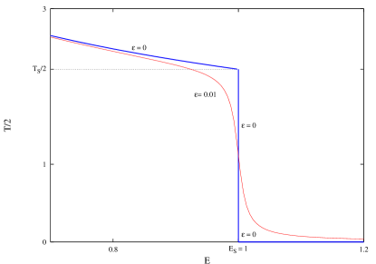
Figure 6: $T$ as function of $E$ for zero and nonzero $\epsilon$, thick and thin lines, respectively.

At ${E<1}$, the limit $\epsilon\to 0$ is straightforward. For ${E>1}$ a somewhat more careful analysis of the limit ${\epsilon\to 0}$ is needed. From Eq. (25) one observes that the limit ${\epsilon\to 0}$ with constant finite $T<\pi\sqrt{2}$ leads to solutions with $E=1$. Classical over-barrier solutions of the original problem with $E>E_{S}\equiv 1$ are obtained in the limit $\epsilon\to 0$ provided that $T$ also tends to zero while $\tau=T/\epsilon$ is kept finite. Different energies correspond to different values of $\tau$. And that is what one expects—classical over–barrier transitions are described by the solutions on the contour with $T\equiv 0$.

Let us now discuss the behavior of the branch points $t_{*}^{\pm}$ in complex time plane at small but finite $\epsilon$ and varying energy. A particularly interesting question is whether or not the singularities cross our time contour ABCD. The positions of the singularities in the regularized problem are (we set $\mathop{\mathrm{Re}}t_{0}=0$ here, see discussion after Eq. (18))

$$t_{*}^{\pm}=\frac{1}{\sqrt{2E}}\Bigg{\{}in\pi+i\frac{\pi}{2}+i\arg\left(\mathrm{e}^{-i\epsilon/2}\pm\sqrt{E}\right)\\ \pm\ln\left|\frac{\sqrt{E}+\mathrm{e}^{-i\epsilon/2}}{\sqrt{\mathrm{e}^{-i\epsilon}-E}}\right|\Bigg{\}}\;.$$

The behavior of the real parts of the “right” ($t_{*}^{+}$) and “left” ($t_{*}^{-}$) singularities is simple—as the energy approaches the barrier height, the singularities move towards large times, reaching a maximum distance from the origin equal to $\ln(2/\epsilon)/(2\sqrt{2})$ at $E=1$, and then move back. This again shows that our regularization makes the solutions continuous in energy. The behavior of the imaginary parts of the positions of the “right” singularities, $\mathop{\mathrm{Im}}(t_{*}^{+})$, is also simple: they scale with energy like $\pi/2\sqrt{2E}$ and stay essentially constant as energy crosses the value $E=1$. The imaginary parts of the positions of the “left” singularities, on the other hand, rapidly move down near $E=1$, together with the contour height $T/2$ (Fig. 5). So, the singularities do not cross the contour.

Thus, by introducing small parameter $\epsilon$, Eq. (23), we were able to regularize the system in such a way that the transition from classically forbidden region to the allowed one is rapid but smooth, and in the limit $\epsilon\to 0$ only the physically relevant branches of solutions are selected.

Although we have already studied all physically interesting solutions in non-regularized problem, let us analyze what happens in the limit $\epsilon\to 0$ to the regularized solutions with $0<T<\pi\sqrt{2}$ and $E=1$. At this point it is convenient to make the choice (19). Then in the limit $\epsilon\to 0$ one obtains a family of solutions with intermediate $T$,

$$\sinh X=-\mathrm{e}^{-\sqrt{2}\left(t-i\frac{T}{2}+c\right)}\;.$$ (26)

These solutions are no longer real at any finite time, but they are still real asymptotically, as $t\to+\infty$, where they approach the sphaleron, $X=0$. For all these solutions the suppression exponent (10) is zero.

Thus there are three different branches of solutions merging at each of the bifurcation points $E=1$, $T/2=0$ and $E=1$, $T/2=\pi/\sqrt{2}$. This is shown in Fig. 7.

Figure 7: The dependence of the period $T$ on energy $E$. Five branches of solutions are shown. A: represents tunneling solutions, Eq. (20), in the forbidden region ($E<V_{0}\equiv 1$); B: classically allowed transitions, $T=0$; (C and D): unphysical solutions undergoing reflection, in allowed and forbidden regions respectively; E new solutions (26).

We will see that a somewhat similar situation occurs in the case of multiple degrees of freedom, but there the branch analogous to the branch (26) is not degenerate in energy and is precisely the branch of relevant solutions in a certain region of parameters. The generalization of our regularization technique will enable us to select the physically relevant branches of solutions.

III Quantum mechanics of two degrees of freedom

The situation we discuss in this and the following section is a transition through a potential barrier of an oscillator whose spacing between the levels is much smaller than the barrier height. This model was already described in the Introduction, see (1) for the Hamiltonian.

As in the one dimensional case, we choose units with $\hbar=1,$ $m=1$. The oscillator frequency $\omega$ is of order $1$. The system is semiclassical, i.e.  conditions (2) are satisfied, if one chooses $\sigma=1/\sqrt{2\lambda}$, $V_{0}=1/\lambda$, where $\lambda$ is a small parameter. Note that $\lambda$ plays a role similar to $\hbar$, determining the magnitude of quantum fluctuations. At the classical level, this parameter is irrelevant: after rescaling the variables $x_{1}\to x_{1}/\sqrt{\lambda},\;\;x_{2}\to x_{2}/\sqrt{\lambda},$ the small parameter enters only through the overall multiplicative factor $1/\lambda$ in the Hamiltonian. Therefore, the semiclassical technique can be developed as an asymptotic expansion in $\lambda$.

The properties of the system described by the above Hamiltonian are made clearer by replacing the variables $x_{1},\;x_{2}$ with the center-of-mass coordinate $X\equiv(x_{1}+x_{2})/\sqrt{2}$ and the relative oscillator coordinate $y\equiv(x_{1}-x_{2})/\sqrt{2}$. In terms of the latter variables, the Hamiltonian takes the form

$$H=\frac{p_{X}^{2}}{2}+\frac{p_{y}^{2}}{2}+\frac{\omega^{2}}{2}y^{2}+\frac{1}{\lambda}\mathrm{e}^{-\lambda(X+y)^{2}/2}.$$ (27)

The interaction potential

$$V_{\mathrm{int}}\equiv\frac{1}{\lambda}\mathrm{e}^{-\lambda(X+y)^{2}/2}$$

vanishes in the asymptotic regions $X\to\pm\infty$ and describes a potential barrier between these regions. At $X\to\pm\infty$ the Hamiltonian (27) corresponds to an oscillator of frequency $\omega$ moving along the center-of-mass coordinate $X$. The oscillator asymptotic state may be characterized by its excitation number $N$ and total energy $E=\frac{p_{X}^{2}}{2}+\omega(N+1/2)$. We are interested in the transmissions through the potential barrier of the oscillator with given initial values of $E$ and $N$.

III.1 $T/\theta$ boundary value problem

The probability of tunneling from a state with fixed initial energy $E$ and oscillator excitation number $N$ from the asymptotic region $X\to-\infty$ to any state in the other asymptotic region $X\to+\infty$ takes the following form:

$$\mathcal{T}(E,N)=\lim_{t_{f}-t_{i}\to\infty}\sum_{f}\left|\langle f|\mathrm{e}^{-i\hat{H}(t_{f}-t_{i})}|E,N\rangle\right|^{2}\;,$$ (28)

where it is implicit that the initial and final states have support only well outside the range of the potential, with $X<0$ and $X>0$, respectively. Semiclassical methods are applicable when the initial energy and excitation number are parametrically large,

$$E=\tilde{E}/\lambda\;,\quad N=\tilde{N}/\lambda\;,$$

where $\tilde{E}$ and $\tilde{N}$ are held constant as $\lambda\to 0$. The transition probability has the exponential form

$${\cal T}=D\mathrm{e}^{-\frac{1}{\lambda}F(\tilde{E},\;\tilde{N})}\;,$$

where $D$ is a pre-exponential factor, which we do not consider in this paper. Our purpose is to calculate the leading semiclassical exponent $F(\tilde{E},\;\tilde{N})$. The exponent for tunneling from the oscillator ground state Rubakov:1992fb ; Rubakov:1992ec ; Bonini:1999fc may be obtained by taking $F(\tilde{E},\tilde{N})$ in the limit ${\tilde{N}\to 0}$.

The exponent $F(\tilde{E},\tilde{N})$ is again related to solutions of the complexified classical boundary value problem. The derivation is similar to that given in Sec. II.1; we present the details in App. A. The outcome is as follows. In addition to the Lagrange multiplier $T$ one now has another Lagrange multiplier $\theta$ which is related to the new parameter $N$ characterizing the incoming state. We again rescale the variables, $X\to X/\sqrt{\lambda}$, $y\to y/\sqrt{\lambda}$, and omit tilde over the rescaled quantities $\tilde{E},\;\tilde{N}$. As above, the boundary value problem is conveniently formulated on the contour ABCD in the complex time plane (see Fig. 3), with the imaginary part of the initial time equal to $T/2$. The coordinates $X(t),\;y(t)$ must satisfy the complexified equations of motion on the internal points of the contour, and be real in the asymptotic future (region D):

$$\frac{\delta S}{\delta X(t)}=\frac{\delta S}{\delta y(t)}=0\;,$$ (29a)

$$\begin{array}[]{l}\displaystyle\mathop{\mathrm{Im}}y(t)\to 0,\\[4.30554pt] \displaystyle\mathop{\mathrm{Im}}X(t)\to 0,\end{array}\qquad\text{as }t\to+\infty\;.$$ (29d)

In the asymptotic past (region A of the contour, where $$t=t^{\prime}+iT/2 t^{\prime} U_{\mathrm{int}}$$, is real negative) one can neglect the interaction potential , and the oscillator decouples:

$$y=\frac{1}{\sqrt{2\omega}}(u\mathrm{e}^{-i\omega t^{\prime}}+v\mathrm{e}^{i\omega t^{\prime}}).$$

The boundary conditions in the asymptotic past, $$t^{\prime}\to-\infty X$$, are that the center-of-mass coordinate must be real, while the complex amplitudes of the decoupled oscillator must be linearly related,

$$\begin{array}[]{l}\mathop{\mathrm{Im}}X\to 0,\\[4.30554pt] v\to\mathrm{e}^{\theta}u^{*},\end{array}\qquad\text{as }t^{\prime}\to-\infty\;.$$ (29e)

The boundary conditions (29d) and (29e) make, in fact, eight real conditions (since, e.g., $\mathop{\mathrm{Im}}X(t^{\prime})\to 0$ implies that both $\mathop{\mathrm{Im}}X$ and $\mathop{\mathrm{Im}}\dot{X}$ tend to zero), and completely determine a solution, up to time translation invariance (see discussion in App. A).

It is shown in App. A that a solution to this boundary value problem is, in fact, an extremum of the functional (cf. (10))

$$F[X,y;\;X^{*},y^{*};\;T,\theta]=-iS[X,y]+iS[X^{*},y^{*}]\\ -ET-N\theta+\text{Boundary terms}\;.$$ (30)

The value of this functional at the extremum gives the exponent for the transition probability

$$F(E,\;N)=2\mathop{\mathrm{Im}}S_{0}(T,\;\theta)-ET-N\theta\;,$$ (31)

where $S_{0}$ is the action of the solution (integrated by parts, see App. A),

$$S_{0}=\int\!dt\left(\!-\frac{1}{2}X\frac{d^{2}X}{dt^{2}}-\frac{1}{2}y\frac{d^{2}y}{dt^{2}}-\frac{1}{2}\omega^{2}y^{2}-U_{\mathrm{int}}(X,y)\right).$$

The values of the Lagrange multipliers $T$ and $\theta$ are related to energy and excitation number as follows,

$$E(T,\theta) = \frac{\partial}{\partial T}2\mathop{\mathrm{Im}}S_{0}(T,\theta)\;,$$ (32)

$$N(T,\theta) = \frac{\partial}{\partial\theta}2\mathop{\mathrm{Im}}S_{0}(T,\theta)\;.$$ (33)

Making use of Eq. (31), it is straightforward to check also the inverse Legendre transformation formulas,

$$T(E,\;N) = -\frac{\partial}{\partial E}F(E,\;N)\;,$$ (34)

$$\theta(E,\;N) = -\frac{\partial}{\partial N}F(E,\;N)\;.$$ (35)

One can also check that the right hand side of Eq. (32) coincides with the energy of the classical solution, while the right hand side of Eq. (33) is equal to the classical counterpart of the occupation number,

$$E=\frac{\dot{X}^{2}}{2}+\omega N\;;\qquad N=uv\;.$$ (36)

So, one may either search for the values of $T$ and $\theta$ that correspond to some given $E$ and $N$, or, following a computationally simpler procedure, solve the boundary value problem (29) for given $T$ and $\theta$ and then find the corresponding values of $E$ and $N$ from Eq. (36).

Let us discuss some subtle points of the boundary value problem (29). First, one notices that the condition of asymptotic reality (29d) does not always coincide with the condition of reality at finite time. Of course, if the solution approaches the asymptotic region $X\to+\infty$ on the part CD of the contour, the asymptotic reality condition (29d) implies that the solution is real at any finite positive $t$. Indeed, the oscillator decouples as $X\to+\infty$, so the condition (29d) means that its phase and amplitude, as well as $X(t)$, are real as $t\to+\infty$. Due to equations of motion, $X(t)$ and $y(t)$ are real on the entire CD–part of the contour. This situation corresponds to the transition directly to the asymptotic region $X\to+\infty$. However, the situation can be drastically different if the solution on the final part of the time contour remains in the interaction region. For example, let us imagine that the solution approaches the saddle point of the potential $X=0$, $y=0$ as $t\to+\infty$. Since one of the excitations about this point is unstable, there may exist solutions which approach this point exponentially along the unstable direction, i.e. $X(t),\;y(t)\propto\mathrm{e}^{-\mathrm{const}\cdot t}$ with possibly complex pre-factors. In this case the solution may be complex at any finite time, and become real only asymptotically, as $t\to+\infty$. Such solution corresponds to tunneling to the saddle point of the barrier, after which the system rolls down classically towards $X\to+\infty$ (with probability of order $1$, inessential for the tunneling exponent $F$). We will see in Sec. IV.1 that the situation of this sort indeed takes place for some values of energy and excitation number.

Second, since at large negative time (in the asymptotic region $X\to-\infty$) the interaction potential disappears, it is straightforward to continue the asymptotics of the solution to the real time axis. For solutions satisfying (29e) this gives at large negative time

$$y(t)=\frac{1}{\sqrt{2\omega}}\left(u\mathrm{e}^{-\frac{\omega T}{2}}\mathrm{e}^{-i\omega t}+u^{*}\mathrm{e}^{\theta+\frac{\omega T}{2}}\mathrm{e}^{i\omega t}\right)\;,$$

$$\mathop{\mathrm{Im}}X(t)=-i\frac{T}{2}p_{X}\;.$$

We see that the dynamical coordinates on the negative side of the real time axis are generally complex. For solutions approaching the asymptotic region $X\to+\infty$ as $t\to+\infty$ (so that $X$ and $y$ are exactly real at finite $t>0$), this means, in complete analogy to the one-dimensional case, that there should exist a branch point in the complex time plane: the contour in Fig. 3 winds around this point and cannot be deformed to the real time axis. This argument does not work for solutions ending in the interaction region as $t\to+\infty$, so branch points between the AB–part of the contour and the real time axis may be absent. We will see in Sec. IV.1 that this is indeed the case in our model for a certain range of $E$ and $N$.

III.2 Over-barrier transitions: boundary of the classically allowed region $E_{0}(N)$

Before studying the exponentially suppressed transitions, let us consider the classically allowed ones. To this end, let us study the classical evolution, in which the system is initially located at large negative $X$ and moves with positive center-of-mass velocity towards the asymptotic region $X\to+\infty$. The classical dynamics of the system is specified by four initial parameters. One of them (e.g., the initial center-of-mass coordinate) fixes the invariance under time translation, while the other three are the total energy $E$, the initial excitation number of the $y$–oscillator, defined in classical theory as $N\equiv E_{\mathrm{osc}}/\omega$, and the initial oscillator phase $\varphi_{i}$.

The classically allowed region is the region of the $E$–$N$ plane where over–barrier transitions are possible for some value(s) of the initial oscillator phase. For given $N$, at large enough $E$ the system can certainly evolve to the other side of the barrier. On the other hand, if $E$ is smaller than the barrier height, the system definitely undergoes reflection. Thus, there exists some boundary energy $E_{0}(N)$, such that classical transitions are possible for $E>E_{0}(N)$, while for $E<E_{0}(N)$ they do not occur for any initial phase $\varphi_{i}$. The line $E_{0}(N)$ represents the boundary of the classically allowed region. We have calculated $E_{0}(N)$ numerically for $\omega=0.5$: the result is shown in Fig. 2 and reproduced in Fig. 9

An important point of the boundary $E_{0}(N)$ corresponds to the static unstable classical solution $X(t)=y(t)=0$, the sphaleron (cf. Refs. Manton:1983nd ; Klinkhamer:1984di ). It is the saddle point of the potential $U(X,y)\equiv{\omega^{2}y^{2}}/{2}+U_{\mathrm{int}}(X,y)$ and has exactly one unstable direction, the negative mode (see Fig. 8). The sphaleron energy $E_{\mathrm{S}}=U(0,0)=1$ determines the minimum value of the function $E_{0}(N)$. Indeed, while classical over–barrier transitions with ${E<E_{\mathrm{S}}}$ are impossible, the over–barrier solution with slightly higher energy can be obtained as follows: at the point $X=y=0$, one adds momentum along the negative mode, thus “pushing” the system towards $X\to+\infty$. Continuing this solution backwards in time one finds that the system tends to $X\to-\infty$ for large negative time and has a certain oscillator excitation number. Solutions with energy closer to the sphaleron energy correspond to smaller “push” and thus spend longer time near the sphaleron. In the limiting case when the energy is equal to $E_{\mathrm{S}}$, the solution spends an infinite time in the vicinity of the sphaleron. This limiting case has a definite initial excitation number $N_{\mathrm{S}}$, so that $E_{0}(N_{\mathrm{S}})=E_{\mathrm{S}}$ (see Fig. 9). The value of $N_{\mathrm{S}}$ is unique because there is exactly one negative direction of the potential in the vicinity of the sphaleron.

In complete analogy to the features of the over–barrier classical solutions near the sphaleron point ($E_{\mathrm{S}}$, $N_{\mathrm{S}}$), one expects that as the values of $E,\;N$ approach any other boundary point $(E_{0}(N),\;N)$, the corresponding over–barrier solutions will spend more and more time in the interaction region, where $U_{\mathrm{int}}\neq 0$. This again follows from a continuity argument. Namely, let us first fix the initial and final times, $t_{i}$ and $t_{f}$. If in this time interval a solution with energy $E_{1}$ evolves to the other side of the barrier and a solution with energy $E_{2}$ and the same oscillator excitation number is reflected back, there exists an intermediate energy at which the solution ends up at $t=t_{f}$ in the interaction region. Taking the limit $t_{f}\to+\infty$ and $(E_{1}-E_{2})\to 0$, we obtain a point at the boundary of the classically allowed region and a solution tending asymptotically to some unstable time dependent solution that spends infinite time in the interaction region. We call the latter solution excited sphaleron; it describes some (in general nonlinear) oscillations above the sphaleron along the stable direction in coordinate space. Therefore, every point of the boundary ${(E_{0}(N),\;N)}$ corresponds to some excited sphaleron.

We display in Fig. 8 a solution, found numerically in our model, that tends to an excited sphaleron. We see that this trajectory is, roughly speaking, orthogonal to the unstable direction at the saddle point $({X=0,}\;{y=0})$.

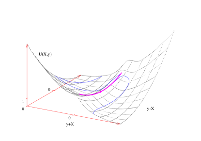
Figure 8: The potential (dotted lines) in the vicinity of the sphaleron ${(X=0,\;y=0)}$ (marked by the point), excited sphaleron (thick line) corresponding to the point $(E,N)=(1.985,3.72)$ at the boundary of the classically allowed region, and the trajectory of the solution which is close to this excited sphaleron (thin line). In this figure the asymptotic regions $X\to\pm\infty$ are along the diagonal.

III.3 Suppressed transitions: bifurcation line $E_{1}(N)$

Let us now turn to classically forbidden transitions, and consider the boundary value problem (29). It is relatively straightforward to obtain numerically solutions for $\theta=0$. The boundary conditions (29d), (29e) in this case take the form of reality conditions in the asymptotic future and past. It can be shown (see Ref. Khlebnikov:1991th ) that the physically relevant solutions with $\theta=0$ are real on the entire contour ABCD of Fig. 3 and describe nonlinear oscillations in the upside-down potential on the Euclidean part BC of the contour. The period of the oscillations is equal to $T$, so that the points B and C are two different turning points, where $\dot{X}=\dot{y}=0$. These real Euclidean solutions are called periodic instantons (see Ref. Khlebnikov:1991th ). A practical technique for obtaining these solutions numerically on the Euclidean part BC consists in minimizing the Euclidean action (for example with the method of conjugate gradients, see Ref. Bonini:1999cn for details). The solutions on the entire contour are then obtained by solving numerically the Cauchy problem, forward in time along the line CD and backward in time along the line BA. Having the solution in asymptotic past (region A), one then calculates its energy and excitation number (36). The solutions to this Cauchy problem are obviously real, so the boundary conditions (29d), (29e) are indeed satisfied with $\theta=0$. It is worth noting that solutions with $\theta=0$ are similar to the ones in quantum mechanics of one degree of freedom, see Fig. 4. The line of periodic instantons in $E$–$N$ plane in our model is shown in Fig. 9, again for $\omega=0.5$.

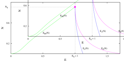
Figure 9: The boundary of the classically allowed region $E_{0}(N)$, the bifurcation line $E_{1}(N)$ and the line of the periodic instantons $E_{PI}(N)$.

Once the solutions with $\theta=0$ are found, it is natural to try to cover the entire classically forbidden region of the $E-N$ plane with a deformation procedure, by moving in small steps in $\theta$ (and $T$). The solution to the boundary value problem with $(T+\Delta T,\;\theta+\Delta\theta)$ may be obtained numerically, by applying an iteration technique, with the known solution at $(T,\;\theta)$ serving as the zeroth-order approximation. Provided the solutions have correct “topology” at each step, i.e. $X\to-\infty$ and $X\to+\infty$ on parts A and D of the contour, the solutions obtained by this “walking” procedure are physically relevant. However, the “walking” method fails to produce relevant solution if there are bifurcation points, where the physical branch of solutions merges to an unphysical branch. As there are unphysical solutions close to physical ones in the vicinity of a bifurcation point, one cannot “walk” near these points.

In our model, the walking method produces correct solutions to the $T/\theta$ boundary value problem in a large region of the $E-N$ plane, where $E<E_{1}(N)$. However, at sufficiently high energy $E>E_{1}(N)$, where $E_{1}(N)\gtrsim E_{\mathrm{S}}$, the deformation procedure generates solutions that bounce back from the barrier (see Fig. 10), i.e. have the wrong “topology”.

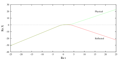
Figure 10: The dependence of the tunneling coordinate $X$ on time for two solutions with nearly the same energy and initial excitation number. The physical solution tunnels to the asymptotic region $X\to+\infty$, while the unphysical one gets reflected back to $X\to-\infty$. The physical solution has $E=1.028,\;N=0.44$, while the unphysical one has $E=1.034,\;N=0.44$. These two solutions are close to the point at the bifurcation line $E_{1}(N=0.44)=$ 1.031.

Clearly, the latter do not describe the tunneling transitions of interest. Therefore, if the semiclassical method is applicable at all in the region $E_{1}(N)<E<E_{0}(N)$, there exists another, physical branch of solutions. In that case the line $E_{1}(N)$ is the bifurcation line, where the physical solutions “meet” the ones with wrong “topology”. Walking in small steps in $\theta$ and $T$ is useless in the vicinity of this bifurcation line, and one needs to introduce some trick to find the relevant solutions beyond that line. The bifurcation line $E_{1}(N)$ for our quantum mechanical problem of two degrees of freedom with $\omega=0.5$ is shown in Fig. 9.

The loss of topology beyond a certain bifurcation line in $E-N$ plane is by no means a property of our model only. This phenomenon has been observed in field theory models, in the context of both induced false vacuum decay Kuznetsov:1997az and baryon-number violating transitions in gauge theory Bezrukov:2001dg (in field-theoretic models, the parameter $N$ is the number of incoming particles). In all cases, the loss of topology prevented one to compute the semiclassical exponent for the transition probability in an interesting region of relatively high energies, where the suppression of tunneling may be fairly weak.

Coming back to the quantum mechanics of two degrees of freedom, we point out that the properties of tunneling solutions approaching the bifurcation line $E_{1}(N)$ from the left, are in some sense similar to the properties of tunneling solutions in one-dimensional quantum mechanics near the boundary of the classically allowed region. Again by continuity, these solutions of our two-dimensional model spend a long time in the interaction region; this time tends to infinity on the line $E_{1}(N)$. Hence, on any point of this line, there is a solution that starts in the asymptotic region left of the barrier, and ends up on an excited sphaleron. We already mentioned in Sec. III.1 that such a behavior is indeed possible because of the existence of an unstable direction near the (excited) sphaleron, even for complex initial data. We have suggested in Sec. II.2 a trick to deal with this situation—this is our regularization technique.

IV Regularization technique

In this Section we further develop our regularization technique, and find the physically relevant solutions between the lines $E_{1}(N)$ and $E_{0}(N)$. We will see that all solutions from the new branch (and not only on the lines $E_{0}(N)$ and $E_{1}(N)$) correspond to tunneling onto the excited sphaleron. These solutions would be very difficult, if at all possible, to obtain directly, by solving numerically the non-regularized classical boundary value problem (29): they are complex at finite times, and become real only asymptotically as $t\to+\infty$, whereas numerical methods require working with finite time intervals.

As an additional advantage, our regularization technique enables one to obtain a family of the over–barrier solutions, that covers all the classically allowed region, including its boundary. This may be of interest in models with large number of degrees of freedom and in field theory, where finding the boundary of the classically allowed region by direct methods is difficult (see e.g., Ref. Rebbi:1995zw for discussion of this point).

IV.1 Regularized problem in the classically forbidden region

The main idea of our method is to “regularize” the equations of motion by adding a term proportional to a small parameter $\epsilon$ so that configurations staying for an infinite time near the sphaleron no longer exist among the solutions of the $T/\theta$ boundary value problem. After performing the regularization we explore all the classically forbidden region without crossing the bifurcation line. Taking then the limit ${\epsilon\to 0}$ we reconstruct the correct values of $F$, $E$ and $N$.

When formulating the regularization technique it is more convenient to work with the functional $F[X,y;X^{*},y^{*};T,\theta]$ itself rather than with the equations of motion. We slightly modify the form of $F$, Eq. (30), so that $F$ is no longer extremized by configurations approaching the excited sphalerons asymptotically. To achieve this, we add to the original functional (30) a new term of the form $2\epsilon T_{\mathrm{int}}$, where $T_{\mathrm{int}}$ estimates the time the solution “spends” in the interaction region. The parameter of regularization $\epsilon$ is the smallest one in the problem, so any regular extremum of the functional $F$ (the solution that spends finite time in the region $U_{\mathrm{int}}\neq 0$) changes only slightly after the regularization. At the same time, the excited sphaleron configuration has $T_{\mathrm{int}}=\infty$ which leads infinite value of the regularized functional $F_{\epsilon}\equiv F+2\epsilon T_{\mathrm{int}}$. Hence, the excited sphalerons are not stationary points of the regularized functional.

For the problem at hand, $U_{\mathrm{int}}\sim 1$ in the interaction region, and $T_{\mathrm{int}}$ can be defined as follows,

$$T_{\mathrm{int}}=\frac{1}{2}\left[\int dt\;U_{\mathrm{int}}(X,y)+\int dt\;U_{\mathrm{int}}(X^{*},y^{*})\right]\;.$$ (37)

We notice that $T_{\mathrm{int}}$ is real, and that the regularization is equivalent to the multiplication of the interaction potential by a complex factor

$$U_{\mathrm{int}}\to(1-i\epsilon)U_{\mathrm{int}}=\mathrm{e}^{-i\epsilon}U_{\mathrm{int}}+O(\epsilon^{2})\;.$$ (38)

This results in the corresponding change of the classical equations of motion, while the boundary conditions (29d), (29e) remain unaltered.

We still have to understand whether solutions with $\epsilon\neq 0$ exist at all. The reason for the existence of such solutions is as follows. Let us consider a well-defined (for $\epsilon>0$) matrix element

$$\mathcal{T}_{\epsilon}=\lim\limits_{t_{f}-t_{i}\to\infty}\sum\limits_{f}\left|\langle f|\mathrm{e}^{(-i\hat{H}-\epsilon U_{\mathrm{int}})(t_{f}-t_{i})}|E,N\rangle\right|^{2}\;,$$

where $|E,\;N\rangle$ denotes, as before, the incoming state with given energy and number of particles. The quantity ${\cal T}_{\epsilon}$ has a well defined limit as $\epsilon\to 0$, equal to the tunneling probability (28). As the saddle point of the regularized functional $F_{\epsilon}\equiv F+2\epsilon T_{\mathrm{int}}$ gives the semiclassical exponent for the quantity ${\cal T}_{\epsilon}$, one expects that such saddle point indeed exists.

Therefore, the regularized $T/\theta$ boundary value problem is expected to have solutions necessarily spending finite time in the interaction region. By continuity, these solutions do not experience reflection from the barrier, if one makes use of the “walking” procedure starting from solutions with correct “topology”. The line $E_{1}(N)$ is no longer a bifurcation line of the regularized system, so the walking procedure enables one to cover the entire forbidden region. The semiclassical suppression factor of the original problem is recovered in the limit $\epsilon\to 0$.

It is worth noting that the interaction time is Legendre conjugate to $\epsilon$,

$$T_{\mathrm{int}}=\frac{1}{2}\frac{\partial}{\partial\epsilon}F_{\epsilon}(E,N,\epsilon)\;.$$ (39)

Useful equations can also be obtained from Eqs. (32) and (33):

$$E = E|_{\epsilon=0}+2\epsilon\frac{\partial T_{\mathrm{int}}}{\partial T}+O(\epsilon)\;,$$ (40)

$$N = N|_{\epsilon=0}+2\epsilon\frac{\partial T_{\mathrm{int}}}{\partial\theta}+O(\epsilon)\;.$$ (41)

These equations show how the values of $E$ and $N$ change with $\epsilon$—away from the would-be bifurcation line $E_{1}(N)$ the values of $E$ and $N$ depend slightly on $\epsilon$, while at $E\sim E_{1}(N)$ where $T_{\mathrm{int}}$ takes large values (for small $\epsilon$), the dependence is strong and results in a considerable shift of the point $(E,N)$. Eqs. (39), (40), (41) may be used as a check of numerical calculations.

We implemented the regularization procedure numerically. To solve the boundary value problem, we make use of the computational methods described in Ref. Bonini:1999fc . In our calculations we used $\omega=0.5$. To obtain the semiclassical tunneling exponent in the region between the bifurcation line $E_{1}(N)$ and boundary of the allowed region, $E_{0}(N)$, we began with a solution to the non-regularized problem deep in the forbidden region (i.e., at $E<E_{1}(N)$). For that value of $T$ and $\theta$ we increased the value of $\epsilon$ from zero to a certain small positive number. Then we changed $T$ and $\theta$ in small steps, keeping $\epsilon$ finite, and found solutions to the regularized problem in the region $E_{1}(N)<E<E_{0}(N)$. These solutions had correct “topology”, i.e. they indeed ended up in the asymptotic region $X\to+\infty$. Finally, we lowered $\epsilon$ and extrapolated $F$, $E$ and $N$ to the limit $\epsilon\to 0$.

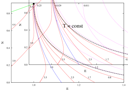
Figure 11: Lines $T=\mathrm{const}$ for $\epsilon=0.002$. Numbers near each line show the values of $T$. The boundary of the classically allowed region, the bifurcation line and the line of periodic instantons are shown by dashed lines.

The lines $T=\mathrm{const}$ for $\epsilon=0.002$ are shown in Fig. 11. We see that at $\epsilon\neq 0$ these lines are smooth and extend from $\theta=0$ (the line of periodic instantons) to $\theta=\infty$ (the line $N=0$). They indeed cover all the tunneling region without any irregularities at the bifurcation line $E_{1}(N)$.

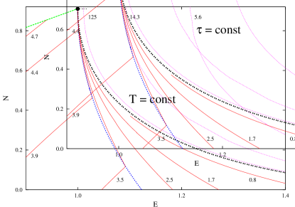
Figure 12: The lines $T=\mathrm{const}$ (in the forbidden region) and $\tau=\mathrm{const}$ (in the allowed region), see Sec. IV.3, in the limit $\epsilon\to 0$. Numbers near the lines are the values of $T$ and $\tau$.

The same lines $T=\mathrm{const}$, but now in the limit $\epsilon\to 0$ are shown in Fig. 12; the lines ${\theta=\mathrm{const}}$, again in the limit $\epsilon\to 0$, are presented in Fig. 13. It is seen that the functions $T(E,N)$ and $\theta(E,N)$ are continuous, while their first derivatives have discontinuities at the bifurcation line $E_{1}(N)$. As $T$ and $\theta$ are the derivatives of the tunneling exponent $F(E,N)$, see Eqs. (34), (35), the suppression exponent $F$ itself has discontinuities of the second derivatives only. The lines $F=\mathrm{const}$ are shown in Fig. 14. We see that the function $F$ and its first derivatives are indeed continuous.

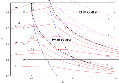
Figure 13: The lines $\theta=\mathrm{const}$ and $\vartheta=\mathrm{const}$ in the limit $\epsilon\to 0$. Numbers near the lines are the values of $\theta$ and $\vartheta$.

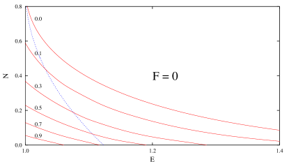
Figure 14: The lines $F=\mathrm{const}$ at energies above $E_{S}=1$. Dashed line shows $E_{1}(N)$.

Let us consider more carefully the solutions in the region $E_{1}(N)<E<E_{0}(N)$ which we obtain in the limit $\epsilon\to 0$. They belong to a new branch, and thus may exhibit new physical properties. Indeed, we found that, as the value of $\epsilon$ decreases to zero, the solution at any point $(E,N)$ with $E_{1}(N)<E<E_{0}(N)$ spends more and more time in the interaction region. The limiting solution corresponding to $\epsilon=0$ has infinite interaction time: in other words, it tends, as $t\to+\infty$, to one of the excited sphalerons. The resulting physical picture is that at large enough energy (i.e., at $E>E_{1}(N)$), the system prefers to tunnel exactly onto an unstable classical solution, excited sphaleron, that oscillates about the top of the potential barrier! To demonstrate this, we have plotted in Fig. 15 the solution $\vec{x}(t)\equiv(X(t),y(t))$ at large times, after taking numerically the limit $\epsilon\to 0$. To understand this figure, one recalls that the potential near the sphaleron point $X=y=0$ has one positive mode and one negative mode. Namely, by introducing new coordinates $c_{+}$, $c_{-}$,

$$X=\cos\alpha\;c_{+}+\sin\alpha\;c_{-}\;,$$

$$y=-\sin\alpha\;c_{+}+\cos\alpha\;c_{-}\;,$$

$$\mathrm{ctg}2\alpha=-\frac{\omega^{2}}{2}\;,$$

one writes, in the vicinity of the sphaleron,

$$H=1+\frac{p_{+}^{2}}{2}+\frac{p_{-}^{2}}{2}+\frac{\omega_{+}^{2}}{2}c_{+}^{2}-\frac{\omega_{-}^{2}}{2}c_{-}^{2}\;,$$

where

$$\omega_{\pm}=-1+\frac{\omega^{2}}{2}\pm\sqrt{1+\frac{\omega^{4}}{4}}\;.$$

Since the solutions to the $T/\theta$ boundary value problem are complex, the coordinates $c_{+}$ and $c_{-}$ are complex too. We show in Fig. 15 real and imaginary parts of $c_{+}$ and $c_{-}$ at large real time $t$ (part CD of the contour). We see that while $\mathop{\mathrm{Re}}c_{+}$ oscillates, the unstable coordinate $c^{-}$ approaches asymptotically the sphaleron value: $c_{-}\to 0$ as $t\to+\infty$. The imaginary part of $c_{-}$ is non-zero at any finite time. This is the reason for the failure of straightforward numerical methods in the region $E>E_{1}(N)$: the solutions from the physical branch do not satisfy the conditions of reality at any large but finite final time. We have pointed out in Sec. III.1 that this can happen only if the solution ends up near the sphaleron, which has a negative mode.

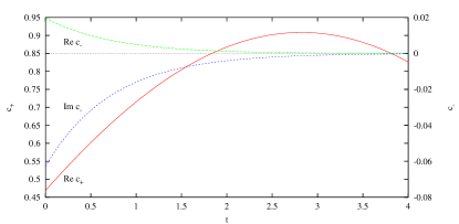
Figure 15: The large-time behavior of a solution with $\epsilon=0$ at $(E=1.05,\;N=0.43)$. The coordinates $X$ and $y$ are decomposed in a basis of the eigenmodes near the sphaleron. Note that $\mathop{\mathrm{Im}}c^{+}=0$.

It is interesting to compare the branches of solutions in the two– and one–dimensional models (the latter was discussed in Sec. II). The dependence $T(E)$ in these models is shown in Fig. 16 (for the two dimensional problem the graph corresponds to constant oscillator excitation number $N=0.1$). We see that the structure of the branches is similar, though in the one–dimensional case the solutions corresponding to “tunneling” onto the sphaleron are degenerate in energy and are not really useful for finding the transition exponent. In the two–dimensional model, on the other hand, the similar branch is the one relevant at $E_{1}(N)<E<E_{0}(N)$.

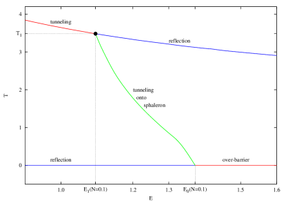
(a)

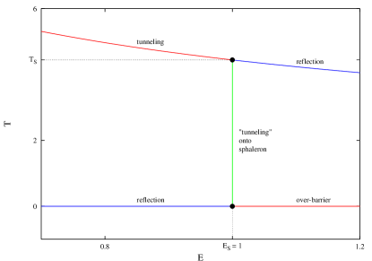
(b)

Figure 16: Dependence of the parameter $T=-\partial F/\partial E$ on energy for (a) the two dimensional model with fixed $N=0.1$ and (b)the one dimensional model. The lower picture is the same as Fig. 7. Different lines correspond to different branches of classical solutions to $T/\theta$ boundary value problem. The branches labelled “reflection” have wrong “topology”.

IV.2 Regularization technique versus exact quantum–mechanical solution

The quantum mechanics of two degrees of freedom is a convenient testing ground for checking the semiclassical methods Bonini:1999cn ; Bonini:1999kj and, in particular, our regularization technique. The solutions to the full stationary Schrödinger equation may be found numerically in this case at finite values of the semiclassical parameter $\lambda$, and the results may be extrapolated to $\lambda\to 0$. The suppression factor may be then compared to the semiclassical result. We performed this check in the region $E>E_{S}=1$, which is most interesting for our purposes. We applied the numerical techniques for solving the full stationary Schrödinger equation, which were developed in Ref. Bonini:1999kj ; our results agree with Ref. Bonini:1999kj where comparison is possible. The results of the full quantum mechanical calculation of the suppression exponent $F$ in the limit $\lambda\to 0$ are represented by points in Fig. 17. The lines in that figure represent the values, for constant $N$, of the semiclassical exponent $F(E,N)$, which we obtained by making use of the regularization procedure and extrapolation to $\epsilon\to 0$. We see that in the entire forbidden region (including the region $E>E_{1}(N)$) the semiclassical result for $F$ coincides with the exact one.

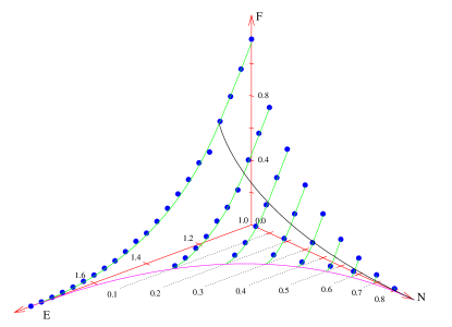
Figure 17: The tunneling exponent $F(E,N)$ in the region $E>E_{\mathrm{S}}=1$. The lines show the semiclassical results while points represent the exact ones, obtained by solving the Schrödinger equation. The lines across the plot are the boundary of the classically allowed region $E_{0}(N)$ and the bifurcation line $E_{1}(N)$.

IV.3 Classically allowed region

Finally, let us show that our regularization procedure enables one to obtain a subset of classical over–barrier solutions, that exist at high enough energies. This subset is interesting, as it extends all the way to the boundary of the classically allowed region, $E=E_{0}(N)$. In principle, finding this boundary is purely a problem of classical mechanics, and, indeed, in mechanics of two degrees of freedom one obtains this boundary numerically by solving numerically the Cauchy problem for given $E$ and $N$ and all possible oscillator phases, see Sec. III.2. However, if the number of degrees of freedom is much larger, this classical problem becomes quite complicated, as one has to span a high-dimensional space of Cauchy data. As an example, a stochastic Monte Carlo technique was developed in Ref. Rebbi:1995zw to deal with this problem in field theory context. The approach below may be viewed as an alternative to the Cauchy methods.

First, let us recall that all classical over–barrier solutions with given energy and excitation number satisfy the $T/\theta$ boundary value problem with $T=0$, $\theta=0$. We cannot reach the allowed region of $E-N$ plane without regularization, because we have to cross the line $E_{0}(N)$ corresponding to the excited sphaleron configurations in the final state. However, the excited sphalerons no longer exist among the solutions of the regularized boundary value problem at any finite value of $\epsilon$. This suggests that the regularization enables one to enter the classically allowed region and, after taking an appropriate limit, obtain classical solutions with finite values of $E$, $N$.

By definition, the classically allowed transitions have $F=0$. Thus, one expects that in the allowed region, the regularized problem has the property that $F_{\epsilon}(E,N)=\epsilon f(E,N)+O(\epsilon^{2})$. In view of the inverse Legendre formulas (34), (35) the values of $T$ and $\theta$ must be of order $\epsilon$: $T=\epsilon\tau(E,N)$, ${\theta=\epsilon\vartheta(E,N)}$, where the quantities $\tau$ and $\vartheta$ are related to the initial energy and excitation number (see Eq. (32), (33)) in the following way,

$$E = \lim\limits_{\epsilon\to 0}\frac{\partial}{\partial T}2\mathop{\mathrm{Im}}S_{\epsilon}=\frac{\partial}{\partial\tau}2T_{\mathrm{int}}(\tau,\vartheta)\;,$$ (42)

$$N = \lim\limits_{\epsilon\to 0}\frac{\partial}{\partial\theta}2\mathop{\mathrm{Im}}S_{\epsilon}=\frac{\partial}{\partial\vartheta}2T_{\mathrm{int}}(\tau,\vartheta),$$ (43)

and we have used the form (38) of the regularized potential. Therefore, one expects that one can invade the classically allowed region by taking a fairly sophisticated limit $\epsilon\to 0$ with $\tau\equiv T/\epsilon=\mathrm{const}$, $\vartheta\equiv\theta/\epsilon=\mathrm{const}$. In the allowed region the parameters $\tau$ and $\vartheta$ are analogous to $T$ and $\theta$.

By solving the regularized $T/\theta$ boundary value problem one constructs a single solution for given $E$ and $N$. On the other hand, for $\epsilon=0$ there are more classical over–barrier solutions: they form a continuous family labeled by the initial oscillator phase. Thus, after taking the limit $\epsilon\to 0$ one obtains a subset of over–barrier solutions, which should therefore obey some additional constraint. It is almost obvious, that this constraint is that the interaction time $T_{\mathrm{int}}$, Eq. (37), is minimal. This is shown in App. B.

The subset of classical over–barrier solutions obtained in the limit ${\epsilon\to 0}$ of the regularized $T/\theta$ procedure extends all the way to the boundary of the classically allowed region. Let us see what happens when one approaches this boundary from the classically allowed side. At the boundary $E_{0}(N)$, the unregularized solutions tend to excited sphalerons, so the interaction time $T_{\mathrm{int}}$ is infinite. This is consistent with (42), (43) only if $\tau$ and $\vartheta$ become infinite at the boundary. Thus, to obtain a point of the boundary one takes the further limit,

$$\big{(}E_{0}(N),\,N\big{)}=\lim_{\stackrel{{\scriptstyle\scriptstyle\tau/\vartheta=\mathrm{const}}}{{\scriptstyle\tau\to+\infty}}}\big{(}E(\tau,\vartheta),N(\tau,\vartheta)\big{)}\;.$$

Different values of $\tau/\vartheta$ correspond to different points of the line $E_{0}(N)$. In this way one finds the boundary of the classically allowed region without an initial-state simulation.

We have checked this procedure numerically. The line $\tau=\mathrm{const},\vartheta=\mathrm{const}$, with varying $\epsilon$, is shown in Fig. 18. The limit $\epsilon\to 0$ exists indeed—the values of $E$ and $N$ tend to the point (c) of the classically allowed region. The phase of the tunneling coordinate $X(t)$ in complex time plane is shown in Fig. 19 for the three points (a), (b) and (c) of the curve Fig. 18. The branch points of the solution, the cuts and the contour are clearly seen on these graphs.

It is worth noting that the left branch points $t_{-}^{*}$ move down as $T$ and $\theta$ approach zero. Solutions to the right of the point (b) (along the curve of Fig. 18) have left branch point in the lower complex half-plane, $\mathop{\mathrm{Im}}t^{*}_{-}<0$. Therefore, the corresponding contour may be continuously deformed to the real time axis. These solutions still satisfy the reality conditions asymptotically (see Fig. 15), but show nontrivial complex behavior at any finite time.

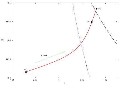
Figure 18: The line $\tau\equiv T/\epsilon=\mathrm{const}=380$, $\vartheta\equiv\theta/\epsilon=\mathrm{const}=130$ connecting the points (a): $T=3.8$, $\theta=1.3$, $\epsilon=0.01$ and (c): $T=0$, $\theta=0$, $\epsilon=0$. Point (b) in the middle has $T=1.82$, $\theta=0.62$, $\epsilon=0.0048$. As the values of $\tau$ and $\vartheta$ are quite large, the limiting point is close to the boundary of the classically allowed region. The reflection boundary and the boundary of the classically allowed region are shown by dashed lines.

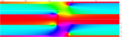
(a)

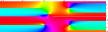
(b)

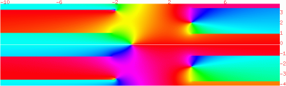
(c)

$\begin{array}[]{c}\pi\\ -\pi\end{array}\begin{array}[]{c}\includegraphics[width=28.45274pt]{fig18d}\end{array}0$

Figure 19: The phase of the tunneling coordinate in complex time plane at the three points of the curve $\tau=\mathrm{const}$, $\vartheta=\mathrm{const}$ (see Fig. 18). The asymptotics $X\to-\infty$ and $X\to+\infty$ correspond to $\mathrm{arg}(X)=\pi$ and $0$ correspondingly. The contour in the time plane is plotted with white line.

Making use of the regularized $T/\theta$ procedure, one is able to approach the boundary of the classically allowed region from both sides. The points at this boundary may be obtained by taking the limits $T\to 0,\;T/\theta=\mathrm{const}$ of the tunneling solutions and $\tau\to+\infty$, ${\tau/\vartheta=\mathrm{const}}$ of the classically allowed ones. As $\tau^{*}\equiv\tau/\vartheta=T/\theta$ by construction, the lines $\tau^{*}=\mathrm{const}$ are continuous at the boundary $E_{0}(N)$, though may have discontinuity of the derivatives. These lines are shown in Fig. 20. We see that the variable $\tau^{*}$ can be used to parametrize the curve $E_{0}(N)$.

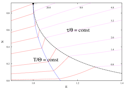
Figure 20: Lines $T/\theta=\mathrm{const}$ are continuously connected with the lines ${\tau/\vartheta=\mathrm{const}}$. The numbers near the lines give the values of $T/\theta=\tau/\vartheta$.

For completeness, the lines $\tau=\mathrm{const}$ and $\vartheta=\mathrm{const}$ in the classically allowed region are presented in Figs. 13, 14.

V Conclusions and Discussion

Though the semiclassical processes studied in this paper were dubbed “tunneling”, our results suggest somewhat different interpretation at energies exceeding the minimum height of the barrier, $E_{S}$. At these energies, it is energetically allowed that the system jumps above the barrier, and restarts its classical evolution from the region near its saddle point. This is precisely what we have observed. From the physical viewpoint, this is not quite what is normally meant by “tunneling through a barrier”. Yet the transitions remain exponentially suppressed (until the energy reaches the boundary of the allowed region), but, intuitively, the reason is different: to jump above the barrier, the system has to undergo considerable rearrangement, unless the incoming state is chosen properly (i.e. unless the oscillator excitation number in our model is large enough). This rearrangement costs exponentially small probability factor. We note that similar exponential factor was argued to appear in various field theory processes with multi-particle final states Banks:1990zb ; Zakharov:1991rp ; Veneziano:1992rp ; Rubakov:1995hq .

The $T/\theta$ boundary value problem, equipped with our regularization technique, enables one to deal with this situation, which, in the language of complex classical solutions, corresponds to a new physically relevant branch. The regularization procedure chooses automatically the correct branch, and thus provides an efficient way to cross the bifurcation lines where different branches merge. The phenomenon discussed in this paper appears to be quite general, as it exists in diverse quantum systems, from two-dimensional quantum mechanics to quantum field theory. The appropriate generalization of our regularized $T/\theta$ procedure is straightforward; we are going to report on this application to baryon–number violating processes in gauge theory in future publication BLRRT:prepare .

Appendix A $T/\theta$ boundary value problem

The semiclassical method for calculating the probability of tunneling from a state with a few parameters fixed was developed in Rubakov:1992ec ; Rubakov:1992fb ; Kuznetsov:1997az ; Bezrukov:2001dg in context of field theoretical models and in Bonini:1999kj ; Bonini:1999cn in quantum mechanics. Here we outline the method, adapted to our model of two degrees of freedom.

A.1 Path integral representation of the transition probability

We begin with the path integral representation for the probability of tunneling from the asymptotic region $X\to-\infty$ through a potential barrier. Let the incoming state $|E,\;N\rangle_{\delta}$ have fixed energy and oscillator excitation number, and has support only for $X\ll 0$, well outside the range of the potential barrier. The inclusive tunneling probability for states of this type is given by

$$\mathcal{T}(E,N)=\lim\limits_{t_{f}-t_{i}\to\infty}\Bigg{\{}\int\limits_{0}^{+\infty}dX_{f}\int\limits_{-\infty}^{+\infty}dy_{f}\\ \left|\langle X_{f},y_{f}|\mathrm{e}^{-i\hat{H}(t_{f}-t_{i})}|E,N\rangle\right|^{2}\Bigg{\}}\;.$$ (44)

This probability can be reexpressed in terms of the transition amplitudes

$${\cal A}_{fi}=\langle X_{f},\;y_{f}|\mathrm{e}^{-iH(t_{f}-t_{i})}|X_{i},\;y_{i}\rangle$$ (45)

and initial-state matrix elements

$${\cal B}_{ii^{\prime}}=\langle X_{i},\;y_{i}|E,\;N\rangle\langle E,\;N|X_{i}^{\prime},\;y_{i}^{\prime}\rangle$$ (46)

in the following way,

$${\cal T}(E,\;N)=\lim\limits_{t_{f}-t_{i}\to\infty}\Bigg{\{}\int\limits_{0}^{+\infty}dX_{f}\int\limits_{-\infty}^{0}d{X}_{i}\,d{X}_{i}^{\prime}\\ \int\limits_{-\infty}^{+\infty}dy_{i}\,dy_{i}^{\prime}\,dy_{f}\;{\cal A}_{fi}{\cal A}_{i^{\prime}f}^{*}{\cal B}_{ii^{\prime}}\Bigg{\}}\;.$$ (47)

The transition amplitude and its complex conjugate have the familiar path integral representation:

$$\mathcal{A}_{fi} = \int[d\vec{x}]\Bigg{|}_{\stackrel{{\scriptstyle\scriptscriptstyle\vec{x}(t_{i})=\vec{x}_{i}}}{{\scriptscriptstyle\vec{x}(t_{f})=\vec{x}_{f}}}}\mathrm{e}^{iS[\vec{x}]}\;,$$ (48)

$$\mathcal{A}_{i^{\prime}f}^{*} = \int[d\vec{x^{\prime}}]\Bigg{|}_{\stackrel{{\scriptstyle\scriptscriptstyle\vec{x}^{\prime}(t_{i})=\vec{x}^{\prime}_{i}}}{{\scriptscriptstyle\vec{x}^{\prime}(t_{f})=\vec{x}_{f}}}}\mathrm{e}^{-iS[\vec{x^{\prime}}]}\;,$$

where $\vec{x}=(X,y)$, and $S$ is the action of the model. To obtain a similar representation for the initial-state matrix elements let us rewrite ${\cal B}_{ii^{\prime}}$ as follows,

$${\cal B}_{ii^{\prime}}=\langle X_{i},\;y_{i}|\hat{P}_{E}\hat{P}_{N}|X_{i}^{\prime},\;y_{i}^{\prime}\rangle\;,$$ (49)

where $\hat{P}_{N}$ and $\hat{P}_{E}$ denote the projectors onto states with oscillator excitation number $N$ and total energy $E$ respectively. It is convenient to use the coherent state formalism for the $y$-oscillator and choose the momentum basis for the $X$-coordinate. In this representation, the kernel of the projector operator $\hat{P}_{E}\hat{P}_{N}$ takes the form

$$\langle q,\;b|\hat{P}_{E}\hat{P}_{N}|p,\;a\rangle=\frac{1}{(2\pi)^{2}}\int d\xi\,d\eta\\ \mathrm{exp}\left(-iE\xi-iN\eta+\frac{i}{2}p^{2}\xi+\mathrm{e}^{i\omega\xi+i\eta}\bar{b}a\right)\delta(q-p)\;,$$

where $|p,\;a\rangle$ is the eigenstate of the center-of-mass momentum $\hat{p}_{X}$ and $y$-oscillator annihilation operator $\hat{a}$ with eigenvalues $p$ and $a$ respectively. It is straightforward to express this matrix element in the coordinate representation using the formulas

$$\langle y|a\rangle = \sqrt[4]{\frac{\omega}{\pi}}\mathrm{e}^{-\frac{1}{2}a^{2}+\sqrt{2\omega}ay-\frac{1}{2}\omega y^{2}}\;,$$

$$\langle X|p\rangle = \frac{1}{\sqrt{2\pi}}\mathrm{e}^{ipX}\;.$$

Evaluating the Gaussian integrals over $a$, $b$, $p$, $q$, we obtain

$${\cal B}_{ii^{\prime}} = \int d\xi\;d\eta\;\mathrm{exp}\left(-iE\xi-iN\eta-\frac{i}{2}\frac{(X_{i}-X_{i}^{\prime})^{2}}{\xi}\right.$$ (50)

$$+\left.\frac{\omega}{1-\mathrm{e}^{-2i\omega\xi-2i\eta}}\left[\frac{y_{i}^{2}+y_{i}^{\prime 2}}{2}(1+\mathrm{e}^{-2i\omega\xi-2i\eta})\right.\right.$$

$$\quad\quad\quad\quad\quad\quad\quad\quad\quad-2y_{i}y_{i}^{\prime}\mathrm{e}^{-i\omega\xi-i\eta}\bigg{]}\bigg{)}$$

where we omit the pre-exponential factor depending on $\eta,\;\xi$. For the subsequent formulation of the boundary value problem it is convenient to introduce the notation

$$T=-i\xi\;,\qquad\theta=-i\eta\;.$$

Then, combining together the integral representations (50) and (48) and rescaling coordinates, energy and excitation number $\vec{x}\to\vec{x}/\sqrt{\lambda}$, $E\to E/\lambda$, $N\to N/\lambda$, we finally obtain

$${\cal T}(E,\;N)=\lim\limits_{t_{f}-t_{i}\to\infty}\Bigg{\{}\int\limits_{-i\infty}^{+i\infty}dT\;d\theta\int\;[d\vec{x}\;d\vec{x}^{\prime}]\\ \exp\left\{-\frac{1}{\lambda}F[\vec{x},\;\vec{x}^{\prime};\;T,\;\theta]\right\}\Bigg{\}}\;,$$ (51)

where

$$F[\vec{x},\;\vec{x}^{\prime};\;T,\;\theta]=-iS[X,y]+iS[X^{\prime},\;y^{\prime}]\\ -ET-N\theta+B_{i}(\vec{x}_{i},\vec{x^{\prime}}_{i};T,\theta).$$ (52)

Here the non-trivial initial term $B_{i}$ is

$$B_{i}=\ \frac{(X_{i}-X_{i}^{\prime})^{2}}{2T}$$

$$-\frac{\omega}{1-\mathrm{e}^{2\omega T+2\theta}}\bigg{[}\frac{1}{2}(y_{i}^{2}+{y_{i}^{\prime}}^{2})(1+\mathrm{e}^{2\omega T+2\theta})$$

$$\hphantom{-\frac{\omega}{1-\mathrm{e}^{2\omega T+2\theta}}\bigg{[}}-2y_{i}y_{i}^{\prime}\mathrm{e}^{\omega T+\theta}\bigg{]}\;.$$ (53)

In (51) $\vec{x}$ and $\vec{x^{\prime}}$ are independent integration variables, while $\vec{x}_{f}^{\prime}\equiv\vec{x}_{f}$, see Eqs. (47).

A.2 The boundary value problem

For small $\lambda$, the path integral (51) is dominated by a stationary point of the functional $F$. Thus, to calculate the tunneling exponent, we extremize this functional with respect to all variables of integration: $X(t)$, $y(t)$, $X^{\prime}(t)$, $y^{\prime}(t)$, $T$, $\theta$. Note that because of the limit $t_{f}-t_{i}\to+\infty$, the variation with respect to the initial and final values of coordinates leads to boundary conditions imposed at asymptotic $t\to\pm\infty$, rather than at finite times $t_{i},t_{f}$. Note also that the stationary points may be complex.

The variation of the functional (52) with respect to the coordinates at intermediate times gives second order equations of motion, in general complexified,

$$\frac{\delta S}{\delta X(t)}=\frac{\delta S}{\delta y(t)}=\frac{\delta S^{\prime}}{\delta X^{\prime}(t)}=\frac{\delta S^{\prime}}{\delta y^{\prime}(t)}=0\;.$$ (54a)

The boundary conditions at the final time $$t_{f}\to+\infty F X_{f}\equiv X_{f}^{\prime} y_{f}\equiv y_{f}^{\prime}$$ are obtained by extremization of with respect to , . These are

$$\dot{X_{f}}=\dot{X_{f}^{\prime}}\;,\qquad\dot{y_{f}}=\dot{y_{f}^{\prime}}\;.$$ (54b)

It is convenient to write the conditions at the initial time (obtained by varying $$X_{i} y_{i} X_{i}^{\prime} y_{i}^{\prime} t_{i}\to-\infty X\to-\infty$$, , , ) in terms of the asymptotic quantities. At the initial moment of time , the system moves in the region , well outside of the range of the potential barrier. Equations (54a) in this region describe free motion of decoupled oscillator, and the general solution takes the following form,

$$X(t)=X_{i}+p_{i}(t-t_{i}),$$

$$y(t)=\frac{1}{\sqrt{2\omega}}\left[a\mathrm{e}^{-i\omega(t-t_{i})}+\bar{a}\mathrm{e}^{i\omega(t-t_{i})}\right]\;,$$

while the solution for $$X^{\prime}(t) y^{\prime}(t) a \bar{a} X_{i} p_{i} a \bar{a}$$, has similar form. For the moment, and are independent variables. The initial boundary conditions in terms of the asymptotic variables , , , take the form:

$$p_{i}=p_{i}^{\prime}=-\frac{X_{i}-X_{i}^{\prime}}{iT},$$

$$a^{\prime}+\bar{a}^{\prime}=a\mathrm{e}^{\omega T+\theta}+\bar{a}\mathrm{e}^{-\omega T-\theta}\;,$$ (54c)

$$a+\bar{a}=a^{\prime}\mathrm{e}^{-\omega T-\theta}+\bar{a}^{\prime}\mathrm{e}^{\omega T+\theta}\;.$$

The variation with respect to the Lagrange multipliers $$T \theta E N$$ and gives the relation between the values of , and initial asymptotic variables (here we use the boundary conditions (54c)),

$$E = \frac{p_{i}^{2}}{2}+\omega N\;,$$ (54d)

$$N = a\bar{a}\;.$$

Equations (54a) – (54d) constitute the complete set of saddle-point equations for the functional $$F$$.

The variables $X^{\prime}$ and $y^{\prime}$ originate from the conjugate amplitude ${\cal A}_{i^{\prime}f}^{*}$ (see Eq. (48)), which suggests that they are the complex conjugate to $X$, $y$. Indeed, the Ansatz ${X^{\prime}(t)=X^{*}(t)}$, ${y^{\prime}(t)=y^{*}(t)}$ is compatible with the boundary value problem (54). Then the Lagrange multipliers $T$, $\theta$ are real, and the problem (54) may be conveniently formulated at the contour ABCD in the complex time plane (see Fig. 3).

Now we have only two independent complex variables $X(t)$ and $y(t)$, that have to satisfy the classical equations of motion in the interior of the contour,

$$\frac{\delta S}{\delta X(t)}=\frac{\delta S}{\delta y(t)}=0\;.$$ (55a)

The final boundary conditions (see Eq. (54b)) become the conditions of the reality of the variables $$X(t) y(t)$$ and at the asymptotic part D of the contour:

$$\begin{array}[]{l}\mathop{\mathrm{Im}}X_{f}=0,\;\;\mathop{\mathrm{Im}}y_{f}=0\;,\\[4.30554pt] \mathop{\mathrm{Im}}\dot{X}_{f}=0\;\;\mathop{\mathrm{Im}}\dot{y}_{f}=0\;,\end{array}\qquad t\to+\infty\;.$$ (55d)

The seemingly complicated initial conditions (54c) simplify when written in terms of the time coordinate $$t^{\prime}=t+iT/2$$ running along the part AB of the contour. Let us again write the asymptotics of a solution, but now along the initial part AB of the contour:

$$X=X_{0}+p_{0}(t^{\prime}-t_{i})\;,$$

$$y=\frac{1}{\sqrt{2\omega}}\left[u\mathrm{e}^{-i\omega(t^{\prime}-t_{i})}+v\mathrm{e}^{i\omega(t^{\prime}-t_{i})}\right]\;.$$

In terms of $$X_{0} y_{0} u v$$, , and , the boundary conditions (54c) are

$$\mathop{\mathrm{Im}}X_{0}=0,\;\;\mathop{\mathrm{Im}}p_{0}=0\;,$$ (55e)

$$v=u^{*}\mathrm{e}^{\theta}\;.$$

Finally, we write Eqs. (54d) in terms of the asymptotic variables along the initial part of the contour:

$$E=\frac{p_{0}^{2}}{2}+\omega N\;,$$ (56)

$$N=\omega uv\;.$$

These equations determine the Lagrange multipliers $T,\;\theta$ in terms of $E$, $N$. Alternatively, we can solve the problem (55) for given values of $T$, $\theta$ and find the values of $E$,$N$ from Eqs. (56), what is more convenient computationally.

Given a solution to the problem (55), the exponent $F$ is the value of the functional (52) at this saddle point. Explicitly

$$F=-ET-N\theta+2\mathop{\mathrm{Im}}S_{0}(T,\theta)\;,$$ (57)

where $S_{0}$ is the action of the system, integrated by parts

$$S_{0}=\int\!dt\left[-\frac{1}{2}X\frac{d^{2}}{dt^{2}}X-\frac{1}{2}y\frac{d^{2}}{dt^{2}}y-\frac{\omega^{2}}{2}y^{2}-U_{\mathrm{int}}(X,y)\right].$$

Note that we did not make use of the constraints (56) to obtain the formula (57), so we still can extremize (57) with respect to $T$ and $\theta$ (see discussion in Sec. III.1).

The classical problem (55) is conveniently dubbed $T/\theta$ boundary value problem. Eqs. (55d) and (55e) imply eight real boundary conditions for two complex second-order differential equations (55a). However, one of these real conditions is redundant: Eq. (55d) implies that the (conserved) energy is real, so the condition $\mathop{\mathrm{Im}}p_{0}\to 0$ is automatically satisfied (note that the oscillator energy $E_{\mathrm{osc}}=\omega uv=\omega\mathrm{e}^{\theta}uu^{*}$ is real). On the other hand, the system (55) is invariant under time translations along the real axis. This invariance may be fixed, e.g., by demanding that $\mathop{\mathrm{Re}}(X)$ takes a prescribed value at a prescribed large negative time $t^{\prime}_{0}$ (note that other ways may be used instead. In particular, for $E<E_{1}(N)$ it is convenient to impose the constraint $\mathop{\mathrm{Re}}\dot{X}({t=0})=0$). Together with the latter requirement, we have exactly eight real boundary conditions for the system of two complexified (i.e. four real) second-order equations.

Appendix B A property of solutions to $T/\theta$ problem in the allowed region

For given $E$, $N$ there is only one over–barrier classical solution which is obtained in the limit $\epsilon\to 0$ of the regularized $T/\theta$ procedure. To see what singles out this solution, let us analyze the regularized functional

$$F_{\epsilon}[q]=F[q]+2\epsilon T_{\mathrm{int}}[q],$$ (58)

where $q$ denotes the variables $\vec{x}(t),\;\vec{x}^{\prime}(t)$ and $T,\;\theta$ together. The unregularized functional $F$ has a valley of extrema $q^{e}(\varphi)$ corresponding to different values of the initial oscillator phase $\varphi$. Clearly, at small $\epsilon$ the extremum of $F_{\epsilon}$ is close to a point in this valley with the phase extremizing $T_{\mathrm{int}}[q^{e}(\varphi)]$.

$$\frac{d}{d\varphi}T_{\mathrm{int}}[q^{e}(\varphi)]=0\;.$$ (59)

Hence, the solution $q^{e}_{\epsilon}$ of the regularized $T/\theta$ boundary value problem tends to the over–barrier classical solution, with $T_{\mathrm{int}}$ extremized with respect to the initial oscillator phase.

Because $U_{\mathrm{int}}(\vec{x})>0$, $T_{\mathrm{int}}$ is a positive quantity with at least one minimum. In normal situation there is only one saddle point of $F_{\epsilon}$, so by solving the $T/\theta$ boundary value problem one obtains the classical solution with the time of interaction minimized.

The dependence of the interaction time on the initial oscillator phase for given values of energy and excitation number is shown in Fig. 21. We see that $T_{\mathrm{int}}$ indeed has one minimum, and the corresponding solution indeed coincides with the limit of the solution of the regularized $T/\theta$ boundary value problem (black point on the graph).

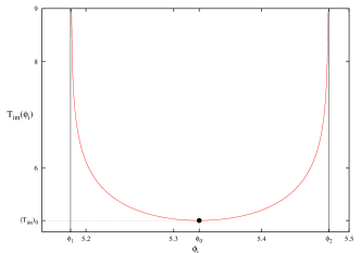
Figure 21: The dependence of the interaction time $T_{\mathrm{int}}$ on the initial oscillator phase at fixed values of $E$ and $N$, corresponding to the point (c) in Fig. 19. The black point marks the initial oscillator phase and interaction time calculated on the solution (c).

References

- (1) A. N. Kuznetsov and P. G. Tinyakov, Phys. Rev. D56, 1156 (1997), [hep-ph/9703256].
- (2) F. Bezrukov, C. Rebbi, V. Rubakov and P. Tinyakov, hep-ph/0110109.
- (3) W. H. Miller, Adv. Chem. Phys. 25, 69 (1974).
- (4) G. ’t Hooft, Phys. Rev. D14, 3432 (1976).
- (5) A. Ringwald, Nucl. Phys. B330, 1 (1990).
- (6) O. Espinosa, Nucl. Phys. B343, 310 (1990).
- (7) F. L. Bezrukov, D. Levkov, C. Rebbi, V. A. Rubakov and P. Tinyakov, In preparation (2003).
- (8) G. F. Bonini, A. G. Cohen, C. Rebbi and V. A. Rubakov, Phys. Rev. D60, 076004 (1999), [hep-ph/9901226].
- (9) G. F. Bonini, A. G. Cohen, C. Rebbi and V. A. Rubakov, quant-ph/9901062.
- (10) F. R. Klinkhamer and N. S. Manton, Phys. Rev. D30, 2212 (1984).
- (11) V. A. Rubakov, D. T. Son and P. G. Tinyakov, Phys. Lett. B287, 342 (1992).
- (12) V. A. Rubakov and P. G. Tinyakov, Phys. Lett. B279, 165 (1992).
- (13) G. F. Bonini et al., hep-ph/9905243.
- (14) N. S. Manton, Phys. Rev. D28, 2019 (1983).
- (15) S. Y. Khlebnikov, V. A. Rubakov and P. G. Tinyakov, Nucl. Phys. B367, 334 (1991).
- (16) C. Rebbi and J. Robert Singleton, hep-ph/9502370.
- (17) T. Banks, G. Farrar, M. Dine, D. Karabali and B. Sakita, Nucl. Phys. B347, 581 (1990).
- (18) V. I. Zakharov, Phys. Rev. Lett. 67, 3650 (1991).
- (19) G. Veneziano, Mod. Phys. Lett. A7, 1661 (1992).
- (20) V. A. Rubakov, hep-ph/9511236.