Additivity of Entanglement of Formation
of Two Three-level-antisymmetric States

Abstract

Quantum entanglement is the quantum information processing resource. Thus it is of importance to understand how much of entanglement particular quantum states have, and what kinds of laws entanglement and also transformation between entanglement states subject to. Therefore, it is essentialy important to use proper measures of entanglement which have nice properties. One of the major candidates of such measures is ”entanglement of formation”, and whether this measurement is additive or not is an important open problem. We aim at certain states so-called ”antisymmetric states” for which the additivity are not solved as far as we know, and show the additivity for two of them.

Keywords: quantum entanglement, entanglement of formation, additivity of entanglement measures, antisymmetric states.

1 Introduction

Concerning the additivity of entanglement of formation, only a few results have been known. Vidal et al. [1] showed that additivity holds for some mixture of Bell states and other examples by reducing the argument of additivity of the Holevo capacity of so-called ”entanglement breaking quantum channels” [2] and they are the non-trivial first examples. Matsumoto et al. [3] showed that additivity of entanglement of formation holds for a family of mixed states by utilizing the additivity of Holevo capacity for unital qubit channels [4] via Stinespring dilation [5].

In this extended abstract we prove that entanglement of formation is additive for tensor product of two three-dimensional bipartite antisymmetric states with a sketch of the proof. We proved by combination of elaborate calculations.

2 New additivity result

2.1 Antisymmetric states

Let us start with an introduction of our notations and concepts. $\mathcal{H}_{-}$ will stand for an antisymmetric Hilbert space, which is a subspace of a bipartite Hilbert space $\mathcal{H}_{AB}:=\mathcal{H}_{A}\otimes\mathcal{H}_{B}$, where both $\mathcal{H}_{A}$ and $\mathcal{H}_{B}$ are $3-$dimensional Hilbert spaces, spanned by basic vectors $\{{|{i}\rangle}\}_{i=1}^{3}$. $\mathcal{H}_{-}$ is three-dimensional Hilbert space, spanned by states $\{{|{i,j}\rangle}\}_{ij=23,31,12}$, where the state ${|{i,j}\rangle}$ is defined as $\frac{{|{i}\rangle}{|{j}\rangle}-{|{j}\rangle}{|{i}\rangle}}{\sqrt{2}}$. The space $\mathcal{H}_{-}$ is called antisymmetric because by swapping the position of two qubits in any of its states ${|{\psi}\rangle}$ we get the state $-{|{\psi}\rangle}$. Let $\mathcal{H}_{-}^{\otimes{n}}$ be the tensor product of $n$ copies of $\mathcal{H}_{-}$. These copies will be discriminated by the upper index as $\mathcal{H}_{-}^{(j)}$, for $j=1\ldots n$. $\mathcal{H}_{-}^{(j)}$ will then be an antisymmetric subspace of $\mathcal{H}_{A}^{(j)}\otimes\mathcal{H}_{B}^{(j)}$.

2.2 The result and proof sketch

It has been shown in [1] that $E_{f}(\rho)=1$ for any mixed state $\rho\in\mathcal{S}({\mathcal{H}_{-}})$. This result will play the key role in our proof. We prove now that :

Theorem .

$$E_{f}(\rho_{1}\otimes\rho_{2})=E_{f}(\rho_{1})+E_{f}(\rho_{2})\,\left(=2\right)$$ (1)

for any ${\rho_{1},\rho_{2}\in\mathcal{S}({\mathcal{H}_{-}})}$.

Proof.

To prove this theorem, it is sufficient to show that

$$E_{f}(\rho_{1}\otimes\rho_{2})\geq 2$$ (2)

since the subadditivity $E_{f}(\rho_{1}\otimes\rho_{2})\leq E_{f}(\rho_{1})+E_{f}(\rho_{2})=2$ is trivial. Indeed, it holds

$$E_{f} \!\!\!\!(\rho_{1}\otimes\rho_{2})=\inf\sum p_{i}E({|{\psi_{i}}\rangle}\!{\langle{\psi_{i}}|})$$ (3)

$$\leq \!\!\!\!\inf\sum p_{i}^{(1)}p_{i}^{(2)}E({|{\psi_{i}^{(1)}}\rangle}\!{\langle{\psi_{i}^{(1)}}|}\otimes{|{\psi_{i}^{(2)}}\rangle}\!{\langle{\psi_{i}^{(2)}}|})$$

$$= \!\!\!\!\inf\sum p_{i}^{(1)}E({|{\psi_{i}^{(1)}}\rangle}\!{\langle{\psi_{i}^{(1)}}|})$$

$$+\inf\sum p_{i}^{(2)}E({|{\psi_{i}^{(2)}}\rangle}\!{\langle{\psi_{i}^{(2)}}|})$$

$$= \!\!\!\!E_{f}(\rho_{1})+E_{f}(\rho_{2})$$

where $(p_{i}^{(j)},{|{\psi_{i}^{(j)}}\rangle})$ are subject to the condition of $\rho_{j}=\sum_{i}p_{i}^{(j)}{|{\psi_{i}^{(j)}}\rangle}\!{\langle{\psi_{i}^{(j)}}|}$. To prove (2), we first show that

$$E({|{\psi}\rangle}\!{\langle{\psi}|})\geq 2,\text{ for any pure state }{|{\psi}\rangle}\in{\mathcal{H}_{-}^{\otimes{2}}}.$$ (4)

Using the Schmidt decomposition, the state ${|{\psi}\rangle}$ can be decomposed as follows:

$${|{\psi}\rangle}=\sum\limits_{i=1}^{3}\sqrt{p_{i}}\>{|{\psi_{i}^{(1)}}\rangle}\otimes{|{\psi_{i}^{(2)}}\rangle},$$ (5)

where $p_{1},p_{2},p_{3}>0,p_{1}+p_{2}+p_{3}=1$, and $\{{|{\psi_{i}^{(j)}}\rangle}\}_{i=1}^{3}$ is an orthonormal basis of the Hilbert space $\mathcal{H}_{-}^{(j)}$, for $j=1,2$. Note that this Schmidt decomposition is with respect to $\mathcal{H}_{-}^{(1)}:\mathcal{H}_{-}^{(2)}$, or, it could be said that with respect to $\left(\mathcal{H}_{A}^{(1)}\otimes\mathcal{H}_{B}^{(1)}\right):\left(\mathcal{H}_{A}^{(2)}\otimes\mathcal{H}_{B}^{(2)}\right)$, not with respect to $\left(\mathcal{H}_{A}^{(1)}\otimes\mathcal{H}_{A}^{(2)}\right):\left(\mathcal{H}_{B}^{(1)}\otimes\mathcal{H}_{B}^{(2)}\right)$, where “:” indicates how to separate the system into two subsystems for the decomposition.

First, we will use the following fact.

Lemma .

If $\{{|{\psi_{i}}\rangle}\}_{i=1}^{3}$ is an orthonormal basis of $\mathcal{H}_{-}$, then there exists an unitary operator $U$, acting on both $\mathcal{H}_{A}$ and $\mathcal{H}_{B}$, such that $U\otimes U$ maps the states ${|{\psi_{1}}\rangle},{|{\psi_{2}}\rangle},{|{\psi_{3}}\rangle}$ into the states ${|{2,3}\rangle},{|{3,1}\rangle},{|{1,2}\rangle}$, respectively.

Therefore, by this Lemma Lemma, there exist unitary operators $U^{(1)},U^{(2)}$ such that

$$\begin{split}\big{(}U^{(1)}&\otimes U^{(1)}\otimes U^{(2)}\otimes U^{(2)}\big{)}{|{\psi}\rangle}\hfill\\ &=\sum\limits_{{i,j}\atop{ij=23,31,12}}\sqrt{p_{ij}}\>{|{i,j}\rangle}\otimes{|{i,j}\rangle}\;=:\;{|{\psi^{\prime}}\rangle},\end{split}$$ (6)

where $p_{23}:=p_{1},\;p_{31}:=p_{2},\;p_{12}:=p_{3}$.

As is written in the following, we use the following fact.

Lemma .

$$E({|{\psi^{\prime}}\rangle}\!{\langle{\psi^{\prime}}|})\geq 2,\quad\text{ if }\quad\begin{cases}\quad p_{23},p_{31},p_{12}\geq 0\\ \phantom{p_{1}}p_{23}+p_{31}+p_{12}=1\end{cases}.$$ (7)

(We proved this lemma by solving a cubic equation and bounding the Shannon entropy function with polynomial functions.) Local unitary operators do not change von Neumann reduced entropy, and therefore $E({|{\psi}\rangle}\!{\langle{\psi}|})=E({|{\psi^{\prime}}\rangle}\!{\langle{\psi^{\prime}}|})\geq 2$. That is, the claim (4) is proven.

We are now almost done. Indeed, the entanglement of formation is defined as

$$E_{f}(\rho)=\!\!\inf_{[(p_{i},\psi_{i})]_{i}\in{\Delta(\rho)}}\sum_{i}p_{i}E({|{\psi_{i}}\rangle}\!{\langle{\psi_{i}}|})$$ (8)

where

$$\Delta(\rho)=\left\{\left[(p_{i},\psi_{i})\right]_{i}\Bigm{|}\!\!\begin{array}[]{l}\sum_{i}p_{i}=1,p_{i}>0\forall i\\ \sum_{i}p_{i}{|{\psi_{i}}\rangle}\!{\langle{\psi_{i}}|}=\rho,\langle{\psi_{i}}|{\psi_{i}}\rangle=1\forall i\!\!\end{array}\right\}$$

and it is known that all ${|{\psi_{i}}\rangle}$ induced from $\Delta(\rho)$ satisfy ${|{\psi_{i}}\rangle}\in\mathop{\mathrm{Range}}\nolimits(\rho)$, where $\mathop{\mathrm{Range}}\nolimits(\rho)$ is sometimes called the image space of the matrix $\rho$, which is the set of $\rho{|{\psi}\rangle}$ with ${|{\psi}\rangle}$ running over the domain of $\rho$. Hence

$$E_{f}(\rho)\geq\inf\left\{E({|{\psi}\rangle}\!{\langle{\psi}|})\bigm{|}{|{\psi}\rangle}\in\mathop{\mathrm{Range}}\nolimits(\rho),\langle{\psi}|{\psi}\rangle=1\right\}.$$ (9)

Since $\rho_{1}\otimes\rho_{2}\in\mathcal{S}(\mathcal{H}_{-}^{\otimes{2}})$, $\mathop{\mathrm{Range}}\nolimits(\rho_{1}\otimes\rho_{2})\subseteq\mathcal{H}_{-}^{\otimes{2}}$, henceforth (2) is proven. Therefore (1) have been shown. ∎

3 Conclusions and discussion

Additivity of the entanglement of formation for two three-dimensional bipartite antisymmetric states has been proven in this paper. The next goal could be to prove additivity for more than two antisymmetric states. Perhaps the proof can utilize the value of lower bound of the reduced von Neumann entropy. Of course, the main goal is to show that entanglement of formation is additive, in general. However, this seems to be a very hard task.

A. Appendix

We provide here proofs of two facts used in the proof of our main result.

Lemma .

If $\{{|{\psi_{i}}\rangle}\}_{i=1}^{3}\subset\mathcal{H}_{-}$ is an orthonormal basis, there exists an unitary operator $U$, acting on both $\mathcal{H}_{A}$ and $\mathcal{H}_{B}$, such that $U\otimes U$ maps the states ${|{\psi_{1}}\rangle},{|{\psi_{2}}\rangle},{|{\psi_{3}}\rangle}$ into the states ${|{2,3}\rangle},{|{3,1}\rangle},{|{1,2}\rangle}$, respectively.

Proof.

Let us start with notational conventions. In the following, ${}^{T\!\!}{\Box}$ stands for the transpose of a matrix, ${\phantom{}{}^{\phantom{T}\!\!}}{\Box}^{*}$ stands for taking complex conjugate of each element of a matrix, ${\phantom{}{}^{\phantom{T}\!\!}}{\Box}^{\Theta}$ denotes the transformation defined later.

Let $U$ be represented as $\left(\begin{smallmatrix}u_{11}&u_{12}&u_{13}\\ u_{21}&u_{22}&u_{23}\\ u_{31}&u_{32}&u_{33}\end{smallmatrix}\right)$ with respect to the basis ${|{1}\rangle},{|{2}\rangle},{|{3}\rangle}$.For mathematicians, an operator and its matrix representation might be different objects, but for convenience, we identify $U$ with $\left(\begin{smallmatrix}u_{11}&u_{12}&u_{13}\\ u_{21}&u_{22}&u_{23}\\ u_{31}&u_{32}&u_{33}\end{smallmatrix}\right)$ here. Lengthy calculations show that when a $9\times 9$ dimensional matrix $U\otimes U$ is considered as mapping from $\mathcal{H}_{-}$ into $\mathcal{H}_{-}$, it can be represented by the following $3\times 3$ dimensional matrix, with respect to the basis ${|{2,3}\rangle},{|{3,1}\rangle},{|{1,2}\rangle}$,

$$U^{\Theta}:=\begin{pmatrix}u_{22}u_{33}-u_{23}u_{32}&&u_{23}u_{31}-u_{21}u_{33}&&u_{21}u_{32}-u_{22}u_{31}\\ u_{32}u_{13}-u_{33}u_{12}&&u_{33}u_{11}-u_{31}u_{13}&&u_{31}u_{12}-u_{32}u_{11}\\ u_{12}u_{23}-u_{13}u_{22}&&u_{13}u_{21}-u_{11}u_{23}&&u_{11}u_{22}-u_{12}u_{21}\end{pmatrix}.\vspace*{0mm}$$

One can then show that

$$U^{\Theta}\cdot^{\>T\!\!\!\!}U=(\det U)\left(\begin{smallmatrix}1&0&0\\ 0&1&0\\ 0&0&1\end{smallmatrix}\right),\vspace*{0mm}$$

and by multiplying with $U^{*}$ from the right in the above equation, one obtain $U^{\Theta}=(\det U)\cdot U^{*}$, since $U$ is an unitary matrix, and ${}^{T\!\!\!}U\cdot U^{*}$ is equal to the identity matrix.

Since $\{{|{\psi_{i}}\rangle}\}_{i=1,2,3}$ is an orthonormal basis of $\mathcal{H}_{-}$, there exists an unitary operator on $\mathcal{H}_{-}$ such that ${|{\psi_{1}}\rangle}\mapsto{|{2,3}\rangle},{|{\psi_{2}}\rangle}\mapsto{|{3,1}\rangle},{|{\psi_{3}}\rangle}\mapsto{|{1,2}\rangle}$, and let $\Theta_{\psi}$ be the corresponding matrix with respect to the basis $\{{|{i,j}\rangle}\}_{ij=23,31,12}$.

Let $U_{\psi}:={({\det\Theta_{\psi}})^{\frac{1}{2}}}\cdot{\Theta_{\psi}^{*}}$ . It holds $U_{\psi}^{\Theta}=\Theta_{\psi}$. Therefore $U_{\psi}\otimes U_{\psi}=U^{\prime}_{\psi}$. The operator $U_{\psi}$ is the one needed to satisfy the statement of Lemma Lemma. ∎∎

Lemma .

$$E({|{\psi^{\prime}}\rangle}\!{\langle{\psi^{\prime}}|})\geq 2\quad\text{ if }\quad\left\{\begin{array}[]{l}{|{\psi^{\prime}}\rangle}=\sum\limits^{i,j}_{ij=23,31,12}\sqrt{p_{ij}}\>{|{i,j}\rangle}{|{i,j}\rangle}\\ p_{23},p_{31},p_{12}\geq 0\\ p_{23}+p_{31}+p_{12}=1\end{array}\right..$$

Proof.

Let $p_{32}:=p_{23},p_{13}:=p_{31},p_{21}:=p_{12}$. Then it holds,

$${|{\psi^{\prime}}\rangle} = \sum^{i,j}_{1\leq i<j\leq 3}\sqrt{p_{ij}}\>{|{i,j}\rangle}{|{i,j}\rangle}\vspace*{-6mm}$$

$$= \frac{1}{{2}}\sum^{i,j}_{1\leq i<j\leq 3}\sqrt{p_{ij}}\>\{{|{ii;jj}\rangle}-{|{ij;ji}\rangle}-{|{ji;ij}\rangle}+{|{jj;ii}\rangle}\}\vspace*{-6mm}$$

$$= \frac{1}{{2}}\sum^{i,j}_{1\leq i\neq j\leq 3}\sqrt{p_{ij}}\>\{{|{ii;jj}\rangle}-{|{ij;ji}\rangle}\},\vspace*{0mm}$$

where ${|{i_{1}i_{2};i_{3}i_{4}}\rangle}$ denotes the tensor product ${|{i_{1}}\rangle}\otimes{|{i_{2}}\rangle}\otimes{|{i_{3}}\rangle}\otimes{|{i_{4}}\rangle}$ , ${|{i_{1}}\rangle}\in\mathcal{H}_{A}^{(1)}$, ${|{i_{2}}\rangle}\in\mathcal{H}_{A}^{(2)}$, ${|{i_{3}}\rangle}\in\mathcal{H}_{B}^{(1)}$ and ${|{i_{4}}\rangle}\in\mathcal{H}_{B}^{(2)}$ , and the condition $1\leq i\neq j\leq 3$ actually means ”$1\leq i\leq 3$ and $1\leq j\leq 3$ and $i\neq j$”. This convention will be used also in the following.

We are now going to calculate the reduced matrix of ${|{\psi^{\prime}}\rangle}\!{\langle{\psi^{\prime}}|}$, which we will denote as $\Xi$, and it will be decomposed into the direct sum as follows.

$$\Xi := \mathop{\mathrm{Tr}}\limits_{\mathcal{H}_{B}^{(1)}\otimes\mathcal{H}_{B}^{(2)}}{|{\psi^{\prime}}\rangle}{\langle{\psi^{\prime}}|}$$ (10)

$$= \frac{1}{4}\sum^{i,j,k,l}_{{1\leq i\neq j\leq 3}\atop{1\leq k\neq l\leq 3}}\sqrt{p_{ij}p_{kl}}\mathop{\mathrm{Tr}}\limits_{\mathcal{H}_{B}^{(1)}\otimes\mathcal{H}_{B}^{(2)}}\left({{{|{ii;jj}\rangle}{\langle{kk;ll}|}-{|{ii;jj}\rangle}{\langle{kl;lk}|}\phantom{abc}}\atop{\phantom{abc}-{|{ij;ji}\rangle}{\langle{kk;ll}|}+{|{ij;ji}\rangle}{\langle{kl;lk}|}}}\right)$$

$$= \frac{1}{4}\sum^{i,j,k,l}_{{1\leq i\neq j\leq 3}\atop{1\leq k\neq l\leq 3}}\sqrt{p_{ij}p_{kl}}\mathop{\mathrm{Tr}}\limits_{\mathcal{H}_{B}^{(1)}\otimes\mathcal{H}_{B}^{(2)}}\big{(}{{{|{ii;jj}\rangle}{\langle{kk;ll}|}+{|{ij;ji}\rangle}{\langle{kl;lk}|}}}\big{)}$$

$$= \frac{1}{4}\sum^{i,j,k}_{{1\leq i\neq k\leq 3}\atop{1\leq j\neq k\leq 3}}\sqrt{p_{ik}p_{jk}}\>{|{ii}\rangle}{\langle{jj}|}+\frac{1}{4}\sum^{i,j}_{{1\leq i\neq j\leq 3}}{p_{ij}}\>{|{ij}\rangle}{\langle{ij}|}$$

$$\cong \frac{1}{4}\left(\begin{smallmatrix}p_{12}+p_{13}&\sqrt{p_{13}p_{23}}&\sqrt{p_{12}p_{23}}\\ \sqrt{p_{13}p_{23}}&p_{12}+p_{23}&\sqrt{p_{12}p_{13}}\\ \sqrt{p_{12}p_{23}}&\sqrt{p_{12}p_{13}}&p_{13}+p_{23}\end{smallmatrix}\right)\oplus\frac{1}{4}(p_{12})^{\oplus 2}\oplus\frac{1}{4}(p_{13})^{\oplus 2}\oplus\frac{1}{4}(p_{23})^{\oplus 2},$$

where $\oplus$ denotes the direct sum of matrices, and $\Box^{\oplus n}$ denotes the direct sum of $n$ copies of the same matrix.

We need to get eigenvalues of $\Xi$ in order to calculate reduced von Neumann entropy

$$E({|{\psi^{\prime}}\rangle}\!{\langle{\psi^{\prime}}|})=-\mathop{\mathrm{Tr}}\nolimits\left(\Xi\log_{2}\Xi\right)=-\!\!\sum\limits_{\lambda:\mathrm{e.v.of}\;\Xi}\!\!\lambda\,\log_{2}\lambda.$$

In this case, fortunately, the eigenvalues can be determined explicitly from the expression (10). They are the following ones:

$$\left(\frac{1-\cos\theta}{6},\frac{1-\cos(\theta+\frac{2\pi}{3})}{6},\frac{1-\cos(\theta+\frac{4\pi}{3})}{6},\frac{p_{12}}{4},\frac{p_{12}}{4},\frac{p_{13}}{4},\frac{p_{13}}{4},\frac{p_{23}}{4},\frac{p_{23}}{4}\right)$$ (11)

for a certain $-\frac{\pi}{3}<\theta\leq\frac{\pi}{3}$. These eigenvalues are denoted as $(\lambda_{1},\lambda_{2},\ldots,\lambda_{9}),$ respectively. Although $\lambda_{4},\dots,\lambda_{9}$ are trivial, $\lambda_{1},\lambda_{2},\lambda_{3}$ are the roots of the cubic polynomial

$$g(\lambda):=\lambda^{3}-\frac{1}{2}\lambda^{2}+\frac{1}{16}\lambda-\frac{p_{12}\>p_{13}\>p_{23}}{16}$$ (12)

that is the characteristic polynomial function of the cubic matrix that appeared in the expression (10). We must solve this cubic equation to obtain (11). The cubic equation $g(\lambda)=0$ is in Cardan’s irreducible form, because $\Xi$ is the density matrix. In such a case, the roots of the cubic equation are

$$\alpha+\beta\cos\theta,\alpha+\beta\cos(\theta+\frac{2\pi}{3}),\alpha+\beta\cos(\theta+\frac{4\pi}{3}).\vspace*{0mm}$$ (13)

One can easily show that $\lambda_{1}+\lambda_{2}+\lambda_{3}=3\alpha,$ and $\lambda_{1}^{2}+\lambda_{2}^{2}+\lambda_{3}^{2}=3\alpha^{2}+\frac{3}{2}\beta^{2}$. If $\lambda_{1},\lambda_{2},\lambda_{3}$ are equal to the roots of the cubic equation $\lambda^{3}+a_{1}\lambda^{2}+a_{2}\lambda+a_{3}=0$, then $\lambda_{1}+\lambda_{2}+\lambda_{3}=-a_{1}$, $\lambda_{1}^{2}+\lambda_{2}^{2}+\lambda_{3}^{2}=a_{1}^{2}-2a_{2}$. Taking $a_{1}=-\frac{1}{2},a_{2}=\frac{1}{16}$ from the expression (12), we get the following system of equations $3\alpha=\frac{1}{2},3\alpha^{2}+\frac{3}{2}\beta^{2}=\frac{1}{8}$, and $(\alpha,\beta)=\left(\frac{1}{6},-\frac{1}{6}\right)$ is sufficient. Applying this argument into (13), we complete (11).

Our idea is now to show that

$$E({|{\psi^{\prime}}\rangle}\!{\langle{\psi^{\prime}}|})=\sum_{i=1}^{9}(-\lambda_{i}\log_{2}\lambda_{i})\geq 2.\vspace*{0mm}$$ (14)

This will be shown if we prove that it holds

$$\sum_{i=1}^{3}(-\lambda_{i}\log_{2}\lambda_{i})\geq 1\text{ and }\sum_{i=4}^{9}(-\lambda_{i}\log_{2}\lambda_{i})\geq 1.\vspace{0mm}$$ (15)

The second inequalities is easy to verify by simple calculations. To finish the proof of the lemma we therefore need to show that

$$\sum_{i=1}^{3}(-\lambda_{i}\log_{2}\lambda_{i})\geq 1.$$ (16)

Without loss of generality, we assume $\theta\in\left[0,\frac{\pi}{3}\right]$. Clearly, $\lambda_{1}\in\left[0,\frac{1}{12}\right]$ and $\lambda_{2},\lambda_{3}=\frac{1}{4}-\frac{\lambda_{1}\pm\sqrt{\lambda_{1}-3\lambda_{1}^{2}}}{2}\in\left[\frac{1}{12},\frac{1}{3}\right]$ ($\lambda_{2},\lambda_{3}$ can be regarded as the solution of the following systems of equations: $\lambda_{1}+\lambda_{2}+\lambda_{3}=\frac{1}{2},\lambda_{1}^{2}+\lambda_{2}^{2}+\lambda_{3}^{2}=\frac{1}{8}$ ) . You can also show that

$$-z\log_{2}z\geq\begin{cases}\phantom{ab}(\log_{2}12)\>z&\text{ if $z\in\left[0,\frac{1}{12}\right]$}\\ \phantom{ab}\frac{1}{2}+\frac{\log_{e}4-1}{\log_{e}2}(z-\frac{1}{4})-4(z-\frac{1}{4})^{2}&\text{ if $z\in\left[\frac{1}{12},\frac{1}{3}\right]$}\end{cases}$$ (17)

(see Fig.1).

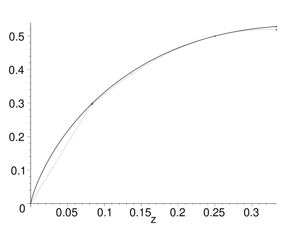
Figure 1: By virture of Shannon entropy function being lower-bounded by the polynomial functions, we can evaluate the von Neumann entropy of $\Xi$.

The first inequality of (17) is easily confirmed. On the other hand, one way of the proof of the second inequality is as follows: Let $f(z):=\bigl{(}-z\log_{2}z\bigr{)}-\left(\frac{1}{2}+\frac{\log_{e}4-1}{\log_{e}2}(z-\frac{1}{4})-4(z-\frac{1}{4})^{2}\right)$. Differentiating this expression by $z$ once and twice, we can get the increasing and decreasing table as follows.

$z$	$\frac{1}{12}$		$\frac{1}{8\log_{e}2}$		$\frac{1}{4}$		$\frac{1}{3}$
$f(z)$	$+$	$\curvearrowright$	$+$	$\searrow$	$0$	$\nearrow$
$f^{\prime}(z)$				$-$	$0$	$+$
$f^{\prime\prime}(z)$		$-$	$0$	$+$	$+$	$+$

The table indicates $f(z)\geq 0$ for $z\in\left[\frac{1}{12},\frac{1}{3}\right]$. Now we indeed get the lower bounds by polynomial functions.

Combining all of the above inequalities we get (16) as

$$-\sum\limits_{i=1}^{3}\lambda_{i}\log_{2}\lambda_{i}\geq 1+\left(\frac{\log_{e}3+2}{\log_{e}2}-2\right)\lambda_{1}+4\lambda_{1}^{2}\geq 1\quad.$$

so that (15) and (14) are successively shown and that our proof is finished. ∎

References

- [1] G. Vidal, W. Dür, J. I. Cirac, Entanglement Cost of Bipartite Mixed States (2002), Physical Review Letters, 89, 027901.
- [2] Peter W. Shor (2002), Additivity of the Classical Capacity of Entanglement-Breaking Quantum Channels, quant-ph/0201149.
- [3] K. Matsumoto, A. Winter, T. Shimono (2002), Remarks on additivity of the Holevo channel capacity and of the entanglement of formation, quant-ph/0206148.
- [4] Christopher King, Additivity for unital qubit channels (2001), quant-ph/0103156.
- [5] W. F. Stinespring (1955), Positive functions on –algebras, Proceedings of the American Mathematical Society, 6, 211-216.