Quantum Dissipation Induced
Noncommutative Geometry

Abstract

The quantum statistical dynamics of a position coordinate x coupled to a reservoir requires theoretically two copies of the position coordinate within the reduced density matrix description. One coordinate moves forward in time while the other coordinate moves backward in time. It is shown that quantum dissipation induces, in the plane of the forward and backward motions, a noncommutative geometry. The noncommutative geometric plane is a consequence of a quantum dissipation induced phase interference which is closely analogous to the Aharanov-Bohm effect.

PACS: 02.40.Gh, 11.10.Ef   –   Key words: noncommutative geometry, gauge theories, dissipation

1 Introduction

There has been considerable recent interest in the role of noncommutative geometry in quantum mechanics. The algebraic structures arising in that context have been analyzed[1]-[10]. In his work on the energy levels of a charged particle in a magnetic field, Landau pointed out the non-commuting nature of the coordinates of the center of the circular cyclotron trajectory[11]. The harmonic oscillator on the noncommutative plane, the motion of a particle in an external magnetic field and the Landau problem on the noncommutative sphere are only few examples of systems which have been studied in detail. Furthermore, noncommutative geometries are also of interest in Cern-Simons gauge theories, the usual gauge theories and string theories[12] -[17]. Non-zero Poisson brackets for the plane coordinates have been found in the study of the symplectic structure for a dissipative system in the case of strong damping $R\gg M$, i.e. the so-called reduced case[18]. The relation between dissipation and noncommutative geometry was also noticed[10] with reference to the reduced dissipative systems. The purpose of the present paper is twofold: (i) we show that quantum dissipation introduces its own noncommutative geometry and (ii) we prove that the quantum interference phase between two alternative paths in the plane (as in the Aharanov-Bohm effect) is simply determined by the noncommutative length scale and the enclosed area between the paths. This in turn provides the connection between the noncommutative length scale and the zero point fluctuations in the coordinates. The links we establish between noncommutative geometry, quantum dissipation, geometric phases and zero point fluctuations, may open interesting perspectives in many sectors of quantum physics, e.g. in quantum optics and in quantum computing or whenever quantum dissipation cannot be actually neglected in any reasonable approximation. They may also play a role in the ’t Hooft proposal[19] of the interplay between classical deterministic systems with loss of information and quantum dynamics in view of the established relation in that frame between geometric phase and zero point energy[20].

Perhaps the clearest example of a noncommutive geometry is the “plane”. Suppose that $(X,Y)$ represents the coordinates of a “point” in such a plane and further suppose that the coordinates do not commute; i.e.

$$\left[X,Y\right]=iL^{2},$$ (1)

where $L$ is the geometric length scale in the noncommutative plane. The physical meaning of $L$ becomes evident upon placing

$$Z=\frac{X+iY}{L\sqrt{2}},\ \ Z^{*}=\frac{X-iY}{L\sqrt{2}},$$ (2)

and

$$\left[Z,Z^{*}\right]=1,$$ (3)

into the noncommutative Pythagoras’ definition of distance $S$; It is

$$S^{2}=X^{2}+Y^{2}=L^{2}(2Z^{*}Z+1).$$ (4)

From the known properties of the oscillator destruction $Z$ and creation $Z^{*}$ operators in Eqs.(3) and (4), it follows that the Pythagorean distance is quantized in units of the length scale $L$ according to

$$S_{n}^{2}=L^{2}(2n+1)\ \ {\rm where}\ \ n=0,1,2,3,\ldots\ .$$ (5)

A quantum interference phase of the Aharanov-Bohm type can always be associated with the noncommutative plane. From a path integral quantum mechanical viewpoint, suppose that a particle can move from an initial point in the plane to a final point in the plane via one of two paths, say ${\cal P}_{1}$ or ${\cal P}_{2}$. Since the paths start and finish at the same point, if one transverses the first path in a forward direction and the second path in a backward direction, then the resulting closed path encloses an area ${\cal A}$. The phase interference between these two points is determined by the difference between the actions for these two paths $\hbar\vartheta={\cal S}({\cal P}_{1})-{\cal S}({\cal P}_{2})$. It will be shown in Sec.2 that the interference phase may be written as

$$\vartheta=\frac{\cal A}{L^{2}}.$$ (6)

A physical realization of the mathematical noncommutative plane is present in every laboratory wherein a charged particle moves in a plane with a normal uniform magnetic field ${\bf B}$. The nature of the noncommutative geometry and the Aharanov-Bohm effect which follows from the more general Eq.(6) will be discussed in Sec.3. For this case, there are two canonical pairs of position coordinates which do not commute; Namely, (i) the position ${\bf R}$ of the center of the cyclotron circular orbit and (ii) the radius vector ${\bf\rho}$ from the center of the circle to the charged particle position ${\bf r}={\bf R}+{\bf\rho}$. This is shown in Fig.1. The magnetic length scale of the noncommuting geometric coordinates is due to Landau,

$$L^{2}=\frac{\hbar c}{eB}=\frac{\phi_{0}}{2\pi B}\ \ \ {\rm(magnetic)},$$ (7)

where $\phi_{0}$ is the magnitude of the magnetic flux quantum associated with a charge $e$.

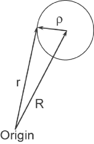
Figure 1: Shown is a charge $e$ moving in a circular cyclotron orbit. A noncommuting coordinate pair is ${\bf R}=(X,Y)$ which points from the origin to the orbit center. Another noncommuting coordinate pair is ${\bf\rho}=(\rho_{x},\rho_{y})$ which points from the center of the orbit to the charge position ${\bf r}={\bf R}+{\bf\rho}$.

Our main purpose here is to show that quantum dissipation introduces its own noncommutative geometry. The dissipative noncommutative plane consists of coordinates $(x_{+},x_{-})$ wherein $x_{+}$ denotes the coordinate $x$ moving forward in time and $x_{-}$ denotes the coordinate $x$ moving backward in time. The need for “two copies” $(x_{+},x_{-})$ for one physical coordinate $x$ is a consequence of employing a reduced density matrix $\left(x_{+}\left|\rho(t)\right|x_{-}\right)$ for describing quantum mechanical probabilities [21]-[24].

The reader is asked to consider a particle moving in a potential $U(x)$ under the further action of a linear force of friction. Classically, the equation of motion would be

$$M\frac{d^{2}x}{dt^{2}}+R\frac{dx}{dt}+U^{\prime}(x)=0.$$ (8)

In the “two coordinate” quantum mechanical version, Eq.(8) reads

$$M\frac{d^{2}x_{+}}{dt^{2}}+R\frac{dx_{-}}{dt}+U^{\prime}(x_{+}) = 0,$$

$$M\frac{d^{2}x_{-}}{dt^{2}}+R\frac{dx_{+}}{dt}+U^{\prime}(x_{-}) = 0.$$ (9)

The dissipative system will behave classically, as in Eq.(8), if and only if the forward and backward paths are nearly equal $x_{+}(t)\approx x_{-}(t)\approx x(t)$. On the other hand, if $x_{+}(t)$ is appreciably different from $x_{-}(t)$, then quantum interference will occur albeit in the presence of quantum dissipation [24]. It is remarkable the quantum interference can in fact be induced by dissipation. The derivation of Eqs.(9) will be discussed in Sec.4.

In Sec.5, the noncommuting position coordinates are introduced in the $(x_{+},x_{-})$ plane. The dissipation induced length scale $L$ is determined by

$$L^{2}=\frac{\hbar}{R}\ \ \ {\rm(dissipative)}.$$ (10)

Attention will then be paid to the situation in which the potential $U=0$ so that the force on the particle is purely that of friction. The situation is then closely analogous to the charged particle in an electric field since the cyclotron circular orbits here appear as Minkowski metric hyperbolic orbits. In the concluding Sec.6, the general physical basis for the quantum dissipation induced noncommuting geometry will be discussed.

2 Path Integrals and the Interference Phase

For motion at fixed energy one may (in classical mechanics) associate with each path ${\cal P}$ (in phase space) a phase space action integral

$${\cal S}({\cal P})=\int_{\cal P}p_{i}dq^{i}.$$ (11)

From the viewpoint of the path integral formulation of quantum mechanics one may consider many possible paths with the same initial point and final point. Let us concentrate on just two such paths ${\cal P}_{1}$ and ${\cal P}_{2}$. The phase interference $\vartheta$ between the two paths is determined by the action difference

$$\hbar\vartheta=\int_{{\cal P}_{1}}p_{i}dq^{i}-\int_{{\cal P}_{2}}p_{i}dq^{i}=\oint_{{\cal P}=\partial\Omega}p_{i}dq^{i}$$ (12)

wherein ${\cal P}$ is the closed path which goes from the initial point to the final point via path ${\cal P}_{1}$ and returns back to the initial point via ${\cal P}_{2}$. The closed ${\cal P}$ path may be regarded as the boundary of a two-dimensional surface $\Omega$; i.e. ${\cal P}=\partial\Omega$. Employing Stokes theorem in Eq.(12) yields

$$\vartheta=\frac{1}{\hbar}\oint_{{\cal P}=\partial\Omega}p_{i}dq^{i}=\frac{1}{\hbar}\int_{\Omega}(dp_{i}\wedge dq^{i}).$$ (13)

The quantum phase interference $\vartheta$ between two alternative paths is thereby proportional to an “area” of a surface $\Omega$ in phase space $(p_{1},\ldots,p_{f};q^{1},\ldots,q^{f})$ as described by the right hand side of Eq.(13).

If one briefly reverts to the operator formalism and writes the commutation Eq.(1) in the noncommutative plane as

$$[X,P_{X}]=i\hbar\ \ \ {\rm where}\ \ \ P_{X}=\left(\frac{\hbar Y}{L^{2}}\right),$$ (14)

then back in the path integral formalism Eq.(13) reads

$$\vartheta=\frac{1}{\hbar}\int_{\Omega}(dP_{X}\wedge dX)=\frac{1}{L^{2}}\int_{\Omega}(dY\wedge dX)$$ (15)

and we have proved the following:

Theorem: The quantum interference phase between two alternative paths in the plane is determined by the noncommutative length scale $L$ and the enclosed area ${\cal A}$ via

$$\vartheta=\frac{\cal A}{L^{2}}\ .$$ (16)

The existence of an interference phase is intimately connected to the zero point fluctuations in the coordinates; e.g. Eq.(1) implies a zero point uncertainty relation $\Delta X\Delta Y\geq(L^{2}/2)$.

3 Charged Particle in a Magnetic Field

Consider the motion of a non-relativistic charged particle in a plane perpendicular to a uniform magnetic field ${\bf B}$. The Hamiltonian is

$$H=\frac{1}{2M}\left({\bf p}-\frac{e}{c}{\bf A}\right)^{2}\ \ {\rm where}\ \ {\bf A}=(A_{x},A_{y})=\left(-\frac{By}{2},\frac{Bx}{2}\right).$$ (17)

Putting

$$\hbar{\bf K}={\bf p}-\frac{e}{c}{\bf A}=-i\hbar{\bf\nabla}-\frac{e}{c}{\bf A},$$ (18)

yields the equal time commutator

$$\left[K_{x},K_{y}\right]=\frac{ieB}{\hbar c}=\frac{i}{L^{2}}.$$ (19)

Let us now define the cyclotron radius vector ${\bf\rho}=(\rho_{x},\rho_{y})$ as

$$\rho_{x}=-L^{2}K_{y}\ \ {\rm and}\ \ \rho_{y}=L^{2}K_{x}.$$ (20)

If $M{\bf v}=\hbar{\bf K}$ were classical, then ${\bf\rho}$ would be the radius vector from the center of the circular cyclotron orbit to the position of the charge. When quantum mechanics is employed, the notion of a cyclotron orbit becomes blurred because the vector cyclotron radius has components which are noncommutative,

$$\left[\rho_{x},\rho_{y}\right]=iL^{2}.$$ (21)

The energy of the charged particle may still be written in terms of the cyclotron radius ${\bf\rho}$ and the cyclotron frequency $\omega_{c}$ as

$$H=\frac{1}{2}M\omega_{c}^{2}\rho^{2}=\frac{1}{2}M\omega_{c}^{2}(\rho_{x}^{2}+\rho_{y}^{2})\ \ {\rm where}\ \ \omega_{c}=\frac{eB}{Mc}\ .$$ (22)

The noncommutative geometrical Pythagorean theorem yields the quantized radius vector values

$$\rho_{n}^{2}=L^{2}(2n+1)\ \ \ \ (n=0,1,2,3,\ldots).$$ (23)

Eqs.(22) and (23) imply the Landau magnetic energy spectrum

$$E_{n}=\hbar\omega_{c}\left(n+\frac{1}{2}\right)\ \ \ \ (n=0,1,2,3,\ldots).$$ (24)

Note that the position of the charge ${\bf r}=(x,y)$ has components which commute $[x,y]=0$, but these do not commute with the cyclotron radius components; i.e. we have from Eqs.(18) and (20) that

$$\left[\rho_{x},x\right] = \left[\rho_{y},y\right]\ =\ 0,$$

$$\left[\rho_{x},y\right] = \left[x,\rho_{y}\right]\ =\ iL^{2}.$$ (25)

We then introduce the coordinate ${\bf R}=(X,Y)$ as the center of the cyclotron orbit via

$${\bf r}={\bf R}+{\bf\rho}$$ (26)

and find that

$$\left[X,Y\right]=-iL^{2}.$$ (27)

Thus ${\bf R}=(X,Y)$ and ${\bf\rho}=(\rho_{x},\rho_{y})$ represent two independent pairs of geometric canonical conjugate variables; i.e $[R_{i},\rho_{j}]=0$.

From a path integral viewpoint, the quantum interference phase in the plane is described by Eq.(16). For the magnetic field problem the theorem reads

$$\vartheta=\frac{\cal A}{L^{2}}=\frac{\cal A}{\hbar c/eB}=\frac{e\Phi}{\hbar c},$$ (28)

where $\Phi=B{\cal A}$ is the magnetic flux through the enclosed area ${\cal A}$. Eq.(28) represents precisely the Aharanov-Bohm effect.

Finally, in the operator (as opposed to path integral) version of quantum mechanics, the area enclosed by the cyclotron orbit in the plane has the discrete spectrum

$${\cal A}_{n}=\pi\rho_{n}^{2}=\pi L^{2}(2n+1)=\frac{2\pi\hbar c}{eB}\left(n+\frac{1}{2}\right).$$ (29)

This means that as the radii of the cyclotron increase, the added magnetic flux comes in units of the flux quantum $\phi_{0}$; i.e.

$$\Delta\Phi=B({\cal A}_{n+1}-{\cal A}_{n})=\frac{2\pi\hbar c}{e}=\phi_{0}.$$ (30)

Such magnetic flux quantization here arises as a consequence of the area quantization which is intrinsic to the noncommutative plane.

4 Quantum Friction

The quantum properties of a “position coordinate” $x$ of a particle are best described by making “two copies” of the coordinate $x\to(x_{+},x_{-})$ [21]-[24]. For computing averages of any possible associated operator (say $Q$) employing a reduced density matrix (say $\rho$) one must integrate over both coordinates ($x_{+}$ and $x_{-}$) in the copies; i.e. the averaged value of $Q$ is of the form

$$\left<Q\right>=Tr\left(\rho Q\right)=\int\int\left(x_{+}\left|\rho\right|x_{-}\right)\left(x_{-}\left|Q\right|x_{+}\right)dx_{+}dx_{-}.$$ (31)

For a particle moving in one dimension with a Hamiltonian

$$H=\frac{p^{2}}{2M}+U(x)=-\frac{\hbar^{2}}{2M}\left(\frac{\partial}{\partial x}\right)^{2}+U(x),$$ (32)

the time dependence,

$$\rho(t)=e^{-iHt/\hbar}\rho e^{iHt/\hbar},$$ (33)

reads (in the coordinate representation)

$$\left(x_{+}\left|\rho(t)\right|x_{-}\right)=e^{-i(H_{+}-H_{-})t/\hbar}\left(x_{+}\left|\rho\right|x_{-}\right),$$ (34)

where the two copies of the Hamiltonian

$$H_{\pm}=\frac{p_{\pm}^{2}}{2M}+U(x_{\pm})=-\frac{\hbar^{2}}{2M}\left(\frac{\partial}{\partial x_{\pm}}\right)^{2}+U(x_{\pm})$$ (35)

drive $x_{+}$ forward in time and drive $x_{-}$ backward in time. The equation of motion for the density matrix is then

$$i\hbar\frac{\partial}{\partial t}\left(x_{+}\left|\rho(t)\right|x_{-}\right)={\cal H}_{0}\left(x_{+}\left|\rho(t)\right|x_{-}\right)$$ (36)

wherein

$${\cal H}_{0}=H_{+}-H_{-}=\frac{p_{+}^{2}}{2M}+U(x_{+})-\frac{p_{-}^{2}}{2M}-U(x_{-}).$$ (37)

The notion of quantum dissipation enters into our considerations if there is a coupling to a thermal reservoir yielding a mechanical resistance $R$. The full equation of motion has the form

$$i\hbar\frac{\partial}{\partial t}\left(x_{+}\left|\rho(t)\right|x_{-}\right)={\cal H}\left(x_{+}\left|\rho(t)\right|x_{-}\right)-\left(x_{+}\left|N[\rho]\right|x_{-}\right),$$ (38)

where $N[\rho]\approx(ik_{B}TR/\hbar)[x,[x,\rho]]$ describes the effects of the reservoir random thermal noise and the new “Hamiltonian” ${\cal H}_{0}\to{\cal H}$ for motion in the $(x_{+},x_{-})$ plane has been previously discussed[23, 24]

$${\cal H}=\frac{1}{2M}\left\{\left(p_{+}-\frac{Rx_{-}}{2}\right)^{2}-\left(p_{-}+\frac{Rx_{+}}{2}\right)^{2}\right\}+U(x_{+})-U(x_{-}).$$ (39)

The velocity components $(v_{+},v_{-})$ in the $(x_{+},x_{-})$ plane may be found from the Hamiltonian equation

$$v_{\pm}=\dot{x}_{\pm}=\frac{\partial{\cal H}}{\partial p_{\pm}}=\pm\frac{1}{M}\left(p_{\pm}\mp\frac{Rx_{\mp}}{2}\right).$$ (40)

Similarly,

$$\dot{p}_{\pm}=-\frac{\partial{\cal H}}{\partial x_{\pm}}=\mp U^{\prime}(x_{\pm})\mp\frac{Rv_{\mp}}{2}\ .$$ (41)

From Eqs.(40) and (41) it follows that

$$M\dot{v}_{\pm}+Rv_{\mp}+U^{\prime}(x_{\pm})=0$$ (42)

in agreement with Eqs.(9). The classical equation of motion including dissipation thereby holds true if $x_{+}(t)\approx x_{-}(t)\approx x(t)$. Dissipation induced quantum interference takes place if and only if the forward in time paths differ appreciably from the backward in time paths[24].

5 Dissipative Noncommutative Plane

The commutation relations in the dissipative $(x_{+},x_{-})$ plane may now be derived. If we define

$$Mv_{\pm}=\hbar K_{\pm},$$ (43)

then one finds from Eq.(40) that

$$\left[K_{+},K_{-}\right]=\frac{iR}{\hbar}=\frac{i}{L^{2}}\ .$$ (44)

A canonical set of conjugate position coordinates $(\xi_{+},\xi_{-})$ may be defined by

$$\xi_{\pm} = \mp L^{2}K_{\mp}$$

$$\left[\xi_{+},\xi_{-}\right] = iL^{2}.$$ (45)

Another canonical set of conjugate position coordinates $(X_{+},X_{-})$ may be defined by

$$x_{+}=X_{+}+\xi_{+} x_{-}=X_{-}+\xi_{-}$$ ,

$$\left[X_{+},X_{-}\right] = -iL^{2}.$$ (46)

Note that $[X_{a},\xi_{b}]=0$ , where $a=\pm$ and $b=\pm$.

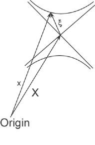
Figure 2: Shown is the hyperbolic path of a particle moving in the $x=(x_{+},x_{-})$ plane. A noncommuting coordinate pair is $X=(X_{+},X_{-})$ which points from the origin to hyperbolic center. Another noncommuting coordinate pair is $\xi=(\xi_{+},\xi_{-})$ which points from the center of the orbit to the position on the hyperbola. $x=X+\xi$.

For the case of pure friction in which the potential $U=0$, Eqs.(39), (43) and (45) imply

$${\cal H}_{friction}=\frac{\hbar^{2}}{2M}(K_{+}^{2}-K_{-}^{2})=-\frac{\hbar^{2}}{2ML^{4}}(\xi_{+}^{2}-\xi_{-}^{2}).$$ (47)

The equations of motion read

$$\dot{\xi}_{\pm}=\frac{i}{\hbar}\left[{\cal H}_{friction},\xi_{\pm}\right]=-\frac{\hbar}{ML^{2}}\xi_{\mp}=-\frac{R}{M}\xi_{\mp}=-\Gamma\xi_{\mp},$$ (48)

with the solution

$$\left(\begin{array}[]{c}\xi_{+}(t)\\ \xi_{-}(t)\\ \end{array}\right)=\left(\begin{array}[]{cc}\cosh(\Gamma t)&-\sinh(\Gamma t)\\ -\sinh(\Gamma t)&\cosh(\Gamma t)\\ \end{array}\right)\left(\begin{array}[]{c}\xi_{+}\\ \xi_{-}\\ \end{array}\right).$$ (49)

Eq.(49) describes the hyperbolic orbit

$$\xi_{-}(t)^{2}-\xi_{+}(t)^{2}=\frac{2L^{2}{\cal{H}}_{friction}}{\hbar\Gamma}\ .$$ (50)

A comparison can be made between the noncommutative dissipative plane and the noncommutative Landau magnetic plane as shown in Fig.2. The circular orbit in Fig.1 for the magnetic problem is here replaced by the hyperbolic orbit. In view of the minus sign in the “kinetic” energy,

$${\cal H}_{friction}=\frac{M}{2}(v_{+}^{2}-v_{-}^{2}),$$ (51)

it is best to view the metric as pseudo-Euclidean or equivalently we can use the Minkowski metric $u\cdot w=u_{+}w_{+}-u_{-}w_{-}$ .

In fact, the quantum dissipative eigenvalue problem ${\cal H}_{friction}\ \tilde{\rho}_{\omega}=\hbar\omega\tilde{\rho}_{\omega}$ is formally identical to the relativistic charged scalar field equation in $(1+1)$ dimensional quantum electrodynamics; i.e.

$$\left\{-d_{\mu}d^{\mu}+\left(\frac{mc}{\hbar}\right)^{2}\right\}\psi(x)=0,$$

$$K_{\mu}=-id_{\mu}=-i\partial_{\mu}+\frac{eA_{\mu}}{\hbar c},$$

$$\left[K_{\mu},K_{\nu}\right]=\frac{i\hbar eF_{\mu\nu}}{c}\ .$$ (52)

Since in $(1+1)$ dimensional electrodynamics, the only nonzero tensor components describe the electric field $F_{10}=-F_{01}=E$, it follows by comparing Eqs.(44) and (52) that the analogy is exact if $L^{2}=(\hbar/R)=(\hbar c/eE)$. Note that the interference phase is thereby

$$\vartheta = \frac{e\Phi}{\hbar c}=\frac{e}{\hbar c}\oint_{{\cal P}\partial\Omega}A_{\nu}dx^{\nu}$$ (53)

$$= \frac{e}{2\hbar c}\int_{\Omega}F_{\mu\nu}dx^{\mu}\wedge dx^{\nu}$$

$$= \frac{eE{\cal A}}{\hbar c}=\frac{\cal A}{L^{2}}\ .$$

Thus, the Minkowski metric implies a closer analogy with the electric flux than with the magnetic flux. The hyperbolic orbit in Fig.2 is reflected in the classical orbit for a charged particle moving along the $x$-axis in a uniform electric field. The hyperbolae are defined by $(x-X)^{2}-c^{2}(t-T)=\Lambda^{2},$ where $\Lambda^{2}=(mc^{2}/eE)^{2}=(mc/\hbar L^{2})^{2}$, the hyperbolic center is at $(X,cT)$ and one branch of the hyperbolae is a charged particle moving forward in time while the other branch is the same particle moving backward in time as an anti-particle.

6 Remarks and Conclusions

We have discussed above the dissipative quantum statistical dynamics of a coordinate $x$ coupled to a reservoir yielding friction effects. The reduced density matrix description requires theoretically two copies of the position coordinate $(x_{+},x_{-})$ with $x_{+}$ moving forward and $x_{-}$ moving backward in time. Both decay $\exp(-\Gamma t)$ and amplification $\exp(\Gamma t)$ enter into the motions of $x_{\pm}(t)$. Quasi-classically, the motions proceed on two branches of hyperbolae whose center $X=(X_{+},X_{-})$ and relative displacements $\xi=(\xi_{+},\xi_{-})$ are independent canonical conjugate pairs which obey the rules of the non-commutative plane; i.e.

$$\left[\xi_{+},\xi_{-}\right] = iL^{2}$$

$$\left[X_{+},X_{-}\right] = -iL^{2}$$ (54)

The noncommutative geometric plane is intimately related to an interference phase which can serve as a quantum basis for deriving the canonical commutation relations between coordinates in the plane. For completeness of presentation we derive in the appendix to this work the noncommuting geometry vortex coordinates[25] in thin superfluid films possibly induced by rotations of the superfluid container or substrate[26].

For the problem at hand, a density matrix equation of motion $i\hbar\dot{\rho}={\cal H}\rho$ leads to an eigenvalue problem ${\cal H}\rho_{\omega}=\hbar\omega\rho_{\omega}$ which directly yields the quantum frequency spectrum. If the system were isolated, then ${\cal H}=H_{+}-H_{-}$. For isolated quantum systems, the frequencies can be identified with the Bohr transition frequencies $\omega_{fi}=E_{f}-E_{i}$. Thus a quantum jump $i\to f$ involves a transition from a backward in time motion to a forward in time motion as is evident from $\exp(-i\omega_{fi}t)=\exp(-iE_{f}t/\hbar)\exp(iE_{i}t/\hbar).$

If the quantum system is not isolated, then the forward in time to the backward in time transitions are strongly coupled. Nevertheless the eigenvalue problem

$${\cal H}\rho_{\omega}=\hbar\omega\rho_{\omega}$$ (55)

still describes the quantum spectroscopic frequency spectrum. For the problem of pure frictional damping, we have from Eqs.(45) and (47) that

$${\cal H}_{friction}=\frac{\Pi_{+}^{2}}{2M}-\frac{M\Gamma^{2}}{2}\xi_{+}^{2},\ \ {\rm where}\ \ {\Pi}_{+}=\frac{\hbar\xi_{-}}{L^{2}}\ .$$ (56)

Since $[\Pi_{+},\xi_{+}]=-i\hbar$ the operator Eq.(56) represents an “inverted oscillator”. The barrier transmission coefficient $P(\omega)$ for the inverted oscillator is well known[11]; It is

$$P(\omega)=\frac{1}{1+e^{-2\pi\omega/\Gamma}}\ .$$ (57)

Thus there is a possibility of jumping from the forward direction in time to the backward direction of time or vice versa. Such quantum jumps are required for the Bohr frequencies $\omega$ in an open (dissipative) system.

We observe that our conclusions may be extended to the three-dimensional topological massive Chern-Simons gauge theory in the infrared limit and to the Bloch electron in a solid. We recall indeed that the Lagrangian for the system of Eqs.(9) has been found [18] to be the same as the Lagrangian for three-dimensional topological massive Chern-Simons gauge theory in the infrared limit. It is also the same as for a Bloch electron in a solid which propagates along a lattice plane with a hyperbolic energy surface[18]. In the Chern-Simons case we have $\theta_{CS}=R/M=(\hbar/ML^{2})$, with $\theta_{CS}$ the “topological mass parameter”. In the Bloch electron case, $(eB/\hbar c)=(1/L^{2})$, with $B$ denoting the $z$-component of the applied external magnetic field. In ref. [18] (see also [10]) it has been considered the symplectic structure for the system of Eqs. (9) in the case of strong damping $R\gg M$ (the so-called reduced case) in the Dirac constraint formalism as well as in the Faddeev and Jackiw formalism [27] and in both formalisms a non-zero Poisson bracket for the ($x_{+},~{}x_{-}$) coordinates has been found.

Acknowledgements

The authors would like to thank INFN, INFM and ESF Program COSLAB for partial support of this work.

APPENDIX

In thin superfluid $He^{4}$ films on solid substrates, vortices can exist. The coordinates (x,y) locating the core of a single vortex do not commute with each other and thus determine a noncommutative geometry. Let us see how this comes about.

The superfluid velocity field ${\bf v}_{s}$ rotating around the vortex core is related to the phase of the wave function via

$${\bf v}_{s}={\hbar\over m}{\bf grad}\ (\sigma\theta),$$

where $\sigma=\pm 1$ depending on the orientation of the vortex. For such a flow, the many body wave function has the form

$$\Psi\approx\exp\big{(}i\sigma\sum_{j}\theta({\bf r}_{j})\big{)}\Psi_{0}$$

wherein $\Psi_{0}$ is real. Because $\theta$ is a phase, we have for an integral around the core

$$\oint_{(around\ core)}d\theta=2\pi.$$

Thus one has the circulation quantization

$$m\oint_{(around\ core)}{\bf v}_{s}\cdot d{\bf r}=2\pi\sigma\hbar\ \ {\rm where}\ \ {(\sigma=\pm 1)}.$$

Now let us consider what happens if we move the core around a closed path ${\cal P}=\partial\Omega$ wherein the enclosed area contains ${\cal N}(\Omega)$ adsorbed atoms. Each atom whose position obeys ${\bf r}_{j}\in\Omega$ receives a change of $2\pi\sigma$ in the total phase. Each atom which obeys ${\bf r}_{j}\notin\Omega$ receives no phase change. Thus the total phase change which takes place as the core is brought around a closed path is given by

$$\vartheta=2\pi\sigma{\cal N}(\Omega).$$

If $n={\cal N}(\Omega)/{\cal A}(\Omega)$ denotes the number of atoms per unit area adsorbed on the film, then

$$\vartheta=2\pi\sigma{\cal N}=2\pi\sigma n{\cal A}.$$

Comparing the above equation with our central theorem Eq.(16), we find that $L^{2}=(2\pi n)^{-1}$ and that the position of the vortex cores on the substrate obey

$$\left[x,y\right]=\left(\frac{i}{2\pi n}\right)\sigma\ \ {\rm where}\ \ {(\sigma=\pm 1)}.$$

The noncommutative geometry length scale $L$ is of the order of the vortex core size.

References

- [1] V. P. Nair and A. P. Polychronakos, Phys. Lett. B 505, 267 (2001)
- [2] Z. Guralnik, R. Jackiw, S. Y. Pi and A. P. Polychronakos, Phys. Lett. B 517, 450 (2001)
- [3] S. Bellucci and A. Nersessian, Phys. Lett. B 542, 295 (2002)
- [4] S. Bellucci, A. Nersessian and C. Sochichiu, Phys. Lett. B 522, 345 (2001)
- [5] J. Lukierski, P. C. Stichel and W. J. Zakrzewski, Annals Phys. 260, 224 (1997)
- [6] C. Duval and P. A. Horvathy, Phys. Lett. B 479, 284 (2000)
- [7] Y. N. Srivastava and A. Widom, arXiv:hep-ph/0109020
- [8] A. Widom and Y. N. Srivastava, arXiv:hep-ph/0111350
- [9] P. Castorina, A.Iorio and D. Zappalà, Noncommutative synchrotron, MIT-CPT 3336
- [10] R. Banerjee, arXiv:hep-th/0106280
- [11] L.D.Landau and E.M.Lifshitz, Quantum Mechanics, Pergamon Press, Oxford 1977, pp.458 and 184
- [12] G. V. Dunne, R. Jackiw and C. A. Trugenberger, Phys. Rev. D 41, 661 (1990)
- [13] R. Banerjee, arXiv:hep-th/0210259
- [14] A. Iorio and T. Sykora, Int. J. Mod. Phys. A 17, 2369 (2002)
- [15] A. Connes, M. R. Douglas and A. Schwarz, JHEP 9802, 003 (1998)
- [16] N. Seiberg and E. Witten, JHEP 9909, 032 (1999)
- [17] R. Banerjee and S. Ghosh, Phys. Lett. B 533 (2002) 162
- [18] M. Blasone, E. Graziano, O. K. Pashaev and G. Vitiello, Annals Phys. 252, 115 (1996)
-
[19]
G. ’t Hooft,
Class. Quant. Grav. 16, 3263 (1999)
G. ’t Hooft, in “Basics and Highlights of Fundamental Physics”, Erice, (1999) [hep-th/0003005]
G. ’t Hooft, J. Statist. Phys. 53, 323 (1988) -
[20]
M. Blasone, P. Jizba and G. Vitiello,
Phys. Lett. A 287 (2001) 205
M. Blasone, E. Celeghini, P. Jizba and G. Vitiello, arXiv:quant-ph/0208012 -
[21]
R.P.Feynman, Statistical
Mechanics: A set of Lectures,
W.A. Benjamin, Reading, MA 1972
R. P. Feynman and F. L. Vernon, Annals Phys. 24, 118 (1963)
J. Schwinger, J.Math. Phys. 2, 407 (1961) - [22] E. Celeghini, M. Rasetti and G. Vitiello, Annals Phys. 215, 156 (1992)
- [23] Y. N. Srivastava, G. Vitiello and A. Widom, Annals Phys. 238, 200 (1995)
- [24] M. Blasone, Y. N. Srivastava, G. Vitiello and A. Widom, Annals Phys. 267, 61 (1998)
- [25] L. Mittag, M. Stephen and W. Yourgrau, Variational Principles in Hydrodynamics in W. Yourgrau and S. Mandelstam, Variational Principles in Dynamics and Quantum Theory, W. B. Saunders Co., Philidelphia 1968
- [26] A. Widom, Phys. Rev. 168, 150 (1968)
- [27] L.D. Faddeev and R. Jackiw, Phys. Rev. Lett. 60, 1692 (1988)