Security of the Bennett 1992 quantum-key distribution against individual attack over a realistic channel

Abstract

The security of two-state quantum key distribution against individual attack is estimated when the channel has losses and noises. We assume that Alice and Bob use two nonorthogonal single-photon polarization states. To make our analysis simple, we propose a modified B92 protocol in which Alice and Bob make use of inconclusive results and Bob performs a kind of symmetrization of received states. Using this protocol, Alice and Bob can estimate Eve’s information gain as a function of a few parameters which reflect the imperfections of devices or Eve’s disturbance. In some parameter regions, Eve’s maximum information gain shows counter-intuitive behavior, namely, it decreases as the amount of disturbances increases. For a small noise rate Eve can extract perfect information in the case where the angle between Alice’s two states is small or large, while she cannot extract perfect information for intermediate angles. We also estimate the secret key gain which is the net growth of the secret key per one pulse. We show the region where the modified B92 protocol over a realistic channel is secure against individual attack.

I Introduction

Quantum key distribution (QKD) is a way to share between the sender, Alice, and the receiver, Bob, a secret key whose information is not known to the eavesdropper, Eve. Since the first QKD protocol, called BB84 protocol, was introduced by Bennett and Brassard BB84 , several schemes for QKD have been proposed, such as Ekert protocol ekert , which is based on the nonlocality of quantum mechanics, B92 protocol B92 , which uses two nonorthogonal states, and so on imoto . In each protocol, since Eve cannot eavesdrop without disturbing quantum states, she will induce some errors or changes in the transmission rate. In ideal situations where imperfections such as transmission losses and dark counting of detectors do not exist, one can prove that the QKD protocols are secure even when Eve employs any kind of eavesdropping strategies including so-called collective attack or coherent attack, which is the most general attack where a single probe is entangled to the whole transmitted pulses. In practice, however, imperfections exist and if Eve gets rid of imperfections by using her unlimited technology (for example, she may replace the noisy channel to a noiseless channel), Eve can disturb quantum states to a certain degree and therefore she obtains some information about the secret key. Estimation of the amount of information extracted by Eve and construction of a secure secret key under such situations are not a trivial problem.

There are several works which deal with the security of realistic QKD. In BB841 ; BB842 ; BB843 ; simple ; inamori , it is proven that under some conditions the BB84 protocol is secure even when Eve employs coherent attack. The security proof in simple reveals a tight connection to the entanglement purification protocol EPP and quantum error correcting codes, especially Calderbank-Shor-Steane codes CSS . This proof can be also applied to BB84-type protocols such as the 6-state protocol six where the basis information is exchanged over a public channel. The security against the individual attack, which is more restricted but more realistic, was also discussed for the BB84 protocol norbert2 and for the Ekert protocol waks .

On the other hand, we have not yet fully understood the security of the B92 protocol. The discussions so far concerned with the security against individual attack fuchs ; slu . In each paper, the single-photon polarization is used as a carrier of the quantum signals, and the transmission loss is not included. In fuchs , Fuchs and Peres have calculated the upper bound of Eve’s Shannon information gain averaged over all transmitted bits. Slutsky and co-authers have estimated the upper bound of Eve’s Renyi information gain in a B92 protocol as a function of the error rate when Alice and Bob discard errors slu . The B92 protocol, which uses only two states, is conceptually the simplest of all the protocols. In addition, the protocol includes a continuous parameter (the nonorthogonality between the two states) that can be chosen by the users, forming a striking contrast to the BB84-type protocols. Further understanding of the security of the B92 protocol is thus important not only for the practical applications but also for deeper understanding of the nature of quantum information.

In this paper, we estimate the security of the B92 protocol against individual attack over a realistic channel including noises and transmission losses. We assume, like in fuchs ; slu , that Alice encodes the bit values in two single-photon polarization states (the original B92 in B92 uses two nonorthogonal coherent states). We consider a modified protocol in which inconclusive measurement results are also used for the estimation of Eve’s information gain, in addition to the bit error rate used in the previous analyses. The problem is also regarded as one of the basic problems of quantum eavesdropping, namely, the maximum information leak to an adversary who are simulating the noisy quantum channel through which Alice transmits Bob a bit encoded on two quantum states.

We briefly describe how Alice and Bob can obtain the secret key whose information available to Eve is negligibly small. First, Alice prepares nonorthogonal single- photon polarization states $|\,0\,\rangle$ and $|\,1\,\rangle$, depending on the bit values of the raw key, and sends them to Bob. After propagating through the noisy channel or through eavesdropping by Eve, $|\,0\,\rangle$ and $|\,1\,\rangle$ generally become mixed states, $\rho_{0}$ and $\rho_{1}$, respectively. Secondly, Bob performs measurement whose outcomes are 0, 1 and “?”. The outcome “?” means an inconclusive result where Bob cannot determine which state Alice has sent. Thirdly, Alice and Bob discard inconclusive bits and they reconcile the errors in conclusive bits by an error correction protocol which is the technique of classical information theory to obtain the reconciled key. Finally, in order to eliminate Eve’s information about the reconciled key, Alice and Bob shorten their keys via a privacy amplification protocol privacy amp , which is also the technique of the classical information theory. How much they should shorten the reconciled key depends on how much information about the reconciled key Eve could have obtained. The last two procedures are done over a public channel. It is assumed that Eve can listen to the information exchanged over the public channel, but she cannot alter it. By means of these techniques, Alice and Bob can obtain the identical secret key, even under the imperfections and Eve’s interference.

In the above framework, it is important for Alice and Bob to estimate Eve’s information about the reconciled key properly. To estimate this information, we propose a slightly modified protocol. The difference between our protocol and the original protocol is that when Bob obtains an inconclusive result, Alice opens which state she has sent. Using this extra data, Bob performs data processing which is a kind of symmetrization of the states received by Bob. This makes our analysis simpler without underestimating Eve’s ability. We can estimate Eve’s information by using the symmetrized density matrices. Eve’s information gain is calculated as a function of a few parameters which characterize the symmetrized density matrices. Since Bob’s symmetrized density matrices can be fully characterized by the observed quantities and classical communication, the problem we have solved is equivalent to the problem of how much maximum information Eve can extract while she simulates the noisy channel. The answer to this problem has turned out to be more complex than expected; We found a counter-intuitive phenomenon where the maximum information gain is not monotone increasing as a function of the amount of noises when the angle between Alice’s two states is small. We also found that for a small noise rate, Eve can extract perfect information in the case where the angle of Alice’s two states is very small or very large, while she cannot extract perfect information for the intermediate angle. We give an explanation that is useful to understand these behavior intuitively.

We also performed an optimization of the angle between Alice’s two states that makes the rate of the final key gain as high as possible. We show that the optimized angle decreases as the amount of noises and the transmission losses increase. Unfortunately, the assumption of the polarization encoding makes the B92 protocol particularly weak against channel losses, so that the key gain is always smaller than in the BB84 protocol.

This paper is organized as follows. In Sec. II, we describe our assumption on the apparatus used by Alice and Bob, and the limitation on Eve’s strategy. Our slightly modified B92 protocol is proposed in Sec. III. Then, in Sec. IV, we consider Bob’s data processing for the symmetrization of the density matrices, and in Sec. V, we optimize Eve’s eavesdropping strategy and calculate Eve’s maximum information gain as a function of the parameters that reflect imperfections or Eve’s disturbance. In Sec. VI, we calculate the secret key gain as a function of these parameters. Finally Sec. VII is devoted to the summary and discussion.

II Assumptions

In this section, we describe the assumptions on the abilities of the legitimate users (Alice and Bob) and the eavesdropper (Eve). We put these conditions throughout this paper.

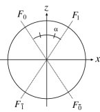
First, we describe what Alice and Bob perform with ideal apparatus. The B92 protocol is originally considered to use two nonorthogonal coherent states. In this paper, however, we assume two nonorthogonal single-photon polarization states for the simplicity of analysis. We denote the Hilbert space for each pulse as $H$, which contains arbitrary photon number states, and the subspace that contains only one photon as $H_{1}$. The subspace $H_{1}$ is two-dimensional reflecting the polarization degree of freedom, and the states in $H_{1}$ are conveniently represented by the Bloch sphere. We define $|\,\sigma_{\varphi}\,\rangle$ and $|\,\overline{\sigma_{\varphi}}\,\rangle$ for $-\pi<\varphi<\pi$ as follows,

$$|\,\sigma_{\varphi}\,\rangle \equiv \cos\frac{\varphi}{2}|\,z+\,\rangle+\sin\frac{\varphi}{2}|\,z-\,\rangle,$$

$$|\,\overline{\sigma_{\varphi}}\,\rangle \equiv \sin\frac{\varphi}{2}|\,z+\,\rangle-\cos\frac{\varphi}{2}|\,z-\,\rangle\,\,{\rm for}\,\,\varphi\geq 0\,,$$

$${\rm and}\,|\,\overline{\sigma_{\varphi}}\,\rangle \equiv -\sin\frac{\varphi}{2}|\,z+\,\rangle+\cos\frac{\varphi}{2}|\,z-\,\rangle\,\,{\rm for}\,\,\varphi<0\,,$$ (1)

where $|\,z+\,\rangle$ and $|\,z-\,\rangle$ are the eigenstates of $\sigma_{z}$ ($z$ component of Pauli matrix) whose eigenvalues are $+1$ and $-1$, respectively. $\varphi$ is the angle between $|\sigma_{\varphi}\rangle$ and $|\,z+\,\rangle$ on the $x-z$ plane in the Bloch sphere.

We assume that Alice prepares the following states depending on the bit value,

$$|\,0\rangle\equiv|\,\sigma_{-\alpha^{\prime}}\rangle\,\,{\rm and}\,|\,1\rangle\equiv|\,\sigma_{\alpha^{\prime}}\,\rangle\quad(0\leq\alpha^{\prime}\leq\pi/2),$$ (2)

where the parameter $\alpha^{\prime}$ characterizes the nonorthogonality between the two states, such that

$$\langle 0|1\rangle=\cos\alpha^{\prime}\,.$$ (3)

When these states are sent to Bob through the noisy quantum channel, $|\,0\,\rangle$ and $|\,1\,\rangle$ generally become mixed states, $\rho_{0}$ and $\rho_{1}$, respectively. On these states, Bob measures the polarization on the basis $\{|\,\sigma_{-\alpha}\rangle,|\,\overline{\sigma_{-\alpha}}\rangle\}$ or $\{|\,\sigma_{\alpha}\rangle,|\,\overline{\sigma_{\alpha}}\rangle\}$, which is selected randomly. The whole measurement process is described by the following POVM sPOVM

$$F_{0} \equiv \frac{1}{2}\,|\,\sigma_{-\alpha}\rangle\langle\sigma_{-\alpha}|$$

$$F_{\overline{0}} \equiv \frac{1}{2}\,|\,\overline{\sigma_{-\alpha}}\rangle\langle\overline{\sigma_{-\alpha}}|$$

$$F_{1} \equiv \frac{1}{2}\,|\,\sigma_{\alpha}\rangle\langle\sigma_{\alpha}|$$

$$F_{\overline{1}} \equiv \frac{1}{2}\,|\,\overline{\sigma_{\alpha}}\rangle\langle\overline{\sigma_{\alpha}}|$$

$$F_{{\rm V}} \equiv 1-F_{0}-F_{\overline{0}}-F_{1}-F_{\overline{1}}$$ (4)

where “V” means the states which contain zero or more than one photon, where allowances are made for the effect of transmission losses. $F_{{i}}$ and $F_{\overline{i}}$ ($i=0,1$) are shown in Fig. 1 schematically using Bloch sphere. Here we allow general cases where $\alpha$ is not necessarily equal to $\alpha^{\prime}$. We call the events inconclusive where Bob’s outcome of the measurement is $0$ or $1$, and the events where Bob’s outcome is $\overline{0}$ or $\overline{1}$ conclusive.

Figure 1: Bob’s measurement basis in the Bloch sphere.

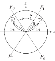
In reality, the transmission line and Alice and Bob’s apparatus is not perfect (see Fig. 2). We assume one condition on the character of the imperfection, namely, the imperfection is equivalently represented as a noise source placed just after Alice’s ideal apparatus, and a noise source just before Bob’s ideal apparatus. Under this condition, Fig. 2 becomes Fig. 3. We need some care for this assumption. For example, if the noisy photon detectors PD1 and PD2 in Fig. 2 have different quantum efficiencies, we cannot transform this model into Fig. 3 directly. However, if Bob interchanges noisy PD 1 and noisy PD 2 at random, which effectively makes the efficiency of these detectors identical, we can transform Fig. 2 into Fig. 3, and the assumption can be met.

The benefit of the above assumption is that we can use a simpler model in which Alice and Bob’s apparatus is perfect, in the following sense. In Fig. 3, the region bounded by dash-dotted lines is under Eve’s control. Suppose that this region is extended up to the dotted lines. While this assumption may make the length of the final key shorter than the optimum one, at least we can avoid the risk of underestimating Eve’s ability. In this model, every imperfection is attributed to the property of the quantum channel, and the analysis is considerably simplified. This assumption has been also used in the previous works waks ; esti .

Figure 2: An example of experimental setup. “noisy PR” is the noisy polarization rotator, “noisy PBS” is a noisy polarization beam splitter, and “noisy PD1” and “noisy PD2” are noisy photon detectors. Our assumption is that this setup can be transformed into Fig. 3.

Figure 3: The model of our setup. The “NS” represents the noise source of Alice or Bob’s device. Since Alice and Bob cannot separate noises due to imperfections and ones due to Eve, they should assume, for security, that Eve can also control NS, which extends Eve’s region up to dotted line. Due to this assumption, the legitimate users’ apparatuses look like ideal. “Ideal PR” is an ideal polarization rotator which accurately rotates the polarization of photons, “ideal PBS” is an ideal polarization beam splitter, and “ideal PD 1 (2)” is an ideal photon detector with unit quantum efficiency and no dark counting.

We assume that Eve’s eavesdropping is restricted to individual attack. The definition of individual attack is that eavesdropping is independently done for each pulse and there exists no correlation of events among pulses. In the most general individual attack, Eve prepares her auxiliary system (probe) E in an initial state $|w\rangle_{\rm E}$, interacts it with one pulse sent by Alice via a unitary operation $U$, and performs measurements on the probe E to obtain the bit information. We do not impose any restriction on Eve’s measurement on the probe. We do not treat more general attack, such as collective attack or coherent attack.

III Protocol

In this section, we propose a protocol slightly modified from the original one, which makes it possible to identify the density matrices of the states received by Bob more tightly. The main idea is that Alice and Bob can identify the density matrices more precisely by monitoring more parameters. In our protocol, Alice and Bob monitor not only the error rate in conclusive bits, but also the statistics of inconclusive bits. This additional information makes it possible to identify the density matrices after a symmetrization which is described in Sec. IV.

Our modified protocol consists of the following steps.

1. Alice determines a bit value $j=0$ or $j=1$ randomly, and sends to Bob the single-photon polarization state $|\,j\rangle$ defined by Eq. (2).

2. Bob performs the measurement described by POVM $\{F_{\mu}\}(\mu=0,1,\bar{0},\bar{1},{\rm V})$ defined by Eq. (4).

3. If the measurement result was $\mu=\bar{1}$, Bob sets the received bit value as $j^{\prime}=0$, and if $\mu=\bar{0}$, he sets $j^{\prime}=1$. In both cases, Bob tells Alice over the public channel that the result was conclusive, and Alice adopts $j$ and Bob adopts $j^{\prime}$ as a bit value of their raw keys, respectively. If the measurement result was $\mu=0,1,$ or ${\rm V}$, Bob opens the result $\mu$, and Alice opens the bit value $j$ in the cases $\mu=0,1$.

4. Alice and Bob repeat steps 1–3 $n_{\rm total}$ times and obtain their raw keys.

5. Error reconciliation: To make an identical key (the reconciled key) from their raw keys, Alice and Bob perform an error correction protocol. The reconciled key consists of “correct bits” which were found to be correct and “flipped bits” which were found to be incorrect and hence flipped in the error correction protocol. In order not to leak the additional information about the final key to Eve, a previously shared secret key is used to encrypt the communication over the public channel. A small length of the secret key is also used to make sure that the reconciled key is identical, using an authentication protocol authen .

6. Estimation of Eve’s information: After the public communication about the inconclusive events in step 3 and the error reconciliation in step 5, Bob knows Alice’s original bit values for the cases where Bob’s measurement results were $\mu=0,1,\bar{0},\bar{1}$. He can determine the number of events $n_{j,\mu}$ $(\mu=0,1,\bar{0},\bar{1};j=0,1)$ where Alice’s choice was $j$ and Bob’s result was $\mu$. Assuming that $n_{\rm total}$ is large, $2n_{j,\mu}/n_{\rm total}$ gives a good estimate of the quantity ${\rm Tr}(F_{\mu}\rho_{j})$. Bob estimates the maximum information that can be leaked to Eve under the condition

   $${\rm Tr}(F_{\mu}\rho_{j})=2n_{j,\mu}/n_{\rm total}\,.$$ (5)

   The estimation of Eve’s information gain is separately made for the correct bits and for the flipped bits.

7. Privacy Amplification: To eliminate the information leaked to Eve, Alice and Bob produce a secure final key by shortening the correct bits and flipped bits of reconciled key according to the information gains estimated in step 6 via a privacy amplification protocol.

The most important part in the quantum key distribution through a noisy channel is the estimation of the leaked information done in step 6. The detailed procedures in the proposed protocol above were chosen so as to make the estimation easier. First, we use not only the error rate in conclusive bits but also the measurement results of inconclusive bits to fix the density operator of the state delivered to Bob more tightly. Secondly, the optimization of Eve’s measurement on her probe system is simplified by estimating Eve’s information about correct bits and flipped bits independently. For the correct bits, the state of Eve’s probe when the bit value of the final key is $0$ is a pure state $C_{0}\langle\overline{1}\,|\,U\,|\,0\,\rangle\,|\,w\,\rangle_{\rm E}\equiv|\,\phi_{0}\rangle_{\rm E}$, and the state when the bit value is $1$ is $C_{1}\langle\overline{0}\,|U\,|\,1\,\rangle\,|\,w\,\rangle_{\rm E}\equiv|\,\phi_{1}\rangle_{\rm E}$, where $C_{0}$ and $C_{1}$ are the constants for normalization.

In our estimation of Eve’s information gain on each correct bit, we use the information gain $\rm{I}$ defined through the collision probability $P(i|\nu)^{2}$ averaged over possible Eve’s outcomes $\nu$. Here $P(i|\nu)$ is the posteriori probability that Alice’s bit value is $i$ (the state of Eve’s probe was $|\,\phi_{i}\rangle_{\rm E}$) under the condition that Eve has obtained outcome $\nu$. The explicit definition of the information gain $\rm{I}$ is

$$\rm{I}\equiv 1-\left[-\log_{2}\sum_{i=0,1}\sum_{\nu}P(\nu)P(i|\nu)^{2}\right]\,,$$ (6)

where $P(\nu)$ is the probability that Eve obtains outcome $\nu$. This measure is useful since it directly tells us how much we should shorten the key in the privacy amplification esti ; privacy amp . The quantity $\rm{I}$ is maximized by the Von Neumann measurement on the basis symmetrically arranged around the vectors $|\,\phi_{0}\rangle_{\rm E}$ and $|\,\phi_{1}\rangle_{\rm E}$ slu ; opt-measure , and thus we obtain the maximum information gain for each correct bit ${\rm I}^{{\rm Gc}}$ which can be written as

$${\rm I}^{{\rm Gc}}=\log_{2}\left(2-|Q|^{2}\right)\,,$$ (7)

where

$$Q\equiv{}_{\rm E}\langle\,\phi_{0}\,|\,\phi_{1}\,\rangle_{\rm E}=\frac{{}_{\rm E}\langle w|\langle 0|U^{\dagger}|\overline{1}\rangle\langle\overline{0}|U|1\rangle\,|w\rangle_{\rm E}}{\sqrt{|{}_{\rm E}\langle w|\langle 0|U^{\dagger}|\overline{1}\rangle|^{2}}\sqrt{|\langle\overline{0}|U|1\rangle\,|w\rangle_{\rm E}|^{2}}}\,.$$ (8)

Note that the same measurement also maximizes the information gain measured with respect to Shannon entropy opt-measure , and its maximum value ${\rm I}^{{\rm Gc}}_{{\rm S}}$ is given by

$${\rm I}^{{\rm Gc}}_{{\rm S}}=1-h\left(\frac{1-\sqrt{1-|Q|^{2}}}{2}\right)\,,$$ (9)

where $h(x)$ is the entropy function defined as $h(x)\equiv-x\log_{2}x-(1-x)\log_{2}(1-x)$.

The maximum information gain ${\rm I}^{{\rm Gf}}$ for each flipped bit can be obtained by merely changing the definition of $Q$ with $Q^{\prime}\equiv{}_{\rm E}\langle\,\phi_{0}^{\prime}\,|\,\phi_{1}^{\prime}\,\rangle_{\rm E}$, where $|\,\phi_{0}^{\prime}\rangle_{\rm E}\equiv C_{0}^{\prime}\langle\overline{0}\,|\,{\rm U}\,|\,0\,\rangle\,|\,w\,\rangle_{\rm E}\equiv$ and $|\,\phi_{1}^{\prime}\rangle_{\rm E}\equiv C_{1}^{\prime}\langle\overline{1}\,|\,{\rm U}\,|\,1\,\rangle\,|\,w\,\rangle_{\rm E}$. The problem of finding the maxima of $\rm{I}^{{\rm Gc}}$ and $\rm{I}^{{\rm Gf}}$ reduces to finding the minimum of $|Q|$ or $|Q^{\prime}|$, which will be solved in Sec. V.

In our analysis, we assume, for simplicity, an unrealistic assumption that Eve can deal correct bits and flipped bits independently, which may overestimate the amount of the leaked information. If we try to deal these together, we need to optimize Eve’s measurement in four dimensional Hilbert space, and the optimization would be more complicated. We leave the tight estimation of the leaked information in such cases to future investigations.

We have to be careful about leaked information during the error reconciliation protocol. The redundant information used in step 5 contains the partial information of the secret key. So, in order to prevent this leakage of information, redundancy bits are encrypted by previously shared secret key. On the other hand, since we assume Eve employs individual attack, in other words the events for different pulses are independent, the public communication concerned with inconclusive results in step 4 does not leak any information about the conclusive results, and so we need not to encrypt this communication.

IV Symmetrization of Eve’s strategy

In this section, we consider the symmetrization of Eve’s strategy which simplifies our analysis, but never underestimates Eve’s ability. The discussion can be similarly applied to the flipped bits.

The eavesdropping strategy of Eve, specified by the unitary operator $U$, gives the information gain about the correct bits of the final key that is determined through the quantity $Q(U)$ defined by Eq. (8). It also determines the density operators $\rho_{j}$ ($j=0,1$) of the states delivered to Bob as follows,

$$\rho_{j}={\rm Tr}_{\rm E}\left[U|j\rangle|w\rangle_{\rm E}{}_{\rm E}\langle w|\langle j|U^{\dagger}\right]\,.$$ (10)

On the other hand, these density matrices must satisfy Eq. (5). The problem to be solved is to find the minimum value of $|Q|$ under the constraint Eq. (5).

A standard way of symmetrization would be to replace the transformation $U$ to an operation with higher symmetry $\tilde{U}$, such that Eqs. (5) and (10) still hold, and $|Q(U)|\geq|Q(\tilde{U})|$ holds. Then, Eve’s information gain can be estimated by minimization of $|Q|$ over possible $\tilde{U}$ without fear of underestimation.

Instead of using such a standard scheme, here we invoke a transformation $U\rightarrow U^{\rm s}$ with $|Q(U)|\geq|Q(U^{\rm s})|$, but Eqs. (5) and (10) with $U$ replaced by $U^{\rm s}$ are not necessarily satisfied. The transformation $U\rightarrow U^{\rm s}$ is explained in Appendix A. The states that would be received by Bob when Eve performed $U^{\rm s}$ are given by

$$\rho_{j}^{\rm s}={\rm Tr}_{\rm E}\left[U^{\rm s}|j\rangle|w\rangle_{\rm E}{}_{\rm E}\langle w|\langle j|(U^{\rm s})^{\dagger}\right].$$ (11)

Due to the symmetry of $U^{\rm s}$, these states are simply parametrized by $\{\theta,\epsilon,T\}$ as follows:

$$\rho_{0}^{\rm s} = T\left(1-\frac{\epsilon}{2}\right)\left|\,\sigma_{-(\alpha+\theta)}\rangle\langle\sigma_{-(\alpha+\theta)}\right|$$

$$+ T\,\frac{\epsilon}{2}|\,\overline{\sigma_{-(\alpha+\theta)}}\rangle\langle\overline{\sigma_{-(\alpha+\theta)}}|+(1-T)|{\rm vac}\rangle\langle{\rm vac}|\,,$$

and

$$\rho_{1}^{\rm s} = T\left(1-\frac{\epsilon}{2}\right)\left|\,\sigma_{(\alpha+\theta)}\rangle\langle\sigma_{(\alpha+\theta)}\right|$$ (13)

$$+ T\,\frac{\epsilon}{2}|\,\overline{\sigma_{(\alpha+\theta)}}\rangle\langle\overline{\sigma_{(\alpha+\theta)}}|+(1-T)|{\rm vac}\rangle\langle{\rm vac}|\,\,,$$

where $|{\rm vac}\rangle$ is the vacuum state. These density matrices are shown in Fig. 4. An important point is that the states $\rho_{j}^{\rm s}$ are related to $\rho_{j}$ as in Eqs. (79)–(83), and hence, the parameters $\{\theta,\epsilon,T\}$ should be related to the actually observed quantities as follows:

$$(1-\epsilon)\cos\theta={\rm Tr}[(F_{0}-F_{\bar{0}})\rho_{0}^{\rm s}]$$

$$=\frac{1}{2}({\rm Tr}[(F_{0}-F_{\bar{0}})\rho_{0}]+{\rm Tr}[(F_{1}-F_{\bar{1}})\rho_{1}])$$

$$=(n_{0,0}-n_{0,\bar{0}}+n_{1,1}-n_{1,\bar{1}})/n_{\rm total}$$ (14)

$$(1-\epsilon)\cos(\theta+2\alpha)={\rm Tr}[(F_{1}-F_{\bar{1}})\rho_{0}^{\rm s}]$$

$$=\frac{1}{2}({\rm Tr}[(F_{1}-F_{\bar{1}})\rho_{0}]+{\rm Tr}[(F_{0}-F_{\bar{0}})\rho_{1}])$$

$$=(n_{0,1}-n_{0,\bar{1}}+n_{1,0}-n_{1,\bar{0}})/n_{\rm total}$$ (15)

and

$$T=1-{\rm Tr}[F_{\rm V}(\rho_{0}+\rho_{1})/2]$$

$$=\sum_{j=0,1}\sum_{\mu=0,1,\bar{0},\bar{1}}n_{j,\mu}/n_{\rm total}.$$ (16)

Eqs. (LABEL:den1)-(16) imply that the density operators $\rho_{0}^{\rm s}$ and $\rho_{1}^{\rm s}$ can be completely specified by Bob through the observed quantities.

The above argument is summarized as follows. Suppose that Eve conducted a strategy $U$ and Bob obtained the values of $\{\theta,\epsilon,T\}$ through the observed quatities and relations (14)-(16). The states $\rho_{j}^{\rm s}$ is determined by Eqs. (LABEL:den1) and (13). Then, there exists an attack with unitary operator $U^{\rm s}$ satisfying Eq.(11) and $|Q(U)|\geq|Q(U^{\rm s})|$. Hence, the minimum of $|Q(U)|$ can be safely estimated by the minimization of $|Q(U^{\rm s})|$ under the condition that $U^{\rm s}$ satisfies Eq.(11).

Figure 4: The density operators on $x$-$z$ plane in the Bloch sphere that Bob uses to estimate Eve’s extracted information. $\tilde{\rho}_{0}^{\rm s}$ and $\tilde{\rho}_{1}^{\rm s}$ do not have $y$ components and they are symmetric with respect to $z$ axis.

Let us further reduce the minimization problem in a convenient form. Using Schmidt decomposition, Eqs. (LABEL:den1) and (13) lead to the expressions of the total pure states

$$U^{\rm s}|\,0\rangle\,|\,w\rangle_{\rm E} = \sqrt{T\,\left(1-\frac{\epsilon}{2}\right)}\,|\,\sigma_{-(\alpha+\theta)}\,\rangle\,|\,a_{1}\,\rangle_{\rm E}$$ (17)

$$+ \sqrt{T\,\frac{\epsilon}{2}}|\,\overline{\sigma_{-(\alpha+\theta)}}\rangle\,|\,a_{2}\,\rangle_{\rm E}$$

$$+ \sqrt{1-T}|\,{\rm vac}\rangle\,|\,a_{\rm v}\rangle_{\rm E}\,,$$

and

$$U^{\rm s}|\,1\rangle\,|\,w\rangle_{\rm E} = \sqrt{T\,\left(1-\frac{\epsilon}{2}\right)}\,|\,\sigma_{(\alpha+\theta)}\,\rangle\,|\,b_{1}\,\rangle_{\rm E}$$ (18)

$$+ \sqrt{T\,\frac{\epsilon}{2}}|\,\overline{\sigma_{(\alpha+\theta)}}\rangle\,|\,b_{2}\,\rangle_{\rm E}$$

$$+ \sqrt{1-T}|\,{\rm vac}\rangle\,|\,b_{\rm v}\rangle_{\rm E}\,,$$

where $|\,a_{i}\rangle_{\rm E}$ and $|\,b_{i}\rangle_{\rm E}(i=1,2)$ are orthogonal to the space spanned by $|\,a_{\rm v}\rangle_{\rm E}$ and $|\,b_{\rm v}\rangle_{\rm E}$, since Eve knows the photon number in this strategy. $|\,a_{i}\rangle_{\rm E}$ and $|\,b_{i}\rangle_{\rm E}(i=1,2)$ satisfy

$${}_{\rm E}\langle a_{i}|\,a_{j}\rangle_{\rm E}=\delta_{i,j},\quad_{\rm E}\langle b_{i}|\,b_{j}\,\rangle_{\rm E}=\delta_{i,j}\,,$$ (19)

and hence connected by a unitary operator $\hat{\xi}$, namely,

$$|\,b_{i}\rangle_{\rm E}=\hat{\xi}|\,a_{i}\rangle_{\rm E}.$$ (20)

By applying the discussion in Appendix A, the unitary operator $\hat{\xi}$ is a real orthogonal matrix in the basis ${\rm W}$, since $U^{\rm s}$, $|\sigma_{\varphi}\rangle$, $|\overline{\sigma_{\varphi}}\rangle$, $|{\rm vac}\rangle$, and $|w\rangle$ are invariant under $Z_{\rm W}$.

The condition for $U^{\rm s}$ to be unitary can be written as

$${}_{\rm E}\langle w|\langle 0|(U^{\rm s})^{\dagger}U^{\rm s}|\,1\,\rangle\,|\,w\rangle_{\rm E}=\langle 0|1\rangle\,,$$ (21)

which means

$$T{\rm Tr}\left[\hat{B}\hat{\xi}\right]+(1-T)\cos\phi=\cos\alpha^{\prime},$$ (22)

where

$$\cos\phi = {}_{\rm E}\langle a_{\rm v}|\,b_{\rm v}\rangle_{\rm E},$$ (23)

$$\hat{B} = \sum_{i,j}B_{ij}|\,a_{i}\,\rangle_{\rm E}{}_{\rm E}\langle\,a_{j}|,$$ (24)

$$B_{11} = \left(1-\frac{\epsilon}{2}\right)\,\cos\left(\alpha+\theta\right)\,,$$ (25)

$$B_{12} = B_{21}=\sqrt{\left(1-\frac{\epsilon}{2}\right)\,\frac{\epsilon}{2}}\,\sin\left(\alpha+\theta\right)\,,$$ (26)

and

$$B_{22}=-\,\frac{\epsilon}{2}\,\cos\left(\alpha+\theta\right).$$ (28)

Note that for arbitrary $\phi$ and arbitrary real orthogonal matrix $\hat{\xi}$ satisfying Eq. (22), there exists a corresponding unitary operator $U^{\rm s}$.

Using $\hat{\xi}$ and Eq. (8), $Q(U^{\rm s})$ can be written as a function of $\hat{\xi}$ as

$$Q(\hat{\xi})={\rm Tr}\left[\hat{A}\hat{\xi}\right]$$ (29)

where

$$\hat{A} = \sum_{i,j}A_{ij}|\,a_{i}\,\rangle_{\rm E}{}_{\rm E}\langle\,a_{j}|,$$ (30)

$$A_{11} = \frac{\left(2-\epsilon\right)\,\sin^{2}\left(\alpha+\frac{\theta}{2}\right)}{\left[1-(1-\epsilon)\,\cos(2\alpha+\theta)\right]}\,,$$ (31)

$$A_{12} = A_{21}=-\frac{\sqrt{\epsilon\left(2-\epsilon\right)}\,\sin\left(2\alpha+\theta\right)}{2\left[1-(1-\epsilon)\,\cos(2\alpha+\theta)\right]}\,,$$ (32)

and

$$A_{22}=\frac{\epsilon\,\cos^{2}\left(\alpha+\frac{\theta}{2}\right)}{\left[1-(1-\epsilon)\,\cos(2\alpha+\theta)\right]}.$$ (33)

Therefore, the problem of finding the minimum of $|Q(U)|$ reduces to the problem of finding the minimum of $|Q(\hat{\xi})|$ under the constraint

$$\left|T{\rm Tr}\left[\hat{B}\hat{\xi}\right]-\cos\alpha^{\prime}\right|\leq 1-T.$$ (34)

V Optimization of Eve’s apparatus and her information gain

In this section, we determine the minimum of $|Q(\hat{\xi})|$ under the constraint Eq. (34). It is convenient to introduce a function $Q_{\rm min}(B)$ which is defined as the minimum of $|Q(\hat{\xi})|$ under the condition

$$B(\hat{\xi})\equiv{\rm Tr}\left[\hat{B}\hat{\xi}\right]=B$$ (35)

for $-B_{\rm max}\leq B\leq B_{\rm max}$, where $B_{\rm max}$ is the maximum of ${\rm Tr}[\hat{B}\hat{\xi}]$ over all $\hat{\xi}$ for a given $\hat{B}$. Since $B_{11}B_{22}-B_{12}^{2}\leq 0$, $B_{\rm max}$ is given by

$$B_{\rm max}^{2}=(B_{11}-B_{22})^{2}+4B_{12}^{2}\,.$$ (36)

Note that the relations $B(\hat{-\xi})=-B(\hat{\xi})$ and $|Q(-\hat{\xi})|=|Q(\hat{\xi})|$ imply that $Q_{\rm min}(B)=Q_{\rm min}(-B)$. Several properties of $Q_{\rm min}(B)$ are derived from the fact that $Q_{\rm min}(\cos\alpha^{\prime})$ is equal to the minimum of $|Q(\hat{\xi})|$ under the constraint Eq. (34) when $T=1$. Since Eve can freely determine the bit value $j$ when $\cos\alpha^{\prime}=0$, we have $Q_{\rm min}(0)=0$. Moreover, since Eve can always convert the initial states $|j\rangle$ to $|j^{\prime}\rangle$ such that $\langle 1^{\prime}|0^{\prime}\rangle\geq\cos\alpha^{\prime}$, $Q_{\rm min}(B)$ is a never-decreasing continuous function for $B\geq 0$. Therefore, $Q_{\rm min}(B)=0$ in a range $|B|\leq B_{0}$, and $Q_{\rm min}(B)>0$ for $B_{0}<|B|\leq B_{\rm max}$. The minimum of $|Q(\hat{\xi})|$ under the constraint Eq. (34) is given by

$$\min|Q|=0\;\;\;{\rm when}\,\,\frac{\cos\alpha^{\prime}-(1-T)}{T}\leq B_{0}$$ (37)

and

$$\min|Q|=Q_{\rm min}\left(\frac{\cos\alpha^{\prime}-(1-T)}{T}\right)$$

$${\rm when}\,\,\frac{\cos\alpha^{\prime}-(1-T)}{T}>B_{0}\,.$$ (38)

As we discuss the detail in Appendix B, in order to minimize $|Q|$, operator $\hat{\xi}$ must satisfy

$$[(\nu\hat{A}-\lambda\hat{B})^{2},\hat{\xi}]=0.$$ (39)

where $\nu$ and $\lambda$ are real parameters which satisfy [$(\nu,\lambda)\neq(0,0)$].

The form of operator $\hat{\xi}$ satisfying this condition depends on the rank of $\nu\hat{A}-\lambda\hat{B}$. For the moment, we assume that $\epsilon\neq 0$. Since the rank of $\hat{A}$ is $1$ and that of $\hat{B}$ is $2$, the rank of $\nu\hat{A}-\lambda\hat{B}$ is $1$ or $2$.

First, we consider the case where the rank of $\nu\hat{A}-\lambda\hat{B}$ is $2$. Let $H_{0}$ be the subspace spanned by $|a_{1}\rangle_{\rm E}$ and $|a_{2}\rangle_{\rm E}$, which is the support of $\nu\hat{A}-\lambda\hat{B}$, and $H_{0}^{\perp}$ be the complementary space of $H_{0}$. Let $\hat{P}_{H_{0}}$ and $\hat{P}_{H_{0}^{\perp}}$ be the projection operators to the corresponding subspaces. $\hat{P}_{H_{0}}[(\nu\hat{A}-\lambda\hat{B})^{2},\hat{\xi}]\hat{P}_{H_{0}}^{\perp}=0$ implies that $\hat{\xi}|a_{1}\rangle_{\rm E}\in H_{0}$ and $\hat{\xi}|a_{2}\rangle_{\rm E}\in H_{0}$. Hence the matrix form of $\hat{\xi}$ in $H_{0}$ with respect to the basis $\{|a_{1}\rangle_{\rm E},|a_{2}\rangle_{\rm E}\}$ should be written as

$$\hat{\xi}=\pmatrix{\cos\eta&\sin\eta\cr\sin\eta&-\cos\eta},$$ (40)

which we call Type 1, or

$$\hat{\xi}=\pmatrix{\cos\eta&-\sin\eta\cr\sin\eta&\cos\eta},$$ (41)

which we call Type 2. With the help of Eq.(29), $Q(\hat{\xi})$ and $B(\hat{\xi})$ for Type 1 are given by functions of parameter $\eta$ as

$$Q^{(1)}(\eta)=(A_{11}-A_{22})\cos\eta+2A_{12}\sin\eta$$ (42)

and from Eq.(35)

$$B^{(1)}(\eta)=(B_{11}-B_{22})\cos\eta+2B_{12}\sin\eta,$$ (43)

respectively. Similarly, for Type 2, we have

$$Q^{(2)}(\eta)=(A_{11}+A_{22})\cos\eta=\cos\eta$$ (44)

and

$$B^{(2)}(\eta) = (B_{11}+B_{22})\cos\eta$$ (45)

$$= (1-\epsilon)\cos(\alpha+\theta)\cos\eta.$$

$|Q^{(1)}|$ and $|Q^{(2)}|$ are plotted in Fig. 5 by solid line and dot-dashed line respectively. Note that the choice of $\hat{\xi}$

$$\hat{\xi}|\,a_{1}\,\rangle_{\rm E}=\cos\eta|\,a_{1}\,\rangle_{\rm E}+\sin\eta|\,a_{3}\,\rangle_{\rm E}$$

$$\hat{\xi}|\,a_{2}\,\rangle_{\rm E}=\cos\eta|\,a_{2}\,\rangle_{\rm E}-\sin\eta|\,a_{4}\,\rangle_{\rm E}$$ (46)

where $|\,a_{3}\,\rangle_{\rm E}$ and $|\,a_{4}\,\rangle_{\rm E}$ are the states orthogonal to $H_{0}$ and ${}_{\rm E}\langle a_{3}\,|\,a_{4}\,\rangle_{\rm E}=0$, yields the same dependence of $Q$ and $B$ on $\eta$ as Type 2. When $|\cos\eta|\neq 1$, this $\hat{\xi}$ does not satisfy Eq. (39), which means that $|Q^{(2)}(\hat{\eta})|$ cannot be the minimum of $|Q(\hat{\xi})|$. When $|\cos\eta|=1$, $|Q^{(2)}(\hat{\eta})|$ is unity from Eq.(29). Therefore, we can neglect $|Q^{(2)}|$ in determining $Q_{\rm min}(B)$.

Next, we consider the case when the rank of $\nu\hat{A}-\lambda\hat{B}$ is $1$. Solving $\det(\nu\hat{A}-\lambda\hat{B})=0$ in $H_{0}$, we find that this case happens when $\lambda=0$ [since det$\hat{A}=0$ from Eqs. (31)-(33)], or

$$\frac{\lambda}{\nu}=\frac{A_{11}B_{22}+A_{22}B_{11}-2A_{12}B_{12}}{B_{11}B_{22}-B_{12}^{2}}\equiv\kappa.$$ (47)

The support of $\nu\hat{A}-\lambda\hat{B}$ is one-dimensional and let us write the corresponding pure state as $|a\rangle_{\rm E}\in H_{0}$. Let $|a^{\perp}\rangle_{\rm E}\in H_{0}$ be the state orthogonal to $|a\rangle_{\rm E}$. Using the same way as the derivation of Eqs. (40) and (41), Eq. (39) implies that the matrix form of $\hat{\xi}$ in $H_{0}$ with respect to the basis $\{|a\rangle_{\rm E},|a^{\perp}\rangle_{\rm E}\}$ should generally be written as

$$\hat{\xi}=\pm\pmatrix{1&0\cr 0&\cos\eta}\,.$$ (48)

When $\lambda=0$, $|Q(\hat{\xi})|$ is always unity (from Eq.(29)), and is not relevant for the present problem of finding the minimum of $|Q(\hat{\xi})|$. The case $\lambda=\kappa\nu$ is relevant, and we call it Type 3. With the help of Eq.(29), $Q(\hat{\xi})$ and $B(\hat{\xi})$ for Type 3 are given by functions of parameter $\eta$ as

$$Q^{(3,\pm)}(\eta) = \pm[_{\rm E}\langle a|\hat{A}|a\rangle_{\rm E}+\cos\eta_{\rm E}\langle\,a^{\perp}|\hat{A}|a^{\perp}\rangle_{\rm E}]$$ (49)

$$= \pm[{\rm Tr}(\hat{A}\hat{P}_{a})(1-\cos\eta)+\cos\eta]$$

and from Eq.(35)

$$B^{(3,\pm)}(\eta) = \pm[_{\rm E}\langle a|\hat{B}|a\rangle_{\rm E}+\cos\eta_{\rm E}\langle\,a^{\perp}|\hat{B}|a^{\perp}\rangle_{\rm E}]$$ (50)

$$= \pm[{\rm Tr}(\hat{B}\hat{P}_{a})(1-\cos\eta)+\cos\eta{\rm Tr}(\hat{B})]$$

respectively, where

$$\hat{P}_{a}\equiv|a\rangle_{\rm E}{}_{\rm E}\langle a|=\frac{\hat{A}-\kappa\hat{B}}{{\rm Tr}(\hat{A}-\kappa\hat{B})}.$$ (51)

$|Q^{(3,\pm)}|$ is plotted in Fig. 5 by dotted line. In the figure, only $|Q^{(3,-)}|$ is plotted since $|Q^{(3,+)}|$ does not exist.

Finally, we consider the case where $\epsilon=0$. In this case, $Q_{{\rm min}}(B)$ can be directly found as

$$Q(B)=\frac{B}{\cos(\alpha+\theta)}\,,$$ (52)

and $B_{0}=0$.

Figure 5: $|Q|$ vs $B$ when $\alpha=10^{\circ}$, $\epsilon=0.05$, $\theta=15^{\circ}$, and $T=0.8$. The solid line represents $|Q|$ obtained by Type 1, the dot-dashed line represents Type 2, and the dotted line represents Type 3. In this figure, $|Q_{\rm min}|=0$ for $0\leq B\leq B_{0}$ and $|Q_{\rm min}|=|Q_{\rm min}^{(1-)}|$ for $B_{0}\leq B\leq B_{\rm max}$.

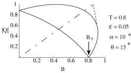
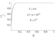
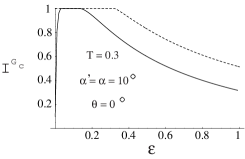
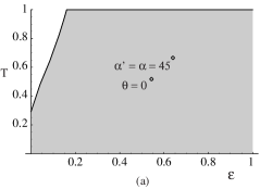
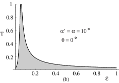
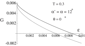
Now, since we have listed up all candidates for Eve’s optimum operation, we can obtain Eve’s maximum information gain by picking up the optimum one numerically. We show some examples of Eve’s information gain as a function of $\alpha^{\prime}$, $\alpha$, $T$, $\theta$, and $\epsilon$ in Fig. 6 and Fig. 7. In these figures, we plot Eve’s maximum information gain as a function of $\epsilon$. Since the parameter $\epsilon$ corresponds to the noise or the error rate, it might be expected that Eve’s information gain increases when $\epsilon$ gets larger. In Fig. 7, however, Eve’s information gain starts to decrease from the unity when the noise parameter $\epsilon$ exceeds a value around $0.13$. In Fig. 8, the shaded region represents the region where Eve’s information gain is unity when (a) $\alpha^{\prime}=\alpha=10^{\circ}$, and $\theta=0^{\circ}$, and (b) $\alpha^{\prime}=\alpha=45^{\circ}$ and $\theta=0^{\circ}$. We can see again in Fig. 8 (b) the counter-intuitive behavior that the Eve’s information gain is lower in the region with larger $\epsilon$.

Figure 6: Eve’s maximum information gain ${\rm I}^{\rm{Gc}}$ vs $\epsilon$ when $\alpha^{\prime}=\alpha=40^{\circ}$, $\theta=0^{\circ}$, and $T=0.8$.

Figure 7: Eve’s maximum information gain ${\rm I}^{\rm{Gc}}$ vs $\epsilon$ when $\alpha^{\prime}=\alpha=10^{\circ}$, $\theta=0^{\circ}$, and $T=0.3$. The dashed line is the information bound based on Eq. (61).

Figure 8: Eve’s information gain is unity in the gray region when (a) $\alpha^{\prime}=\alpha=40^{\circ}$, and $\theta=0$, and (b) $\alpha^{\prime}=\alpha=10^{\circ}$ and $\theta=0$.

In order to explain the counter-intuitive behavior in Fig. 7, let us consider the mutual information among the classical variables in Alice, Bob and Eve’s sites. Let $A$, $B$, and $E$ be the random variables describing Alice’s bit value (0 or 1), Bob’s measurement result ($\bar{0}$, $\bar{1}$, or inconclusive), and Eve’s classical data obtained from her attack, respectively. Let us consider the conditional mutual information ${\rm{I(E;A,B|{\rm{c}})}}\equiv H(A,B|{\rm{c}})-H(A,B|E,{\rm{c}})$, which is the mutual information between Eve and the joint system of Alice and Bob for conclusive bits. Here $c$ represents the condition that $B=\bar{0}$ or $\bar{1}$, meaning that Bob’s measurement result is conclusive. The function $H(A,B|{\rm{c}})$ represents the entropy of the joint system on condition that Bob obtains a conclusive result, and $H(A,B|E,{\rm{c}})$ stands for the conditional entropy of the joint system averaged over Eve’s variable $E$, namely, $H(A,B|E,{\rm{c}})\equiv\sum_{y}{\rm Prob}(E=y)H(A,B|E=y,{\rm{c}})$. Using the basic properties of the entropy function, we can easily see that the following relation holds:

$${\rm{I(E;A,B|{\rm{c}})}}+{\rm{I(A;B|{\rm{c}})}}={\rm{I(A;B,E|{\rm{c}})}}+{\rm{I(B;E|{\rm{c}})}}.$$ (53)

The information ${\rm{I(E;A,B|{\rm{c}})}}$ is, hence, bounded as follows:

$${\rm{I(E;A,B|{\rm{c}})}}\leq{\rm{I(A;B,E|{\rm{c}})}}+{\rm{I(B;E|{\rm{c}})}}.$$ (54)

The term ${\rm{I(A;B,E|{\rm{c}})}}$ in the right-hand side means how well the joint system of Bob and Eve can distinguish Alice’s states on condition that Bob obtains a conclusive result, and this term can be bounded from the fact that Alice’s states are nonorthogonal, as follows. With the help of the inequality

$${\rm{I(A;B,E)}}\geq P_{\rm{conc}}{\rm{I(A;B,E|{\rm{c}})}}+(1-P_{\rm{conc}}){\rm{I(A;B,E|{\rm{inc}})}}\,,$$ (55)

where “${\rm inc}$” means $B={\rm inconclusive}$ and $P_{\rm{conc}}$ is the probability that Bob obtains the conclusive results. For $\theta=0$ and $\alpha^{\prime}=\alpha$, $P_{\rm{conc}}$ is given by

$$P_{\rm{conc}}=\frac{T}{4}\left[2-(1-\epsilon)(\cos 2\alpha+1)\right]\,,$$ (56)

we can bound ${\rm{I(A;B,E|{\rm{c}})}}$ as

$${\rm{I(A;B,E|{\rm{c}})}}\leq\frac{{\rm{I(A;B,E)}}}{P_{\rm{conc}}}\leq\frac{1-h\left(\frac{1-\sqrt{1-\cos^{2}\alpha}}{2}\right)}{P_{\rm{conc}}}\,.$$ (57)

The second inequality in Eq. (57) comes from the optimum measurement on two nonorthognal pure states, which was mentioned in Sec. III.

The second term ${\rm{I(B;E|{\rm{c}})}}$ in the right-hand side of Eq.(54) means how well Eve can control Bob’s measurement outcomes, $B=\bar{0}$ and $B=\bar{1}$. Since Bob’s POVM elements $F_{\overline{0}}$ and $F_{\overline{1}}$ are nonorthogonal, Eve cannot control Bob’s outcome as she please, and ${\rm{I(B;E|{\rm{c}})}}$ generally decreases as $\alpha$ decreases. As we discuss the detail in Appendix C, ${\rm{I(B;E|{\rm{c}})}}$ is bounded by

$${\rm{I(B;E|{\rm{c}})}}\leq 1$$ (58)

$$- h\left(\frac{1}{2}-\frac{\sin\alpha}{4(P_{\rm{conc}}/T)}\sqrt{1-\left(\frac{2(P_{\rm{conc}}/T)-1}{\cos\alpha}\right)^{2}}\right)\,.$$

Combining Eqs. (54), (57), and (58), the mutual information ${\rm{I(E;A,B|{\rm{c}})}}$ is bounded by

$${\rm{I(E;A,B|{\rm{c}})}}\leq\frac{1-h\left(\frac{1-\sqrt{1-\cos^{2}\alpha}}{2}\right)}{P_{\rm{conc}}}$$ (59)

$$+ 1-h\left(\frac{1}{2}-\frac{\sin\alpha}{4(P_{\rm{conc}}/T)}\sqrt{1-\left(\frac{2(P_{\rm{conc}}/T)-1}{\cos\alpha}\right)^{2}}\right)$$

$$\equiv \nu$$

After the transmission of $n$ pulses from Alice to Bob, we expect $n_{\rm conc}\equiv nP_{\rm conc}$ conclusive events on average, and Eve’s information about Alice and Bob’s bits for these events is bounded by $nP_{\rm conc}\nu$. This quantity approaches zero when $\alpha$ goes to zero. On the other hand, Alice and Bob obtain $n_{\rm cor}\equiv nP_{\rm{conc}}(1-e)$ correct bits, where $e$ is the bit error rate given by

$$e=\frac{\epsilon}{2-(1-\epsilon)\,\left(\cos 2\alpha+1\right)}\,,$$ (60)

for $\theta=0$ and $\alpha^{\prime}=\alpha$. The number of correct bits $n_{\rm cor}$ does not necessarily approach zero when $\alpha$ goes to zero. The information gain per one correct bit, $\rm{I}^{Gc}_{S}$, cannot exceed $n_{\rm conc}\nu/n_{\rm cor}$, namely,

$${\rm{I}^{Gc}_{S}}\leq\frac{\nu}{1-e}\equiv\rm{I}^{upper}_{S}\,.$$ (61)

Since Shannon information gain ${\rm I}^{{\rm Gc}}_{{\rm S}}$ [Eq. (9)] and the information gain ${\rm{I}^{Gc}}$ [Eq. (7)] are connected by only one parameter $Q$, we can bound ${\rm{I}^{Gc}}$ through $\rm{I}^{upper}_{S}$. In Fig. 7, we plot this information bound by the dashed line. The dashed line decreases as $\epsilon$ gets larger.

To summarize, the counter-intuitive behavior can be explained as follows. When $\alpha$ is small, Alice’s bit value cannot be guessed well from the outside since she encodes it into nonorthogonal states. Bob’s measurement results are also hard to guess since they come from nonorthogonal measurements. As a result, the mutual information between Alice and Bob, $\rm{I(A;B|c)}$, and Eve’s information $\rm{I(E;A,B|c)}$, are both upper-bounded by the quantity $\nu$, which approaches zero when $\alpha$ goes to zero. On the other hand, when $\epsilon$ is large, the number of the conclusive bits is not small even when $\alpha$ is close to zero. This means that Alice’s bits and Bob’s bits for the conclusive bits are almost uncorrelated when $\alpha$ is close to zero. Then, Alice and Bob construct the correct bits by picking up the bits whose values accidentally coincide, through the encrypted communication over the classical channel. In this case, the correct bits are essentially generated in this encrypted transmission, and Eve’s information gain about them is very low. It is, however, not practical to perform quantum key distribution in this region, since Alice and Bob must use many bits of the initially shared secret key to determine the correct bits.

Figure 9: Eve’s information gain is unity in the gray region $\{\alpha,\epsilon\}$ for $T=1$ and $\theta=0$.

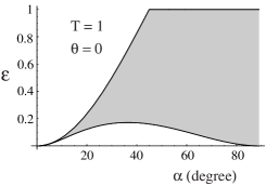
Figure 9 shows in gray the region where Eve’s information gain is unity in the parameter region $\{\alpha,\epsilon\}$ for $T=1,\theta=0,\alpha^{\prime}=\alpha$. The upper-left white region (small $\alpha$ and large $\epsilon$) corresponds to the counter-intuitive behavior we have just discussed. The figure shows another interesting behavior for small $\epsilon$; Eve’s information gain is unity only when $\alpha$ is small or large, and is not unity for intermediate values of $\alpha$. For $T<1$, the region for the full information gain for Eve has a similar shape to Fig. 9, but is wider because the transmission loss gives advantage to Eve. In order to understand this behavior at $T=1$, we consider the following specific individual attack that gives Eve the perfect information about the correct bits.

If Eve is sure that the state $|1\rangle(=|\sigma_{\alpha}\rangle)$ released by Alice always evolves to $|0\rangle(=|\sigma_{-\alpha}\rangle)$ and then reaches Bob, Eve can be sure that the value of the conclusive bit surviving the error discarding procedure is 0. The simplest way to perform this attack is to rotate the system counter-clockwise by angle $2\alpha$ in the Bloch sphere (see Fig. 1). To keep the symmetry, for half of the cases Eve rotates the system by angle $-2\alpha$. For the latter cases she can be sure that the value of the correct bit is $1$. In this attack, the averaged state $\rho^{\rm s}_{1}$ received by Bob when Alice has emitted $|1\rangle$ is given by $\rho^{\rm s}_{1}=(|\sigma_{-\alpha}\rangle\langle\sigma_{-\alpha}|+|\sigma_{2\alpha}\rangle\langle\sigma_{2\alpha}|)/2=\cos^{2}\alpha|\sigma_{\alpha}\rangle\langle\sigma_{\alpha}|+\sin^{2}\alpha|\overline{\sigma_{\alpha}}\rangle\langle\overline{\sigma_{\alpha}}|$. This attack is thus successful when $\epsilon=2\sin^{2}\alpha$, which coincides with the upper boundary in Fig. 9.

The above “rotating” strategy can be improved by performing a weak measurement before the rotation, so that it can be used for smaller values of $\epsilon$. The weak measurement with outcomes $\{+,-\}$ is described by the POVM $\{\hat{A}_{+},\hat{A}_{-}\}$, where

$$\hat{A}_{+}=(1-q)|x+\rangle\langle x+|+q|x-\rangle\langle x-|$$ (62)

and

$$\hat{A}_{-}=q|x+\rangle\langle x+|+(1-q)|x-\rangle\langle x-|\,.$$ (63)

The parameter $q$ $(0\leq q\leq 1/2)$ represents the weakness of the measurement. If Alice has emitted $|j\rangle$ $(j=0,1)$, the outcome “$+$” and “$-$” occur with probability $p_{j+}\equiv\langle j|\,\hat{A}_{+}|j\rangle$ and $P_{j-}\equiv\langle j|\,\hat{A}_{-}|j\rangle$, respectively. When this weak (projection) measurement produced outcome “$+$”, the angle $\beta$ (in the Bloch sphere) between the postmeasurement states $\sqrt{\hat{A}_{+}}|0\rangle$ and $\sqrt{\hat{A}_{+}}|1\rangle$ is given by

$$\cos^{2}(\beta/2)=|\langle 0|\hat{A}_{+}|1\rangle|^{2}/(p_{0+}p_{1+}).$$ (64)

The outcome “$-$” gives the same angle by the symmetry. The angle $\beta$ is monotone increasing from $0$ to $2\alpha$ as a function of $q\in[0,1/2]$.

After this measurement, Eve rotates the system depending on the outcome. For “$+$”, she rotates it so that $\sqrt{\hat{A}_{+}}|0\rangle$ becomes $|1\rangle$. The state $\sqrt{\hat{A}_{+}}|1\rangle$ moves to $|\sigma_{\alpha+\beta}\rangle$ in this rotation. When the outcome is “$-$”, she rotates it so that $\sqrt{\hat{A}_{+}}|1\rangle$ becomes $|0\rangle$. In this attack, the averaged state $\rho^{\rm s}_{1}$ received by Bob when Alice has emitted $|1\rangle$ is given by $\rho^{\rm s}_{1}=p_{1-}|\sigma_{-\alpha}\rangle\langle\sigma_{-\alpha}|+p_{1+}|\sigma_{\alpha+\beta}\rangle\langle\sigma_{\alpha+\beta}|$. This state can be written in the form $(1-\epsilon/2)|\sigma_{\alpha}\rangle\langle\sigma_{\alpha}|+(\epsilon/2)|\overline{\sigma_{\alpha}}\rangle\langle\overline{\sigma_{\alpha}}|$ when

$$\sin{\beta}/\sin{2\alpha}=p_{1-}/p_{1+}$$ (65)

holds. In such a case, the value of $\epsilon$ is given by

$$\epsilon=1-\frac{\sin(2\alpha+\beta)}{\sin 2\alpha+\sin\beta}.$$ (66)

The equation (65) has two solutions in $q\in[0,1/2]$, $q=q_{0}(\alpha)$ and $q=1/2$. The case of $q=1/2$ corresponds to the simple rotating strategy described before. The strategy corresponding to the other solution $q=q_{0}(\alpha)$ turns out to give the lower boundary in Fig. 9. The entire gray region in Fig. 9 is then covered by simply mixing the two strategies corresponding to $q=q_{0}(\alpha)$ and $q=1/2$.

The behavior for small $\epsilon$ shown in Fig. 9 will now be understood as follows. When $\alpha$ is small, the simple rotating strategy with the small rotation angle $2\alpha$ causes only a small disturbance, and it can be used to obtain small $\epsilon$. When $\alpha$ is large and the two states can be well distinguished, the improvement of the strategy by the measurement is quite effective to reduce $\epsilon$. For intermediate values of $\alpha$, $p_{0+}/p_{1+}$ cannot be close to zero. Since $p_{0+}=p_{1-}$, the angle $\beta$ cannot be close to zero either, due to the constraint (65). Consequently, as is implied by Eq. (66), even the improved strategy cannot reduce $\epsilon$ close to zero.

VI Secret Key Gain

In this section, we show the calculation of secret key gain and the optimum angle of Alice’s states to obtain optimum secret key gain. For simplicity, we assume that $\alpha=\alpha^{\prime}$ and $\theta=0$. The calculation for more general cases is straghtforward.

We define the secret key gain $G$ as the net growth of the secret key per one pulse. Alice and Bob can increase the length of the secure secret key in the region where $G$ is positive.

In the calculation of key gain, we assume the error correction protocol whose number of redundancy bits used to detect the errors of the raw key are equal to the Shannon limit, i.e., $nh(e)$, where $n$ is the length of the raw key, $e$ is the bit error rate of the raw key given by Eq. (60), and $h(e)$ is entropy function. We further assume that the privacy amplification privacy amp is applied to the correct bits and to the flipped bits independently. Since Eve may not be allowed to adopt the strategy that is simultaneously optimum both for correct bits and flipped bits, this protocol may be overkill but never underestimates Eve’s ability.

For the privacy amplification of the correct bits, we use Eve’s information estimated via the method described in the previous sections. From these bits Alice and Bob obtain $G^{\rm new}_{c}$ bits per pulse of new secret key, which is written as

$$G^{\rm new}_{c}\equiv P_{{\rm conc}}(1-e)(1-{\rm I}^{{\rm Gc}})-(s_{c}/n_{{\rm total}})\,$$ (67)

where $P_{{\rm conc}}$ is given by Eq. (56), $n_{{\rm total}}$ is the number of pulses emitted by Alice, and $s_{c}$ is the security parameter for correct bits. Eve’s information about the secret key obtained from the correct bits is less than $2^{-s_{c}}/\ln 2$ (bits).

For flipped bits, Alice and Bob obtain $G^{\rm new}_{f}$ bits per pulse of new secret key, which is written as

$$G^{\rm new}_{f}\equiv P_{{\rm conc}}e(1-{\rm I}^{{\rm Gf}})-(s_{f}/n_{{\rm total}})\,.$$ (68)

Eve has information less than $2^{-s_{f}}/\ln 2$ (bits) about the secret key from the flipped bits. The information gain for flipped bits $\rm{I}^{{\rm Gf}}$ can directly be obtained by replacing $\theta$ with $-2\alpha-\theta$ in the formula in Sec. IV.

Noting that the redundancy bits used in the error correction protocol are encrypted by consuming $P_{{\rm conc}}h(e)$ bits per pulse of the initially shared secret key, we obtain the expression of the secret key gain $G$ as follows,

$$G \equiv G^{\rm new}_{c}+G^{\rm new}_{f}-P_{{\rm conc}}h(e)$$ (69)

$$= P_{{\rm conc}}\left[(1-e)(1-{\rm I}^{{\rm Gc}})+e(1-{\rm I}^{{\rm Gf}})-h(e)\right]$$

$$- (s_{c}+s_{f})/n_{{\rm total}}\,.$$

In the limit of long key, i.e., $n_{{\rm total}}\to\infty$, $G$ is reduced to

$$G=P_{{\rm conc}}\left[(1-e)\,(1-{\rm I}^{{\rm Gc}})+e(1-{\rm I}^{{\rm Gf}})-h(e)\right]\,.$$ (70)

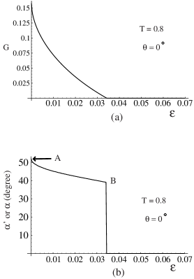
In B92 protocol, if $\alpha^{\prime}(=\alpha)$ is changed, the secret key gain will be changed. So, Alice and Bob should optimize this angle to obtain higher secret key gain. In Fig. 10, we optimize $\alpha^{\prime}\,(=\alpha)$ for fixed values of $T$ and $\epsilon$ gene to obtain high secret key gain, and plot the key gain and the optimized angle as a function of $\epsilon$. The points “A” and “B” represent the cases when $\epsilon=0$ and when the key gain vanishes, respectively. In the figure, as $\epsilon$ increases, the optimum angle tends to be smaller, and the region where optimum angle $\alpha^{\prime}=0$ implies that our protocol does not work. In the figure, there is only a negligible contribution of flipped bits to the key gain.

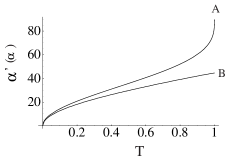
To investigate the $T$ dependence on the optimum angle which are represented as “A” and “B”, we plot these angles as a function of $T$ in Fig. 11. For “A”, the key gain has a simple expression

$$G=\frac{T}{4}(1-\cos 2\alpha^{\prime})\left[1-\log_{2}\left(2-\left(\frac{\cos\alpha^{\prime}-1+T}{T\cos\alpha^{\prime}}\right)^{2}\right)\right]\,.$$ (71)

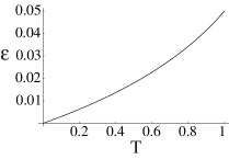
In Fig. 11, it is seen that as $T$ gets larger, the optimum angle tends to get larger. In Fig. 12, we plot $\epsilon$ of “B” as a function of $T$. The region below the curve means the parameter region of $\{T,\epsilon\}$ where a secure key can be produced in our protocol.

Figure 10: (a) The optimized secret key gain per pulse and (b) optimal angle $\alpha^{\circ}$ as a function of $\epsilon$. $T=0.8$, $\alpha^{\prime}=\alpha$ and $\theta=0^{\circ}$. “A” represents the angle when $\epsilon=0$ and “B” represents the angle when the key gain vanishes.

Figure 11: The $T$ dependence of“A” and “B”.

Figure 12: The maximum value of $\epsilon$ up to which the secret key gain is positive as a function of $T$.

Finally, to compare the security of B92 with that of BB84 assuming an ideal single-photon source, we consider the dependence of $G$ as a function of distance between Alice and Bob, while imperfection factors such as dark counting of detectors and losses of optical fibers are fixed. For the purpose of this comparison, we consider the case where Bob uses photon counters which can discriminate no photon, single-photon, and higher number of photons. Let $l$, $L_{c}$, $L_{r}$, $\nu$, and $\eta$ be the length of transmission line (km), the channel loss (dB/km), the receiver loss (dB), the mean dark count per pulse (which is given by $\nu=\tau_{{\rm res}}R_{{\rm dark}}$ where $R_{{\rm dark}}$ is the dark counting rate and $\tau_{{\rm res}}$ is the resolution time of the detector and electronic circuitry), and the detection efficiency, respectively. In this case, $T$ is given by barnett

$$T={\rm e}^{-\nu}\,\eta\,10^{-(lL_{c}+L_{r})/10}+{\rm e}^{-\nu}\,\nu(1-10^{-(lL_{c}+L_{r})/10})\,,$$ (72)

where we assume that the dark counts are Poissonian events. From this equation and

$$\tilde{\rho}_{i}^{{\rm s}} = \frac{{\rm e}^{-\nu}\,\eta\,10^{-(lL_{c}+L_{r})/10}}{T}|i\rangle\langle i|$$ (73)

$$+ \frac{{\rm e}^{-\nu}\,\nu(1-10^{-(lL_{c}+L_{r})/10})}{T}\frac{\textbf{1}}{2}$$

$$= (1-\epsilon)|i\rangle\langle i|+\frac{\epsilon}{2}\,{\textbf{1}}\,,$$

$\epsilon$ can be written as

$$\epsilon=\frac{\,{\rm e}^{-\nu}\,\nu(1-10^{-(lL_{c}+L_{r})/10})}{T}\,.$$ (74)

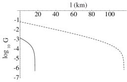
In Fig. 13, we plot $\log_{10}G$ as a function of distance $l$(km). In the figure, we put $\alpha(\alpha^{\prime})=11$(degree) which is almost optimum, and experimental data is taken from KTH KTH . For the secret key gain of BB84 protocol in the figures, we used the formula for the single-photon case in norbert2 ,

$$G = \frac{T}{2}[1-\log_{2}(1+4e-4e^{2})+e\log_{2}e$$ (75)

$$+ (1-e)\log_{2}(1-e)]\,,$$

where $e=\nu/(2T)$, assuming that the errors stem from the dark counting. In Fig. 13, it is seen that B92 protocol is far less efficient, which is mainly because a low transmission rate $T$ directly gives an advantage to Eve in the B92 scheme using photon polarization.

Figure 13: Comparison of B92 (solid line) with BB84 (dotted line) in the case where $L_{c}=0.2$(dB), $L_{r}=1$(dB), $\nu=2\times 10^{-4}$(per pulse), and $\eta=18$ (%). The dotted line represents BB84 and solid line represents B92 protocol.

VII Summary and Discussion

Throughout this paper, we have estimated Eve’s information gain ${\rm I}^{{\rm Gc}}$. But as Bennett et al. pointed out in Sec. VI of privacy amp , if eavesdropping is independently done for each pulse, privacy amplification using information gain based on the expected collision probability is overkill. In such case, it follows that it may be sufficient to estimate Eve’s information gain by Shannon entropy. In the case where Eve employs the symmetric von Neumann measurement, the proof in privacy amp assures that Shannon entropy is enough for the estimation. Maximizing Eve’s information gain with respect to Shannon entropy is equivalent to the problem of minimizing $|Q|^{2}$, which is the same problem as the maximization of Eve’s information gain ${\rm I}^{{\rm Gc}}$. So, our method described in the previous sections can be directly applied to this problem. We plot an example of the secret key gain for some cases when we estimate Eve’s maximum information gain by Shannon entropy in Fig. 14. We see that the key gain is higher than the case where Eve’s information is estimated by ${\rm I}^{{\rm Gc}}$.

Another candidate which may make the key gain higher is error reconciliation protocols. There may be the case where error discarding protocols error discarding are more efficient than the error correction protocol, because the redundancy bits consumed in a discarding protocol may be less, for Alice and Bob do not need to keep the discarded bits secret in the error discarding protocol. In the calculation of all figures in Sec. VI, we have checked that there is no contribution of the flipped bits to the secret key, which implies that the use of an error discarding protocol may be more efficient than that of an error correction protocol.

Figure 14: The secret key gain vs $\epsilon$ in the case of $T=0.3$, $\alpha^{\prime}=\alpha=12^{\circ}$ and $\theta=0^{\circ}$. Eve’s information is estimated by Shannon entropy (solid line) and ${\rm I}^{{\rm Gc}}$ (dotted line). The estimation by Shannon entropy is more efficient.

Since the density matrices which Alice emits are fixed as well as those which are received by Bob, the problem of our estimation of quantum key distribution over a realistic channel is reduced to the problem that how much information Eve can extract on the condition that both initial density matrices $\rho_{i}$ ($i=0,1$) and final density matrices $\rho_{i}^{\prime}$ are fixed. In the realistic situation, however, since the number of pulses $n_{\rm total}$ which are emitted by Alice is finite, we cannot uniquely identify the final density matrices. In such a situation, by considering the standard deviation of Bob’s data, we can pick up the candidates of the final density matrices, and we can estimate Eve’s maximum information gain by comparing information gain for each candidates.

To summarize this paper, we derived a formula that estimates Eve’s maximum information when Alice and Bob perform B92 protocol using two nonorthogonal single-photon polarization states. We have assumed that Alice can emit a single photon and Eve employs individual attack. The problem is equivalent to ask how much information can be extracted while simulating a noisy channel through which Alice communicates with Bob by sending the two nonorthogonal states. The dependence of the maximum information on the noise parameter shows nontrivial behavior. It decreases as the noise increases in some parameter regions. For a small noise rate, Eve can extract perfect information in the case where the angle of Alice’s two states is very small or very large, while she cannot extract perfect information for intermediate angles. Using the formula, we plot the secret key gain as a function of various parameters reflecting intervention by Eve. We also investigated the optimum angle between the two states to obtain large secret key gain, and showed the region of the parameters where this key gain is positive. A comparison of our protocol with BB84 protocol shows that B92 protocol with single photon polarization is less efficient than BB84 protocol, which is mainly because a low transmission rate $T$ directly gives an advantage to Eve in the B92 scheme using photon polarization. This drawback may be compensated in the original B92 protocol using two nonorthogonal coherent light, or in the 4+2 protocol imoto that uses the switching of the basis as in BB84 while retaining the nonorthgonality as a freely adjustable parameter. We leave the security problems of such protocols to future studies.

We have assumed throughout this paper that eavesdropping is independent for each pulse. Even within the independent quantum operation, Eve can obtain a correlation among her eavesdropping outcomes by choosing her strategy depending on the outcomes which have been already obtained. The estimation against such attack is important for the realistic purpose, but we also leave this problem for future studies, along with the security against collective attack or coherent attack.

Appendix A Symmetrization of Eve’s strategy

In this appendix, we construct a symmetrized strategy $U^{\rm s}$, which possesses higher symmetry and the same power as the actual strategy $U$, namely, $|Q(U^{\rm s})|=|Q(U)|$. The problem of minimizing $|Q|$ over possible $U$ is then simplified to the minimization over possible $U^{\rm s}$. Similar discussion is seen in Appendix A of slu . In addition to the symmetry, this reduction makes the analysis simpler because the states delivered to Bob by the strategy $U^{\rm s}$ are completely specified by the observed quantities.

First, consider a strategy $U^{\prime}$ in which Eve conducts an additional (nondestructive) measurement of the photon number just after the original strategy of $U$ satisfying Eqs. (5) and (10). After this measurement, if the outcome of this measurement is one photon, she sends the projected state to Bob, but if the outcome is no photon or more than one photon, she always sends the vacuum state $|\,{\rm vac}\,\rangle$. The states $\rho_{j}^{\prime}(j=0,1)$ delivered to Bob in this strategy are given by

$$\rho_{j}^{\prime}=P_{1}\rho_{j}P_{1}+(1-T_{j})\,|\,{\rm vac}\,\rangle\langle{\rm vac}\,|,$$ (76)

where $P_{1}$ is the projection onto the subspace $H_{1}$ of one photon and

$$T_{j}\equiv 1-{\rm Tr}[F_{\rm V}\rho_{j}]\,,$$ (77)

which is the probability that Bob detects a single-photon. Since ${\rm Tr}(F_{\mu}\rho_{j}^{\prime})={\rm Tr}(F_{\mu}\rho_{j})$ $(\mu=0,1,\bar{0},\bar{1};j=0,1)$, the strategy $U^{\prime}$ satisfies the condition Eq. (5), and the additional measurement only gives Eve extra information, $|Q(U^{\prime})|\leq|Q(U)|$ holds. Hence, in finding the minimum of $|Q(U)|$ under the condition Eq. (5), we are allowed to assume the additional assumption that $\rho_{j}$ is equal to $\rho_{j}^{\prime}$ and is written as

$$\rho_{j}=T_{j}\tilde{\rho}_{j}+(1-T_{j})\,|\,{\rm vac}\,\rangle\langle{\rm vac}\,|,$$ (78)

where $\tilde{\rho}_{j}\equiv P_{1}\rho_{j}P_{1}/T_{j}$ is a normalized density operator in $H_{1}$.

Next, take a basis of the signal space $H$ that includes $|\,z+\rangle$, $|\,z-\rangle$, and $|\,{\rm vac}\,\rangle$ as elements, and take a basis of Eve’s probe space that includes $|\,w\,\rangle$. The product states of the two bases form a basis of the combined system, and let us denote it as ${\rm W}$. Let $Z_{{\rm W}}$ be the transformation which replaces all the vector components and the elements of matrices in the basis ${\rm W}$ with their complex conjugates. Since the initial states $|\,j\,\rangle\,|\,w\rangle_{\rm E}(j=0,1)$ and Bob’s measurement $\{F_{\mu}\}$ are invariant under the transformation $Z_{{\rm W}}$, and the probabilities of events in quantum mechanics are given by moduli squared of vector inner products, the strategy given by the unitary operator $Z_{{\rm W}}UZ_{{\rm W}}^{-1}$ gives the same amount of the information gain to Eve as the strategy $U$.

Similarly, let $\sigma_{z}\equiv|z+\rangle\langle z+|-|z-\rangle\langle z-|$ be the $\pi$ rotation around the $z$ axis in the Bloch sphere, and $R$ be the extension of $\sigma_{z}$ to the entire space ($R\equiv(\sigma_{z}\oplus F_{{\rm V}})\otimes 1_{\rm E}$, where subscript E means Eve’s probe space). Since the changes in the initial states $|\,j\,\rangle\,|\,w\,\rangle_{\rm E}(j=0,1)$ and Bob’s measurement $\{F_{\mu}\}$ under the transformation $R$ is just the interchange of the bit values $0$ and $1$, the strategy given by the unitary operator $RUR^{-1}$ gives the same amount of the information gain to Eve as the strategy $U$.

Since the four strategies $U$, $Z_{{\rm W}}UZ_{{\rm W}}^{-1}$, $RUR^{-1}$, and $RZ_{{\rm W}}UZ_{{\rm W}}^{-1}R^{-1}$ give the same amount of information gain, the strategy in which Eve randomly chooses one of the four unitary operations also gives the same amount of information gain. In other words, if we write the unitary operator corresponding to this randomized strategy as $U^{\rm s}$, then $|Q(U^{\rm s})|=|Q(U)|$ holds. The states $\rho_{0}^{\rm s}$ and $\rho_{1}^{\rm s}$ delivered to Bob in this strategy are given by

$$\rho_{0}^{\rm s} = \frac{1}{4}({\rho}_{0}+Z_{{\rm W}}\rho_{0}Z_{{\rm W}}^{-1}+R\rho_{1}R^{-1}$$ (79)

$$+ Z_{{\rm W}}R\rho_{1}R^{-1}Z_{{\rm W}}^{-1})$$

$$= T\tilde{\rho}_{0}^{\rm s}+(1-T)|{\rm vac}\rangle\langle{\rm vac}|$$

and

$$\rho_{1}^{\rm s} = \frac{1}{4}({\rho}_{1}+Z_{{\rm W}}\rho_{1}Z_{{\rm W}}^{-1}+R\rho_{0}R^{-1}$$ (80)

$$+ Z_{{\rm W}}R\rho_{0}R^{-1}Z_{{\rm W}}^{-1})$$

$$= T\tilde{\rho}_{1}^{\rm s}+(1-T)|{\rm vac}\rangle\langle{\rm vac}|,$$

where

$$\tilde{\rho}_{0}^{\rm s} = \frac{1}{4T}[T_{0}(\tilde{\rho}_{0}+Z_{{\rm W}}\tilde{\rho}_{0}Z_{{\rm W}}^{-1})+T_{1}(R\tilde{\rho}_{1}R^{-1}$$ (81)

$$+ Z_{{\rm W}}R\tilde{\rho}_{1}R^{-1}Z_{{\rm W}}^{-1})],$$

$$\tilde{\rho}_{1}^{\rm s}=\sigma_{z}\tilde{\rho}_{0}^{\rm s}\sigma_{z}\,,$$ (82)

and

$$T\equiv\frac{T_{0}+T_{1}}{2}=1-{\rm Tr}[F_{\rm V}(\rho_{0}+\rho_{1})/2]\,.$$ (83)

From these expressions, we have

$${\rm Tr}[\sigma_{y}\tilde{\rho_{j}}^{\rm s}]=0,$$ (84)

where $\sigma_{y}\equiv i|z-\rangle\langle z+|-i|z+\rangle\langle z-|$. Eqs.(79) and (84) implies that $\tilde{\rho}_{j}^{\rm s}$ are written in the Bloch sphere as in Fig. 4. Taking the parameters $\theta$ and $\epsilon$ as in Fig. 4 (the sign of $\theta$ is positive in the clockwise), $\rho_{j}^{\rm s}$ can be written in a diagonalized form as in Eqs. (LABEL:den1) and (13).

Appendix B Optimization of Eve’s apparatus

In this appendix, we derive Eq. (39). In order to determine the function $Q_{\rm min}(B)$, we use Lagrange’s method of undetermined multipliers. $B_{0}$ is the maximum of $B(\hat{\xi})$ under the condition that $Q(\hat{\xi})=0$. Hence, if $B(\hat{\xi})=B_{0}$ and $Q(\hat{\xi})=0$, such $\hat{\xi}$ satisfies

$$\delta(B(\hat{\xi})-\nu Q(\hat{\xi}))=0$$ (85)

for any variation of $\hat{\xi}$. $Q_{\rm min}(B)$ for $B_{0}<B\leq B_{\rm max}$ is determined by minimizing $Q^{2}(\hat{\xi})$ under the condition that $B(\hat{\xi})=B$. Suppose that $Q^{2}(\hat{\xi})$ takes its minimum at $\hat{\xi}$ under the condition that $B(\hat{\xi})$ is fixed. Then, at least one of the following conditions holds, namely,

$$\delta B(\hat{\xi})=0$$ (86)

for any variation of $\hat{\xi}$, or, there exists real $\lambda^{\prime}$ such that

$$\delta(Q^{2}(\hat{\xi})-\lambda^{\prime}B(\hat{\xi}))=0$$ (87)

for any variation of $\hat{\xi}$. Since $Q(\hat{\xi})\neq 0$ in the considered region, the condition (87) is equivalent to

$$\delta(Q(\hat{\xi})-\lambda B(\hat{\xi}))=0\,,$$ (88)

where $\lambda\equiv\lambda^{\prime}/2Q$. The three conditions (85), (86), and (88) can be cast into a common form, namely, there exist real $\nu$ and $\lambda$ [$(\nu,\lambda)\neq(0,0)$] such that

$$\delta(\nu Q(\hat{\xi})-\lambda B(\hat{\xi}))=0$$ (89)

for any variation of $\hat{\xi}$. In determining $B_{0}$ and $Q_{\rm min}(B)$, it is sufficient to consider only the operator $\hat{\xi}$ satisfying the above condition.

Since $\hat{\xi}$ is a real orthogonal matrix in the basis ${\rm W}$, any variation of $\hat{\xi}$ can be written as $\hat{\xi}\rightarrow\hat{\xi}\,(1+\hat{N}\delta)$, where $\hat{N}$ is an arbitrary real antisymmetric matrix in ${\rm W}$ and $\delta$ is an infinitesimal real number. Then, the condition (89) means

$${\rm Tr}\left[(\nu\hat{A}-\lambda\hat{B})\,\hat{\xi}\,\hat{N}\right]=0$$ (90)

for any $\hat{N}$ whose matrix form in ${\rm W}$ is real and antisymmetric. This condition is satisfied if and only if $(\nu\hat{A}-\lambda\hat{B})\,\hat{\xi}$ is a real symmetric matrix in ${\rm W}$. Since $(\nu\hat{A}-\lambda\hat{B})$ is a real symmetric matrix and $\hat{\xi}$ is a real orthogonal matrix in ${\rm W}$, we have

$$(\nu\hat{A}-\lambda\hat{B})\,\hat{\xi}=\hat{\xi}^{-1}(\nu\hat{A}-\lambda\hat{B})$$ (91)

and hence

$$[(\nu\hat{A}-\lambda\hat{B})^{2},\hat{\xi}]=0.$$ (92)

Appendix C The upper bound of ${\rm{I(B;E|{\rm{c}})}}$

In this appendix, we derive an upper bound of ${\rm{I(B;E|{\rm{c}})}}$ in Eq. (58), assuming that Eve freely prepares quantum states and sends them to Bob. We only require that Eve should not change the values $T$ and $P_{\rm conc}$. Hence, Eve’s strategy is generally described as she sends a single photon with its polarization in the state $\rho_{\gamma}$ with probability $P(\gamma)T$, and she sends the vacuum with probability $1-T$. The probability $P(\gamma)$ should satisfy

$$\sum_{\gamma}P(\gamma)=1\,,$$ (93)

and $\rho_{\gamma}$ and $P(\gamma)$ should satisfy

$$\sum_{\gamma}P(\gamma)P({\rm{c}}|\gamma)=P_{\rm{conc}}/T\,.$$ (94)

Here $P({\rm{c}}|\gamma)$ is the probability of obtaining conclusive results for the state $\rho_{\gamma}$, which is given by

$$P({\rm{c}}|\gamma) = {\rm{Tr}}\left[(F_{\overline{0}}+F_{\overline{1}})\rho_{\gamma}\right]$$ (95)

$$= {\rm{Tr}}\left[\left(\cos^{2}\frac{\alpha}{2}|z+\rangle\langle z+|+\sin^{2}\frac{\alpha}{2}|z-\rangle\langle z-|\right)\rho_{\gamma}\right]$$

$$= \frac{1}{2}\left[1-\cos\alpha{\rm{Tr}}(\sigma_{z}\rho_{\gamma})\right]\,.$$

The mutual information ${\rm{I(B;E|{\rm{c}})}}$ can be written as

$${\rm{I(B;E|{\rm{c}})}} = H(B|{\rm{c}})-H(B|E,{\rm{c}})$$ (96)

$$\leq 1-\left(\frac{T}{P_{{\rm conc}}}\sum_{\gamma}P(\gamma)P({\rm{c}}|\gamma)H(B|\gamma,{\rm{c}})\right)\,.$$

The entropy $H(B|\gamma,{\rm{c}})$ is given by

$$H(B|\gamma,{\rm{c}}) = h\left(\frac{1}{2}-\frac{\left|P(\overline{0}|\gamma,{\rm{c}})-P(\overline{1}|\gamma,{\rm{c}})\right|}{2}\right)$$ (97)

$$= h\left(\frac{1}{2}-\frac{\left|{\rm{Tr}}[(F_{\overline{0}}-F_{\overline{1}})\rho_{\gamma}]\right|}{2P({\rm{c}}|\gamma)}\right).$$

Using

$$F_{\overline{0}}-F_{\overline{1}}=\frac{\sin\alpha}{2}\sigma_{x}$$ (98)

and the relation ${\rm{Tr}}(\sigma_{z}\rho_{\gamma})^{2}+{\rm{Tr}}(\sigma_{x}\rho_{\gamma})^{2}\leq 1$, we obtain

$$H(B|\gamma,{\rm{c}}) \geq h\left(\frac{1}{2}-\frac{\sin\alpha}{4P({\rm{c}}|\gamma)}\sqrt{1-\left(\frac{1-2P({\rm{c}}|\gamma)}{\cos\alpha}\right)^{2}}\right)$$ (99)

$$\equiv g\left(P({\rm{c}}|\gamma)\right)\,,$$

Since the function $x\rightarrow xg(x)$ is convex (we have confirmed this numerically), ${\rm{I(B;E|{\rm{c}})}}$ in Eq. (96) is maximum when $P({\rm{c}}|\gamma)=P_{\rm{conc}}/T$ for all $\gamma$, and we obtain the result

$${\rm{I(B;E|{\rm{c}})}}\leq 1-g\left(P_{\rm{conc}}/T\right),$$ (100)

which is Eq. (58).

References

- (1) C. H. Bennett and G. Brassard, in Proceeding of the IEEE International Conference on Computers, Systems, and Signal Processing, Bangalore, India (IEEE, New York, 1984), pp.175-179 (1984).
- (2) A. K. Ekert, Phys. Rev. Lett, 67, 661 (1991).
- (3) C. H. Bennett, Phys. Rev. Lett, 68, 3121 (1992).
- (4) B. Huttner, N. Imoto, N. Gisin, and T. Mor, Phys. Rev. A51, 1863 (1995), L. Goldenberg and L. Vaidman, Phys. Rev. Lett, 75, 1239 (1995), M. Koashi and N. Imoto, Phys. Rev. Lett, 79, 2383 (1997).
- (5) H.-K. Lo and H. F. Chau, quant-ph/9803006.
- (6) D. Mayers, quant-ph/9802025.
- (7) E. Biham, M. Boyer, P. O. Boykin, T. Mor, and V. Roychowdhury, quant-ph/9912053.
- (8) P. W. Shor and J. Preskill, Phys. Rev. Lett, 85, 441 (2000).
- (9) H. Inamori, N. Ltkenhaus, and D. Mayers, quant-ph/0107017.
- (10) C. H. Bennett, D. P. DiVincenzo, J. A. Smolin, and W. K. Wootters, Phys. Rev. A 54, 3824 (1996).
- (11) A. R. Calderbank and P. W. Shor, Phys. Rev. A 54, 1098 (1996), A. M. Steane, Proc. R. Soc. London A 452, 2551 (1996),
- (12) H. -K. Lo, quant-ph/0102138,
- (13) N. Ltkenhaus, Phys. Rev. A 61, 052304 (2000).
- (14) E. Waks, A. Zeevi, and Y. Yamamoto, quant-ph/0012078.
- (15) C. A. Fuchs and A. Peres, Phys. Rev. A 53, 2038 (1996).
- (16) B. A. Slutsky, R. Rao, P.-C. Sun, and Y. Fainman, Phys. Rev. A, 57, 2383 (1998).
- (17) N. Ltkenhaus, Phys. Rev. A 59, 3301 (2000).
- (18) C. H. Bennett, G. Brassard, C. Crpeau, and U. M. Maurer, IEEE Trans. Inf. Theory 41, 1915 (1995).
- (19) L. B. Levitin, in Quantum Communication and Measurement, edited by V. P. Belavkin, O. Hirota, and R. Hudson (Plenum, New York, 1995), pp.439-448.
-
(20)
J. Preskill,
http://www.theory.caltech.edu/people/preskill/ph229/ . - (21) M. N. Wegman and J. L. Carter, J. Comp. Syst. Sci. 22, 265 (1981).
- (22) Although the Appendix B of slu claims that the expected Renyi entropy is maximized by the symmetric von Neumann measurement, they have also proved in their proof an inequality, which reads in our notation, showing that the expected collision probability is also maximized by the symmetric von Neumann measurement.
- (23) C. H. Bennett, F. Bessette, G. Brassard, L. Salvail and J. Smolin, J. Cryptology, 5, 3 (1992).
- (24) In general, there exist correlations among , , , and . But since we can calculate Eve’s information gain for any , , , , and , even if such a correlation exists, Alice and Bob can maximize the secret key gain by taking this correlation into consideration.
- (25) S. M. Barnett, L. S. Phillips, and D. T. Pegg, Opt. Comm. 158, 45 (1998).
- (26) M. Bourennane, F. Gibson, A. Karlsson, A. Hening, P. Jonsson, T. Tsegaye, D. Ljunggren, and E. Sundberg, Opt. Express 4, 383 (1999).