Three-dimensional Casimir force between absorbing multilayer dielectrics

Abstract

Recently the influence of dielectric and geometrical properties on the Casimir force between dispersing and absorbing multilayered plates in the zero-temperature limit has been studied within a 1D quantization scheme for the electromagnetic field in the presence of causal media [R. Esquivel-Sirvent, C. Villarreal, and G.H. Cocoletzi, Phys. Rev. Lett. 64, 052108 (2001)]. In the present paper a rigorous 3D analysis is given, which shows that for complex heterostructures the 1D theory only roughly reflects the dependence of the Casimir force on the plate separation in general. Further, an extension of the very recently derived formula for the Casimir force at zero temperature [M.S. Tomaš, Phys. Rev. A 66, 052103 (2002)] to finite temperatures is given, and analytical expressions for specific distance laws in the zero-temperature limit are derived. In particular, it is shown that the Casimir force between two single-slab plates behaves asymptotically like $d^{-6}$ instead of $d^{-4}$ ($d$, plate separation).

I Introduction

The Casimir effect has drawn attention to itself over decades (for a review and a collection of references, see Bordag ; Lam ). Various concepts and calculational techniques have been developed, but only few of them have turned out to be capable of dealing with realistic (at least Kramers-Kronig consistent) dielectric bodies. The familiar ‘mode summation’ method of deriving Casimir forces as employed by Casimir himself Casimir , for instance, suffers from the obvious fact that there are no modes to expand the (macroscopic) field operators when absorbing bodies are involved rather than idealized boundaries. A generalized mode decomposition (with the mode functions being orthogonal with respect to an appropriate ‘weighted’ inner product) is appropriate only for (narrow) bandwidth-limited fields when dispersion and absorption may be neglected WelschQuantumOptics . By contrast, all frequencies should be included in the calculation of the Casimir force. Moreover, the annoying infinities one has to cope with when using modes always demand the application of regularization techniques Bordag . To tackle realistic problems, one can proceed in essentially three ways:

1. The electromagnetic field and the material bodies are treated macroscopically, and explicit field quantization is avoided by invoking statistical thermodynamics to write down the field correlation functions that are needed in the Maxwell stress tensor.

2. The electromagnetic field and the material bodies are quantized on a microscopic level. The bodies are described by appropriate model systems that feature dissipation of energy into a heat bath, and the coupled field-matter equations are tried to be solved. In general, such a microscopic approach to the problem is hardly feasible without rather sweeping assumptions about the microscopic processes involved.

3. The presence of dielectric bodies is described by means of a spatially varying permittivity that is a complex function of frequency, without addressing a specific microscopic model. For given permittivity, the macroscopic, medium-assisted electromagnetic field is quantized, by using a source-quantity representation of the field in terms of the classical Green tensor and an infinite set of appropriately chosen bosonic basic fields.

The first method was introduced by Lifshitz Lifshitz . He obtained the force acting on two (semi-infinite) absorbing dielectric walls by calculating the Maxwell stress tensor in the region between the walls from field correlation functions, which he could evaluate by employing a dissipation-fluctuation relation for the ‘random electric field’ that acts as a Langevin noise source and balances the effect of absorption in the Maxwell equations. Although Lifshitz’ calculation is not really quantum, he was fully aware of the fact that the “…zero point vibrations of the radiation field” Lifshitz cause the effect at zero temperature. Lifshitz’ results were later re-derived by Schwinger et al. using source theory to circumvent quantization Schwinger . In a recent paper, Matloob Matloob has essentially followed Lifshitz, by postulating field correlation functions, without explicit field quantization.

An instructive treatment of the Casimir effect on the basis of the second method was given by Kupiszewska Kup , using a harmonic-oscillator model for the matter. The effect of the heat bath accounting for dissipation was properly subsumed within a Markovian damping term together with a Langevin noise source corresponding to the random field in Lifshitz’ approach. Unfortunately, the calculations were carried out only for one-dimensional (single-slab) systems. Recently, this theory has been used to study the Casimir force between multilayered plates MexicanGuys .

Here, we base the calculations on the third method recently used by Tomaš TomasCasimir . It needs no external input other than the (phenomenologically given) permittivities of the bodies. Apart from dropping the bulk part of the Green tensor (giving rise to unobservable bulk stress only), no regularization is needed. Removal of the bulk stress, which is sometimes referred to as “removing the Minkowski contribution” in the literature, is in fact necessary in all approaches, even in the framework of Schwinger’s clever source theory Schwinger .

Let us briefly comment on two further techniques that have been employed to calculate Casimir forces. In the surface-mode approach originally used by van Kampen et al. vanKampen to obtain Casimir forces in the non-retarded limit, the calculations are based on a complete set of solutions to Laplace’s equation. Summing, by means of a complex contour integral, the zero-point energy assigned to each of these solutions then yields the potential energy of the force. Later, the method was extended to include also retardation SurfaceModesRetarded . However, in this case all normal modes and not only the surface modes should be considered. Though the method is intrinsically based on mode expansion and hence on real permittivities, correct results can also be found for absorbing material if at some stage of the calculation the permittivities are allowed to become complex. In the scattering approach ScatteringApproach , which employs elastic (i. e. unitary) scattering theory, the sum of the mode frequencies is represented as an integral containing scattering phase shifts or related quantities (see also Bordag ), and the integration is performed in the complex plane. Again, if complex permittivities are plugged into the resulting expressions (derived for non-absorptive materials), correct results can be obtained. Note that within the framework of both methods the sum over the relevant mode frequencies appears as the singularity contributions to certain complex contour integrals, which are more generally valid than the initial expressions based on the concept of normal modes.

In this paper, we first derive a formula for the Casimir force between multilayer dielectric plates at finite temperatures, which may be regarded as being a generalization of the Lifshitz formula Lifshitz to multilayer systems and an extension to finite temperatures of the zero-temperature result derived by Tomaš TomasCasimir . In particular for one-dimensional systems, the formula reduces to an expression of the type derived by Kupiszewska Kup . Transforming the formula to a form that is very suitable for further analytical and numerical evaluation, we study the dependence of the Casimir force on various system parameters (such as the stacking order and the frequency response of the permittivity) in detail. The numerical calculations are performed for single-resonance dielectric matter of Drude-Lorentz type. It is well known that the Casimir force between semi-infinite dielectric walls becomes proportional to $d^{-4}$ for large wall separation $d$. We show that is also the ‘generic’ behavior for layered walls in general. However, yet different types of long-distance laws are also possible. In particular, for single-slab walls of finite thickness, the asymptotic $d^{-4}$ law changes to a $d^{-6}$ law. We further show that the case of small wall separation $d$ can be treated within Lifshitz’ approximations Lifshitz .

The paper is organized as follows. In Section II the formalism is outlined and the basic formula for the Casimir force is given. Section III presents analytical results for large and small wall separation, and Section IV is devoted to the numerical results. A summary is given in Section V followed by five appendices. Appendix A provides some basic relations needed for the finite-temperature calculation. Useful recurrence relations for the generalized reflection coefficients are given in Appendix B. The problem of switching to imaginary frequencies in the basic integral expression for the Casimir force is addressed in Appendix C. In Appendix D the formalism is applied (for comparison) to one-dimensional systems, and in Appendix E a special integral is evaluated.

II Casimir force

II.1 Quantization scheme

Let $\hat{\mathbf{E}}(\mathbf{r})$, $\hat{\mathbf{D}}(\mathbf{r})$, $\hat{\mathbf{B}}(\mathbf{r})$, and $\hat{\mathbf{H}}(\mathbf{r})$ be the medium-assisted (macroscopic) electromagnetic field operators such that

$$\hat{\mathbf{E}}(\mathbf{r})=\int_{0}^{\infty}d\omega\,\underline{\hat{\mathbf{E}}}(\mathbf{r},\omega)+\mbox{H.c.},$$ (1)

and $\hat{\mathbf{D}}(\mathbf{r})$, $\hat{\mathbf{B}}(\mathbf{r})$, and $\hat{\mathbf{H}}(\mathbf{r})$ accordingly. Within the framework of the quantization scheme given in Ref. Welsch , the operators $\underline{\hat{\mathbf{E}}}(\mathbf{r},\omega)$, $\underline{\hat{\mathbf{D}}}(\mathbf{r},\omega)$, $\underline{\hat{\mathbf{B}}}(\mathbf{r},\omega)$, and $\underline{\hat{\mathbf{H}}}(\mathbf{r},\omega)$ obey Maxwell’s equations

$$\boldsymbol{\nabla}\times\underline{\hat{\mathbf{E}}}(\mathbf{r},\omega)-i\omega\underline{\hat{\mathbf{B}}}(\mathbf{r},\omega)=0,$$ (2)

$$\boldsymbol{\nabla}\underline{\hat{\mathbf{B}}}(\mathbf{r},\omega)=0,$$ (3)

$$\boldsymbol{\nabla}\times\underline{\hat{\mathbf{H}}}(\mathbf{r},\omega)+i\omega\underline{\hat{\mathbf{D}}}(\mathbf{r},\omega)=0,$$ (4)

$$\boldsymbol{\nabla}\underline{\hat{\mathbf{D}}}(\mathbf{r},\omega)=0,$$ (5)

where (for non-magnetic) linear media the constitutive relations read as

$$\underline{\hat{\mathbf{D}}}(\mathbf{r},\omega)=\varepsilon_{0}\varepsilon(\mathbf{r},\omega)\underline{\hat{\mathbf{E}}}(\mathbf{r},\omega)+\underline{\hat{\mathbf{P}}}_{\rm N}(\mathbf{r},\omega),$$ (6)

$$\underline{\hat{\mathbf{H}}}(\mathbf{r},\omega)=\mu_{0}^{-1}\underline{\hat{\mathbf{B}}}(\mathbf{r},\omega).$$ (7)

Here, the complex permittivity

$$\varepsilon(\mathbf{r},\omega)=\varepsilon^{\prime}(\mathbf{r},\omega)+i\varepsilon^{\prime\prime}(\mathbf{r},\omega)$$ (8)

satisfies the Kramers-Kronig relations, and the noise polarization

$$\underline{\hat{\mathbf{P}}}_{\rm N}(\mathbf{r},\omega)=i\sqrt{\hbar\varepsilon_{0}\varepsilon^{\prime\prime}(\mathbf{r},\omega)/\pi}\,\hat{\mathbf{f}}(\mathbf{r},\omega)$$ (9)

associated with material absorption is expressed in terms of bosonic fields $\hat{\mathbf{f}}(\mathbf{r},\omega)$,

$$[\hat{f}_{i}\mathbf{(r,\omega)},\hat{f}_{j}\mathbf{(r^{\prime},\omega^{\prime})}] =0,$$ (10)

$$[\hat{f}_{i}\mathbf{(r,\omega)},\hat{f}^{\dagger}_{j}\mathbf{(r^{\prime},\omega^{\prime})}] =\delta_{ij}\delta\mathbf{(r-r^{\prime})}\delta(\omega-\omega^{\prime}),$$ (11)

which play the role of the dynamical variables of the combined field-matter system consisting of the electromagnetic field, the medium polarization, and the heat bath accounting for absorption. From Eqs. (2) – (9) it then follows that

$$\underline{\hat{\mathbf{B}}}(\mathbf{r},\omega) =(i\omega)^{-1}\boldsymbol{\nabla}\times\underline{\hat{\mathbf{E}}}(\mathbf{r},\omega),$$ (12)

$$\underline{\hat{\mathbf{D}}}(\mathbf{r},\omega) =(\mu_{0}\omega^{2})^{-1}\boldsymbol{\nabla}\times\boldsymbol{\nabla}\times\underline{\hat{\mathbf{E}}}(\mathbf{r},\omega),$$ (13)

where

$$\underline{\hat{\mathbf{E}}}(\mathbf{r},\omega)=i\sqrt{\frac{\hbar}{\pi\varepsilon_{0}}}\,\frac{\omega^{2}}{c^{2}}\!\int\!d^{3}r^{\prime}\,\sqrt{\varepsilon^{\prime\prime}(\mathbf{r}^{\prime},\omega)}\,{\boldsymbol{\mathit{G}}}(\mathbf{r},\mathbf{r}^{\prime},\omega)\hat{\mathbf{f}}(\mathbf{r}^{\prime},\omega),$$ (14)

with ${\boldsymbol{\mathit{G}}}(\mathbf{r},\mathbf{r}^{\prime},\omega)$ being the (classical) Green tensor, which is determined by the equation

$$\boldsymbol{\nabla}\times\boldsymbol{\nabla}\times{\boldsymbol{\mathit{G}}}(\mathbf{r},\mathbf{r}^{\prime},\omega)-\frac{\omega^{2}}{c^{2}}\,\varepsilon(\mathbf{r},\omega){\boldsymbol{\mathit{G}}}(\mathbf{r},\mathbf{r}^{\prime},\omega)={\boldsymbol{\mathit{\delta}}}(\mathbf{r},\mathbf{r}^{\prime})$$ (15)

[${\boldsymbol{\mathit{\delta}}}(\mathbf{r},\mathbf{r}^{\prime})$, tensorial $\delta$-function] together with ‘outgoing’ boundary conditions. In particular, the Green tensor satisfies the relations Welsch

$$G_{ij}({\mathbf{r}},{\mathbf{r}}^{\prime},\omega)=G_{ji}({\mathbf{r}}^{\prime},{\mathbf{r}},\omega)$$ (16)

and

$$\frac{\omega^{2}}{c^{2}}\int d^{3}s\,\varepsilon^{\prime\prime}(\mathbf{s},\omega){\boldsymbol{\mathit{G}}}(\mathbf{r,s},\omega){\boldsymbol{\mathit{G}}}^{\ast}(\mathbf{s,r^{\prime}},\omega)=\Im\!\left[{\boldsymbol{\mathit{G}}}(\mathbf{r,r^{\prime}},\omega)\right]$$ (17)

($\Im$, imaginary part). The above given equations do not refer to a specific picture. In particular, in the Heisenberg picture the operators $\hat{\mathbf{f}}(\mathbf{r},\omega)$ simply carry an exponential time dependence,

$$\hat{\mathbf{f}}(\mathbf{r},\omega)\mapsto\hat{\mathbf{f}}(\mathbf{r},\omega)e^{-i\omega t},$$ (18)

according to the Hamiltonian of the (overall) system

$$\hat{H}=\int_{0}^{\infty}d\omega\,\hbar\omega\int d^{3}r\,\hat{\mathbf{f}}^{\dagger}(\mathbf{r},\omega)\hat{\mathbf{f}}(\mathbf{r},\omega).$$ (19)

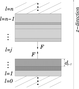
Figure 1: Scheme of the multilayer structure.

For the multilayer structure sketched in Fig. 1 and considered throughout the paper,

$$\varepsilon(\mathbf{r},\omega)=\varepsilon_{l}(\omega)\quad\mbox{for}\quad z_{l}<z<z_{l+1}=z_{l}+d_{l}$$ (20)

($l$ $\!=$ $\!0,\ldots,n$, $z_{0}$ $\!=$ $\!-\infty$, $z_{n+1}$ $\!=$ $\!+\infty$), the Green tensor ${\boldsymbol{\mathit{G}}}_{l}(\mathbf{r},\mathbf{r}^{\prime},\omega)$ in the $l$th layer can be decomposed as

$${\boldsymbol{\mathit{G}}}_{l}(\mathbf{r},\mathbf{r}^{\prime},\omega)={\boldsymbol{\mathit{G}}}_{l}^{\rm bulk}(\mathbf{r},\mathbf{r}^{\prime},\omega)+{\boldsymbol{\mathit{G}}}_{l}^{\rm scat}(\mathbf{r},\mathbf{r}^{\prime},\omega),$$ (21)

where ${\boldsymbol{\mathit{G}}}_{l}^{\rm bulk}$ is the solution emerging from a point-like source current placed in the $l$th layer without any boundaries, and ${\boldsymbol{\mathit{G}}}_{l}^{\rm scat}$ solves the homogeneous version of Eq. (15) so as to make the full Green tensor obey the correct boundary conditions at the surfaces of discontinuity. Since there is no Casimir effect in homogeneous space, the bulk part can safely be dropped (and actually must be dropped) in the stress tensor. The remaining scattering part contains the geometrical data of the problem and is continuous at $\mathbf{r}$ $\!=$ $\!\mathbf{r}^{\prime}$, whereas the bulk part is rather singular there. The scattering part can be constructed as shown in Ref. Tomas . Here, only the case where both spatial arguments are in the same layer is of interest.

II.2 Stress tensor

In order to determine the Casimir force from the stress tensor, we first calculate

$${\boldsymbol{\mathit{T}}}(\mathbf{r,r^{\prime}},t)={\boldsymbol{\mathit{T}}}_{1}(\mathbf{r,r^{\prime}},t)+{\boldsymbol{\mathit{T}}}_{2}(\mathbf{r,r^{\prime}},t)\\[4.30554pt] -\textstyle{\frac{1}{2}}\,{\boldsymbol{\mathit{I}}}\,{\rm Tr}\,[{\boldsymbol{\mathit{T}}}_{1}(\mathbf{r,r^{\prime}},t)+{\boldsymbol{\mathit{T}}}_{2}(\mathbf{r,r^{\prime}},t)],$$ (22)

where

$${\boldsymbol{\mathit{T}}}_{1}\mathbf{(r,r^{\prime}},t)=\bigl{\langle}\hat{\mathbf{D}}(\mathbf{r},t)\otimes\hat{\mathbf{E}}(\mathbf{r^{\prime}},t)\bigr{\rangle}$$ (23)

and

$${\boldsymbol{\mathit{T}}}_{2}\mathbf{(r,r^{\prime}},t)=\bigl{\langle}\hat{\mathbf{B}}(\mathbf{r},t)\otimes\hat{\mathbf{H}}(\mathbf{r^{\prime}},t)\bigr{\rangle}$$ (24)

($\mathbf{r}$ $\!\neq$ $\!\mathbf{r}^{\prime}$). Here, the electromagnetic-field operators are thought of as being expressed in terms of the fundamental fields $\hat{\mathbf{f}}(\mathbf{r},\omega)$ as outlined in Section II.1. To specify the quantum state, we assume thermal equilibrium.

II.2.1 Basic equation

For finite temperatures $T$, we may employ the canonical density operator

$$\hat{\rho}=Z^{-1}e^{-\hat{H}/(k_{\rm B}T)},$$ (25)

where

$$Z={\rm Tr}\,e^{-\hat{H}/(k_{\rm B}T)}.$$ (26)

After some calculation we derive (Appendix A)

$${\boldsymbol{\mathit{T}}}_{1}\mathbf{(r,r^{\prime})}=\mbox{Tr}\,\bigl{[}\hat{\rho}\hat{\mathbf{D}}(\mathbf{r},t)\otimes\hat{\mathbf{E}}(\mathbf{r^{\prime}},t)\bigr{]}$$ (27)

$$=\frac{\hbar}{\pi}\!\int_{0}^{\infty}\!\!d\omega\,\coth\!\left(\!\frac{\hbar\omega}{2k_{\rm B}T}\!\right)\!\frac{\omega^{2}}{c^{2}}\,\Im\!\left[\varepsilon(\mathbf{r,\omega}){\boldsymbol{\mathit{G}}}(\mathbf{r,r^{\prime},\omega})\right],\qquad$$

and

$${\boldsymbol{\mathit{T}}}_{2}\mathbf{(r,r^{\prime})}=\mbox{Tr}\,\bigl{[}\hat{\rho}\hat{\mathbf{B}}(\mathbf{r},t)\otimes\hat{\mathbf{H}}(\mathbf{r^{\prime}},t)\bigr{]}$$ (28)

$$=-\frac{\hbar}{\pi}\!\int_{0}^{\infty}\!\!d\omega\,\coth\!\left(\!\frac{\hbar\omega}{2k_{\rm B}T}\!\right)\boldsymbol{\nabla}\times\Im\!\left[{\boldsymbol{\mathit{G}}}(\mathbf{r,r^{\prime},\omega})\right]\!\times\!\overset{\leftarrow}{\boldsymbol{\nabla}}{{}^{\prime}}.\qquad$$

Here and in the following the time argument $t$ is dropped (because of stationarity). The multilayer Green tensor constructed in terms of generalized Fresnel coefficients is given in Ref. Tomas . The partial translational invariance of the problem (the layers are assumed to have infinite lateral extension) naturally leads to a decomposition of the Green tensor into an angular spectrum of $s$- and $p$-polarized plane waves, whose wave vectors have real components parallel to the multilayer surfaces.

Let the $j$th layer be free space. The Casimir force (per unit area) between the two stacks separated by that layer is then determined by the $zz$-component of the stress tensor obtained from ${\boldsymbol{\mathit{T}}}\mathbf{(r,r^{\prime}})$ in the coincidence limit $\mathbf{r^{\prime}}$ $\!\to$ $\!\mathbf{r}$,

$$T_{zz,j}(\mathbf{r},\mathbf{r})=\lim_{\mathbf{r}^{\prime}\to\mathbf{r}}T_{zz,j}(\mathbf{r},\mathbf{r}^{\prime})$$ (29)

(the index $j$ of a quantity indicates that the quantity refers to the $j$th layer), where – as already mentioned – the (divergent) bulk contribution to the Green tensor must be dropped. Straightforward calculation yields ($\xi_{\sigma}$ $\!=$ $\!\delta_{\sigma p}$ $\!-$ $\!\delta_{\sigma s}$, $\sigma$ $\!=$ $\!s,p$, $M$ $\!=$ $\!\pm$, $N$ $\!=$ $\!\pm$)

$$T_{zz,j}(\mathbf{r,r})=-2\hbar\int_{0}^{\infty}d\omega\,\coth\!\left(\frac{\hbar\omega}{2k_{\rm B}T}\right)\ \times$$ (30)

$$\times\ \Im\biggl{[}\int_{0}^{\infty}\!\!dq\,q\beta_{j}^{2}(q,\omega)\!\!\sum_{M\neq N}\sum_{\sigma}\xi_{\sigma}g_{\sigma j}^{MN}(z,z,q,\omega)\biggr{]}\!.\qquad$$

Here, $\mathbf{q}$ is the transverse component of the wave vector $\mathbf{k}_{j}$ $\!=$ $\!(\mathbf{q},\beta_{j})$, whose $z$-component (‘propagation constant’) $\beta_{j}$ is given by

$$\beta_{j}=\beta_{j}(q,\omega)=\sqrt{\omega^{2}\varepsilon_{j}(\omega)/c^{2}-q^{2}}\,,$$ (31)

and

$$g_{\sigma j}^{MN}(z,z^{\prime},q,\omega)\sim\exp{(M\,i\beta_{j}z)}\exp{(N\,i\beta_{j}z^{\prime})}$$ (32)

is related to the scattering part of the Green tensor as [$\mathbf{r}$ $\!=$ $\!(\boldsymbol{\rho},z)$]

$${\boldsymbol{\mathit{G}}}_{j}^{\rm scat}(\mathbf{r},\mathbf{r^{\prime}},\omega)=\int d^{2}q\,e^{i\mathbf{q}(\boldsymbol{\rho}-\boldsymbol{\rho^{\prime}})}{\boldsymbol{\mathit{G}}}_{j}^{\rm scat}(z,z^{\prime},\mathbf{q},\omega),$$ (33)

$${\boldsymbol{\mathit{G}}}_{j}^{\rm scat}(z,z^{\prime},\mathbf{q},\omega)$$

$$=\sum_{\sigma}\sum_{M,N}g_{\sigma j}^{MN}(z,z^{\prime},q,\omega)\mathbf{{e}}_{\sigma j}^{M}(\mathbf{q})\otimes\mathbf{{e}}_{\sigma j}^{N}(\mathbf{-q}),\quad$$ (34)

with polarization unit vectors

$$\mathbf{{e}}_{sj}^{\pm}(\mathbf{q})=\frac{\mathbf{q}}{q}\times\mathbf{e}_{z},\quad\mathbf{e}_{pj}^{\pm}(\mathbf{q})=\frac{1}{k_{j}}\left(q\mathbf{e}_{z}\mp\beta_{j}\frac{\mathbf{q}}{q}\right)$$ (35)

[$\mathbf{e}_{z}$, unit vector in $z$-direction]. Making use of the explicit form of the Green tensor as given in Tomas , we find after some algebra

$$\beta_{j}^{2}\sum_{M\neq N}\sum_{\sigma}\xi_{\sigma}g_{\sigma j}^{MN}\\ =\frac{i\beta_{j}}{4\pi^{2}}\,e^{2i\beta_{j}d_{j}}\sum_{\sigma}D_{\sigma j}^{-1}r_{j-}^{\sigma}r_{j+}^{\sigma}\cos[\beta_{j}(z-z^{\prime})],$$ (36)

where

$$D_{\sigma j}=D_{\sigma j}(q,\omega)=1-r_{j+}^{\sigma}r_{j-}^{\sigma}e^{2i\beta_{j}d_{j}}$$ (37)

can be thought of as accounting for multiple reflections, with the generalized Fresnel coefficients $r_{j\pm}^{\sigma}$ $\!=$ $\!r_{j\pm}^{\sigma}(q,\omega)$ being the reflection coefficients for $\sigma-$polarized waves at the top ($+$) and bottom ($-$) of the $j$th layer. They can be calculated recursively (for useful recurrence relations, see Appendix B) and in this way expressed in terms of the thicknesses and permittivities of the layers that are actually under consideration. Inserting Eq. (36) into Eq. (30) eventually yields

$$T_{zz,j}=-\frac{\hbar}{2\pi^{2}}\int_{0}^{\infty}d\omega\,\coth\!\left(\frac{\hbar\omega}{2k_{\rm B}T}\right)\ \times\\ \ \times\Re\biggl{(}\int_{0}^{\infty}dq\,q\beta_{j}e^{2i\beta_{j}d_{j}}\sum_{\sigma}D_{\sigma j}^{-1}r_{j-}^{\sigma}r_{j+}^{\sigma}\biggr{)}$$ (38)

($\Re$, real part). Since $T_{zz,j}$ does not depend on the space point in the $j$th layer, the argument $\mathbf{r}$ has been dropped, and Eq. (38) gives the Casimir force (per unit area) that acts on arbitrary multilayered walls.

It should be pointed out that in Eq. (38) nothing is said about the details of stratification of the walls. In fact, any stratified system (whose material properties change only along one direction – here the $z$-direction) admits of separation into an angular spectrum of $s$- and $p$-polarized fields which do never mix BornWolf . This implies that Eq. (38), where the Casimir force is expressed in terms of the reflection coefficients of the walls, is very general and also applies to walls whose permittivity is a (on a macroscopic scale) continuously varying function of $z$. For such walls, however, the reflection coefficients cannot be calculated from simple recurrence relations. In any case, they might be determined experimentally.

When in the zero-temperature limit the overall system is in the ground state $\left|0\right\rangle$, so that $\hat{\mathbf{f}}(\mathbf{r},\omega)\left|0\right\rangle$ $\!=0$ $\forall\>\mathbf{r},\omega$, then the thermal weighting factor $\coth[\hbar\omega/(2k_{\rm B}T)]$ does not appear in Eqs. (27) and (28) and in the equations that follow from them, and thus Eq. (38) changes to Tomaš’ formula TomasCasimir

$$T_{zz,j}=\,-\frac{\hbar}{2\pi^{2}}\!\int_{0}^{\infty}\!\!d\omega\,\ \times$$ (39)

$$\times\ \Re\biggl{(}\int_{0}^{\infty}dq\,q\beta_{j}e^{2i\beta_{j}d_{j}}\sum_{\sigma}D_{\sigma j}^{-1}r_{j-}^{\sigma}r_{j+}^{\sigma}\biggr{)}.$$

II.2.2 Imaginary frequencies

Exploiting the analytical properties of the $\omega$-integrand in Eq. (38) in the upper complex frequency half-plane, we can equivalently rewrite (38) as

$$T_{zz,j}=\frac{\hbar}{2\pi^{2}}\lim_{\eta\to 0+}\Im\Biggl{\{}\int_{0}^{\infty}d\xi\,\biggl{[}\coth\!\left(\frac{\hbar\omega}{2k_{\rm B}T}\right)\ \times\\ \ \times\int_{0}^{\infty}dq\,q\beta_{j}e^{2i\beta_{j}d_{j}}\sum_{\sigma}D_{\sigma j}^{-1}r_{j-}^{\sigma}r_{j+}^{\sigma}\biggr{]}_{\omega=\eta+i\xi}\Biggr{\}},$$ (40)

i.e. the frequency integration is performed on a straight line parallel (and infinitesimally close) to the imaginary frequency axis (for details, see Appendix C). Note that (the small) $\eta$ in Eq. (40) only indicates that the (first-order) poles of the hyperbolic cotangent at the imaginary frequencies

$$\omega_{m}=i\xi_{m}=2im\pi k_{\rm B}T/\hbar$$ (41)

($m$, integer) have to be kept to the left of the integration contour.

In order to further evaluate $T_{zz,j}$ as given by Eq. (40), we first note that in the limit $\eta$ $\!\to$ $\!0+$ the hyperbolic cotangent becomes purely imaginary. Since the permittivity is purely real and positive on the (positive!) imaginary frequency axis (see, e.g., LanLif ), the propagation constant becomes purely imaginary,

$$\beta_{j}(q,\omega=i\xi)=i\kappa_{j}=i\sqrt{\xi^{2}\varepsilon_{j}(i\xi)/c^{2}+q^{2}},$$ (42)

and thus the generalized reflection coefficients become real. Hence, the intervals between the poles (41) do not contribute to the imaginary part in Eq. (40), since the term within the square bracket becomes purely real. Clearly, the same conclusions can also be drawn directly from Eqs. (27) and (28), because the imaginary parts of both the permittivity and the Green tensor vanish at imaginary frequencies. In this way, the $\xi$-integral in Eq. (40) can be given by a residue series according to ($\eta$ $\!\to$ $\!0+$)

$$\Im\biggl{[}\int_{0}^{\infty}d\xi\,f(i\xi)\biggr{]}\\ =2\pi\Im\biggl{[}{\textstyle\frac{1}{2}}\sum_{m=0}^{\infty}\left(1-{\textstyle\frac{1}{2}}\delta_{m0}\right)\mbox{Res}\,f(\omega_{m})\biggr{]},$$ (43)

with the poles from (41). Taking into account that

$$\lim_{\omega\to\omega_{m}}(\omega-\omega_{m})\coth\!\left(\frac{\hbar\omega}{2k_{\rm B}T}\right)\\ =\left[\frac{\partial}{\partial\omega_{m}}\tanh\!\left(\frac{\hbar\omega_{m}}{2k_{\rm B}T}\right)\right]^{-1}=2k_{\rm B}T/\hbar,$$ (44)

[the rest of the integrand is holomorphic; see Appendix C], we eventually derive

$$T_{zz,j}=\frac{k_{\rm B}T}{\pi}\sum_{m=0}^{\infty}\left(1-{\textstyle\frac{1}{2}}\delta_{m0}\right)\ \times\\ \times\ \biggl{[}\int_{0}^{\infty}dq\,q\kappa_{j}e^{-2\kappa_{j}d_{j}}\sum_{\sigma}D_{\sigma j}^{-1}r_{j-}^{\sigma}r_{j+}^{\sigma}\biggr{]}_{\omega=i\xi_{m}}\!,$$ (45)

which may be regarded as a generalization of the popular Lifshitz formula Lifshitz . Note that the zero-frequency term in the Lifshitz formula has been a subject of controversial debate, because the reflection coefficients can be discontinuous at the point $(q$ $\!=$ $\!0$, $\!\omega$ $\!=$ $\!0)$, so that it matters from which direction this point is approached . From the above given derivation of Eq. (45) it follows that first the $q$-integral for a small but non-zero value of $\xi_{0}$ should be calculated and then one can let $\xi_{0}$ $\!\to$ $\!0+$. It should be mentioned that the feasibility of flipping the contour of the frequency integration results from the properties of the Green tensor in the position space, not in the $(\mathbf{q},z)$-space.

To obtain $T_{zz,j}$ in the zero-temperature limit, we may simply set (thanks to $\eta$) $T$ $\!=$ $\!0$ in Eq. (40). The thermal weighting factor thus reduces to unity and we have

$$T_{zz,j}=\frac{\hbar}{2\pi^{2}}\Im\Biggl{\{}\int_{0}^{\infty}\!\!d\xi\!\int_{0}^{\infty}\!\!dq\,q\ \times\\ \times\ \biggl{[}\beta_{j}e^{2i\beta_{j}d_{j}}\!\sum_{\sigma}D_{\sigma j}^{-1}r_{j-}^{\sigma}r_{j+}^{\sigma}\biggr{]}_{\omega=i\xi}\Biggr{\}},$$ (46)

which we may rewrite, on using Eqs. (37) and (42), as

$$T_{zz,j}=\frac{\hbar c}{2\pi^{2}}\!\int_{0}^{\infty}\!\!\frac{d\xi}{c}\!\int_{0}^{\infty}\!\!dq\,q\kappa_{j}e^{-2\kappa_{j}d_{j}}\ \times\\ \times\ \!\biggl{[}\sum_{\sigma}\!\frac{r_{j-}^{\sigma}r_{j+}^{\sigma}}{1-r_{j-}^{\sigma}r_{j+}^{\sigma}e^{-2\kappa_{j}d_{j}}}\!\biggr{]}_{\omega=i\xi}\!.$$ (47)

Of course, Eq. (47) can be obtained by replacing $\sum_{m=0}^{\infty}\cdots$ with $\hbar\,(2\pi k_{\rm B}T)^{-1}\int_{0}^{\infty}d\xi\cdots$ in Eq. (45), since the distance $\Delta\xi_{m}$ $\!=$ $\!2\pi k_{\rm B}T/\hbar$ between neighboring poles [see Eq. (41)] becomes small in the zero-temperature limit, or, alternatively, by flipping the frequency integration contour into the imaginary axis directly in Eq. (39) TomasCasimir .

II.2.3 1D systems

In order to compare the above given macroscopic approach to the Casimir force with the more microscopic approach developed in Kup for one-dimensional systems, we have to perform our calculations for one field component only, e.g.,

$$\underline{\hat{\mathbf{E}}}(\mathbf{r},\omega)={\cal A}^{-1/2}\underline{\hat{E}}(z,\omega)\mathbf{e}_{x}$$ (48)

(${\cal A}$, normalization area; $\mathbf{e}_{x}$, unit vector in $x$-direction). According to the quantization scheme outlined in Sections II.1, the (effectively) scalar electric field strength $\underline{\hat{E}}(z,\omega)$ can be expressed in terms of scalar bosonic basic fields and a scalar Green function. Following the line in Sections II.1 and II.2 and restricting, for simplicity, our attention to the zero-temperature limit, we derive (Appendix D)

$$T_{zz,j}=-\frac{\hbar}{\pi\mathcal{A}}\int_{0}^{\infty}d\omega\,\Re\biggl{[}\frac{\beta_{j}r_{j+}r_{j-}e^{2i\beta_{j}d_{j}}}{D_{j}}\biggr{]},$$ (49)

with $\mathcal{A}$ $\!(\to$ $\!\infty)$ being the normalization area perpendicular to the $z$-direction. Note that instead of Eq. (31) now

$$\beta_{j}=\beta_{j}(\omega)=\frac{\omega}{c}\,\sqrt{\varepsilon_{j}(\omega)}\,$$ (50)

is valid, and the polarization index $\sigma$ can be omitted, since Eq. (48) implies normal incidence and fixed polarization. Equation (49) can formally be obtained from Eq. (39) by making the replacement

$$\frac{1}{4\pi^{2}}\int d^{2}q\quad\mapsto\quad\frac{1}{\mathcal{A}}\sum_{\mathbf{q}}$$ (51)

and keeping only the normally incident waves ($\mathbf{q}$ $\!=$ $\!0$) of fixed ($s$ or $p$) polarization $\sigma$.

In the case of two identical plates (separated by vacuum, i.e. $\varepsilon_{j}$ $\!=$ $\!1$), the reflection coefficients $r_{j+}$ and $r_{j-}$ can be identified with the single-plate reflection coefficient $r_{j}$, i.e. $r_{j\pm}$ $\!=$ $\!r_{j}$. From Eq. (49) it then follows that the Casimir force (per unit area) resulting from the two possible polarizations, $F_{1D}$ $\!=$ $\!2T_{zz,j}$, can be given by

$$F_{1D}=-\frac{2\hbar}{\pi c{\cal A}}\int_{0}^{\infty}d\omega\,\omega\Re\biggl{[}\frac{r_{j}^{2}e^{2i\omega d_{j}/c}}{1-r_{j}^{2}\exp{(2i\omega d_{j}/c)}}\biggr{]},$$ (52)

which corresponds to the result obtained in Kup , if the exact permittivity of the plate material is identified with the model permittivity in Kup . Note that $F_{1D}{\cal A}$ is the total force acting on the normalization area $\mathcal{A}$ $\!(\to$ $\!\infty)$ and not the force per unit area (as erroneously stated in MexicanGuys ).

III Asymptotic distance laws

Let us consider the zero-temperature limit in more detail. In order to evaluate Eq. (47) for the case when $\varepsilon_{j}$ $\!=$ $\!1$ is valid, it is appropriate to change to polar coordinates,

$$\xi/c=\kappa_{j}\cos\phi,\quad q=\kappa_{j}\sin\phi,$$ (53)

and rewrite Eq. (47) as

$$F\equiv T_{zz,j}=\frac{\hbar c}{2\pi^{2}}\int_{0}^{\infty}d\kappa_{j}\,\kappa_{j}^{3}e^{-2\kappa_{j}d_{j}}\int_{0}^{\pi/2}d\phi\,\sin\phi\ \times\\ \times\ \sum_{\sigma}\frac{r_{j-}^{\sigma}r_{j+}^{\sigma}}{1-r_{j-}^{\sigma}r_{j+}^{\sigma}\exp(-2\kappa_{j}d_{j})}\,.$$ (54)

Here and in the following we do not explicitly indicate that $r^{\sigma}_{j\pm}$ $\!=$ $\!r^{\sigma}_{j\pm}(\omega$ $\!=$ $\!ic\kappa_{j}\cos\phi,q$ $\!=$ $\!\kappa_{j}\sin\phi)$. Now, making the $\kappa_{j}$-integral dimensionless by letting

$$u=e^{-2\kappa_{j}d_{j}},\quad du=-2d_{j}\,e^{-2\kappa_{j}d_{j}}d\kappa_{j}$$ (55)

at once extracts the (generic) asymptotic dependence on $d_{j}$ and also yields a finite domain of integration (recommended for numerical computations)

$$F=-F_{0}(d_{j})\ \times\\ \times\ \frac{15}{2\pi^{4}}\!\int_{0+}^{1}\!\!du\,\ln^{3}\!u\int_{0}^{\pi/2}\!\!d\phi\,\sin\phi\sum_{\sigma}\frac{r_{j-}^{\sigma}r_{j+}^{\sigma}}{1-r_{j-}^{\sigma}r_{j+}^{\sigma}u}\,,$$ (56)

where

$$F_{0}(d_{j})=\frac{\hbar c\pi^{2}}{240}\frac{1}{d_{j}^{4}}$$ (57)

is the well-known formula for the force (per unit area) between two perfectly reflecting walls, which was first derived by Casimir Casimir .

III.1 Standard long-distance law

Appendix B shows that the reflection coefficients $r_{j\pm}^{\sigma}$ as functions of $q$ and $\omega$, $r_{j\pm}^{\sigma}$ $\!=$ $\!r_{j\pm}^{\sigma}(q,\omega)$, do not depend on the distance $d_{j}$ between the two reflecting walls. Any dependence on $d_{j}$ of the integral expression in Eq. (56) is therefore a matter of how the reflection coefficients scale with the variable $u$. If $d_{j}$ is large, then only the values of $r_{j\pm}^{\sigma}$ for sufficiently large wavelengths (i.e. small values of both $q$ and $\xi$) can effectively contribute to the integral expression in Eq. (56), whereas the other ones are exponentially suppressed.

Introducing the ‘static’ values of the $\phi$-integrals of $(r_{j+}^{\sigma}r_{j-}^{\sigma})^{m}$,

$$\overline{\left(r_{j+}^{\sigma}r_{j-}^{\sigma}\right)^{m}}=\lim_{\kappa_{j}\to 0+}\int_{0}^{\pi/2}d\phi\,\sin\phi\,\left(r_{j+}^{\sigma}r_{j-}^{\sigma}\right)^{m},$$ (58)

we may evaluate Eq. (54) [or Eq. (56)] in the large-distance limit to obtain

$$F=\frac{F_{0}(d_{j})}{2\zeta(4)}\sum_{\sigma}\overline{{\rm Li}_{4}\!\left({r_{j+}^{\sigma}r_{j-}^{\sigma}}\right)}\qquad(d_{j}\to\infty),$$ (59)

where we have expanded $1/[1$ $\!-$ $\!r_{j+}^{\sigma}r_{j-}^{\sigma}e^{-2\kappa_{j}d_{j}}]$ in powers of $r_{j+}^{\sigma}r_{j-}^{\sigma}e^{-2\kappa_{j}d_{j}}$ and replaced the resulting $\phi$-integrals of powers of $r_{j+}^{\sigma}r_{j-}^{\sigma}$ by their ‘static’ values according to Eq. (58). In Eq. (59), ${\rm Li}_{s}(z)$ $\!=$ $\!\sum_{m=1}^{\infty}z^{m}/m^{s}$ is the polylogarithm function (the series converges for $|z|$ $\!\leq$ $\!1$, $s$ $\!>$ $\!1$), and $\zeta(s)$ $\!=$ $\!\sum_{m=1}^{\infty}m^{-s}$ is the Riemann zeta function [$\zeta(4)$ $\!=$ $\!\pi^{4}/90$]. Clearly, Eq. (59) gives the correct asymptotics only if the ‘static’ polylogarithm does not vanish for the two polarizations (see Section III.2). Using the relation

$${\rm Li}_{s}(|x|\leq 1)\leq\zeta(s)={\rm Li}_{s}(x\to 1-)\qquad(s>1),$$ (60)

from Eq. (59) we see that the asymptotic value of the force is bounded by $F_{0}(d_{j})$. Note that assuming constant reflection coefficients would formally produce the well-known $d_{j}^{-4}$ distance law for arbitrary $d_{j}$. However, this unphysical assumption clearly contradicts the validity of Eq. (54).

Let us briefly discuss the validity of Eq. (59). In order to replace $(r_{j+}^{\sigma}r_{j-}^{\sigma})^{m}$ by $\overline{(r_{j+}^{\sigma}r_{j-}^{\sigma})^{m}}$ according to Eq. (58), the reflection coefficients $r_{j\pm}^{\sigma}$ as functions of $\kappa_{j}$ must be slowly varying on a $\kappa_{j}$-scale of the order of magnitude of $d_{j}^{-1}$. From the structure of the reflection coefficients (Appendix B) it is seen that they depend on $\kappa_{j}$ via the (dependence on frequency of the) permittivities $\varepsilon_{l}$ of the layers and the exponentials $\exp(-2\kappa_{l}d_{l})$. Hence, two conditions must be satisfied. If $\xi_{l}$ is the characteristic frequency scale of variation of $\varepsilon_{l}$ on the imaginary frequency axis, then $\kappa_{j}$ $\!\approx$ $\!d_{j}^{-1}$ must be small compared with $\xi_{l}/c$. Thus, one condition can be given by

$$d_{j}\gg\frac{c}{\xi_{l}}$$ (61)

($l$ $\!\neq$ $\!j$), i.e. the characteristic wavelength $d_{j}$ of the ‘cavity’ formed by the two multilayered walls must be much larger than the characteristic wavelengths of all the wall permittivities . The other condition comes from the requirement that $\kappa_{l}d_{l}$ $\!\ll$ $\!1$ on the relevant $\kappa_{j}$-scale mentioned above. Recalling Eqs. (42) and (53) and the condition (61), we thus arrive at the condition that

$$d_{j}\gg\sqrt{\varepsilon_{l}(i\xi_{l})}\,d_{l}$$ (62)

($l$ $\!\neq$ $\!0,j,n$). Note that in the case of semi-infinite walls considered by Lifshitz Lifshitz only the condition (61) is needed.

III.2 Non-standard long-distance laws

Let us consider, e.g., the case when for small values of $\kappa_{j}$ the relation

$$r_{j\pm}^{\sigma}\simeq\kappa_{j}R_{j\pm}^{\sigma}(\phi)$$ (63)

is valid, with the $R_{j\pm}^{\sigma}$ being bounded functions of $\phi$, so that we may write

$$\frac{r_{j-}^{\sigma}r_{j+}^{\sigma}}{1-r_{j-}^{\sigma}r_{j+}^{\sigma}\exp(-2\kappa_{j}d_{j})}=\kappa_{j}^{2}R_{j-}^{\sigma}R_{j+}^{\sigma}+{\cal O}(\kappa_{j}^{4})$$ (64)

We substitute this expression into Eq. (54) and find that the leading term of the force in the large-distance limit now reads as

$$F = \frac{\hbar c}{2\pi^{2}}\sum_{\sigma}\int_{0}^{\infty}d\kappa_{j}\,\kappa_{j}^{5}e^{-2\kappa_{j}d_{j}}\,\overline{R_{j-}^{\sigma}R_{j+}^{\sigma}}$$ (65)

$$= \frac{15\hbar c}{16\pi^{2}d_{j}^{6}}\sum_{\sigma}\overline{R_{j-}^{\sigma}R_{j+}^{\sigma}}\qquad(d_{j}\to\infty),$$

where

$$\overline{R_{j-}^{\sigma}R_{j+}^{\sigma}}=\lim_{\kappa_{j}\to 0+}\kappa_{j}^{-2}\int_{0}^{\pi/2}d\phi\,\sin\phi\,r_{j-}^{\sigma}r_{j+}^{\sigma}.$$ (66)

Thus, the Casimir force asymptotically behaves like $\sim$ $\!d_{j}^{-6}$. Obviously, other non-standard large-distance laws can also be observed. In particular, when the relation (63) is valid for either $r_{j-}^{\sigma}$ or $r_{j+}^{\sigma}$, then the Casimir force asymptotically behaves like $\sim$ $\!d_{j}^{-5}$.

To be more specific, let us consider the reflection coefficients $r_{j\pm}^{s}$ in more detail. By assuming finite values of $\varepsilon_{j\pm 1}(0)$ and $d_{j\pm 1}$, from Eq. (42) (together with the properties of the permittivity) it follows that ($\varepsilon_{j}$ $\!=$ $\!1$)

$$\frac{1-\sqrt{\varepsilon_{j\pm 1}(0)}}{1+\sqrt{\varepsilon_{j\pm 1}(0)}}\leq\frac{\kappa_{j}-\kappa_{j\pm 1}}{\kappa_{j}+\kappa_{j\pm 1}}\leq 0.$$ (67)

Thus, using Eq. (103) (and the corresponding equation for $r^{s}_{l-}$) and writing

$$r_{l\pm}^{s}=\frac{\displaystyle{\frac{\kappa_{l}-\kappa_{l\pm 1}}{\kappa_{l}+\kappa_{l\pm 1}}}+e^{-2\kappa_{l\pm 1}d_{l\pm 1}}\,r_{(l\pm 1)\pm}^{s}}{1+\displaystyle{\frac{\kappa_{l}-\kappa_{l\pm 1}}{\kappa_{l}+\kappa_{l\pm 1}}}\,e^{-2\kappa_{l\pm 1}d_{l\pm 1}}\,r_{(l\pm 1)\pm}^{s}}\,,$$ (68)

we can establish that for $l$ $\!=$ $\!j$ the inequalities

$$|r_{j\pm}^{s}|\geq\frac{1+\sqrt{\varepsilon_{j\pm 1}(0)}}{2\sqrt{\varepsilon_{j\pm 1}(0)}}\ \times\\ \times\ \left|\left|\frac{\kappa_{j}-\kappa_{j\pm 1}}{\kappa_{j}+\kappa_{j\pm 1}}\right|-e^{-2\kappa_{j\pm 1}d_{j\pm 1}}\bigl{|}r_{(j\pm 1)\pm}^{s}\bigr{|}\right|$$ (69)

and

$$|r_{j\pm}^{s}|\leq{\textstyle\frac{1}{2}}\left[1+\sqrt{\varepsilon_{j\pm 1}(0)}\right]\ \times\\ \times\ \left|\frac{\kappa_{j}-\kappa_{j\pm 1}}{\kappa_{j}+\kappa_{j\pm 1}}+e^{-2\kappa_{j\pm 1}d_{j\pm 1}}r_{(j\pm 1)\pm}^{s}\right|$$ (70)

are valid. The inequality (69) shows that if

$$\lim_{\kappa_{j}\to 0+}|r_{(j\pm 1)\pm}^{s}|\neq\lim_{\kappa_{j}\to 0+}\left|\frac{\kappa_{j}-\kappa_{j\pm 1}}{\kappa_{j}+\kappa_{j\pm 1}}\right|$$ (71)

holds, then (for the chosen values of $\phi$) $r_{j\pm}^{s}$ approaches non-zero values in the limit $\kappa_{j}$ $\!\to$ $\!0+$, making Eq. (63) impossible. Hence, the $d_{j}^{-4}$ law [Eq. (59)] can be expected to hold for large distances. By contrast, if there are single-slab (dielectric) walls, then Eq. (68) yields for $l$ $\!=$ $\!j$ $\!\pm$ $\!1$

$$r_{(j\pm 1)\pm}^{s}=\frac{\kappa_{j\pm 1}-\kappa_{j}}{\kappa_{j\pm 1}+\kappa_{j}}$$ (72)

($r_{(j\pm 2)\pm}^{s}$ $\!=$ $\!0$), and the inequality (70) thus implies that $r_{j\pm}^{s}$ vanishes (uniformly with respect to $\phi$) as $\mathcal{O}(\kappa_{j}d_{j\pm 1})$ in the limit $\kappa_{j}$ $\!\to$ $\!0+$, and a behavior as in Eq. (63) is observed. Note that from Eq. (42) for $\kappa_{j}$ and the corresponding equation for $\kappa_{j+1}$ it follows that the relation

$$\kappa_{j+1}=\kappa_{j}\sqrt{1+[\varepsilon_{j+1}(i\xi)-1]\cos^{2}\phi}$$ (73)

is valid, which reveals that $\kappa_{j+1}$ vanishes with vanishing $\kappa_{j}$. Recall that according to Eq. (53) $\kappa_{j}$ $\!\to$ $\!0+$ entails $\xi$ $\!\to$ $\!0+$. In a similar way it can be shown that (for single-slab walls) the reflection coefficients for $p$-polarization, $r_{j\pm}^{p}$, also vanish uniformly as $\mathcal{O}(\kappa_{j}d_{j\pm 1})$ in the limit $\kappa_{j}$ $\!\to$ $\!0+$. Consequently, when the two walls are single-slab dielectrics, than the $r_{j\pm}^{\sigma}$ behave according to Eq. (63), and hence the $d_{j}^{-6}$-law is observed for large distances, with the functions $R_{j\pm}^{\sigma}(\phi)$ in Eq. (65) being proportional to the respective slab thickness. Clearly, if only one of the two walls consists of a single slab, then the $d_{j}^{-5}$-law may be observed. It should be pointed out that the large-distance asymptotic regime again requires the conditions (61) and (62) to be satisfied.

Let us remark that it is conceivable that other special choices of the walls may produce other than $\sim\!d_{j}^{-4}$, $\sim\!d_{j}^{-5}$, and $\sim\!d_{j}^{-6}$ asymptotic distance dependences of the Casimir force. It may also happen that in the asymptotic expansion of the Casimir force terms $\sim\!d_{j}^{-n}$ with different values of $n$ must be taken into account for not extremely large distances, if the weights of the terms substantially differ from each other.

We finally note that the one-dimensional counterpart of the $d_{j}^{-4}$-law is a $d_{j}^{-2}$-law. It changes to a $d_{j}^{-4}$-law when $r_{j\pm}\simeq\xi R_{j\pm}/c$ holds in the limit $\xi$ $\!\to$ $\!0+$, and it changes to a $d_{j}^{-3}$-law when only one of the reflection coefficients shows this behavior. In particular, two single-slab walls give rise to a $d_{j}^{-4}$-law in place to the standard $d_{j}^{-2}$-law.

III.3 Short-distance law

For short distances, we have to compare the $\kappa_{j}$-scale of variation of the reflection coefficients $r_{j\pm}^{\sigma}$ with the now large scale of variation $d_{j}^{-1}$ of $e^{-2\kappa_{j}d_{j}}$. In particular, assuming $d_{j}$ $\!\ll d_{j\pm 1}$, so that we may let

$$e^{-\kappa_{j\pm 1}d_{j\pm 1}}\approx e^{-\kappa_{j}d_{j\pm 1}}\approx e^{-d_{j\pm 1}/d_{j}}\approx 0,$$ (74)

from Eqs. (103) and (104) (and the corresponding equations for $r^{\sigma}_{l-}$) we see that the reflection coefficients $r_{j\pm}^{\sigma}$ may be approximately replaced by single-interface reflection coefficients according to

$$r^{s}_{j\pm}\approx\frac{\kappa_{j}-\kappa_{j\pm 1}}{\kappa_{j}+\kappa_{j\pm 1}}\,,\quad r^{p}_{j\pm}\approx\frac{\kappa_{j}/\kappa_{j\pm 1}-1/\varepsilon_{j\pm 1}}{\kappa_{j}/\kappa_{j\pm 1}+1/\varepsilon_{j\pm 1}}\,.$$ (75)

Thus, we effectively deal with two semi-infinite walls of permittivities $\varepsilon_{j\pm 1}$, so that Lifshitz’ approximation for short distances can be used Lifshitz :

$$\kappa_{j\pm 1}\approx\kappa_{j}\approx q$$ (76)

and

$$r^{s}_{j\pm}\approx 0,\quad r^{p}_{j\pm}\approx\frac{\varepsilon_{j\pm 1}-1}{\varepsilon_{j\pm 1}+1}\,.$$ (77)

Note that Eqs. (74) and (76) are consistent with each other, and Eq. (76) is valid if

$$\varepsilon_{j\pm 1}(\omega=i\kappa_{j}c)-1\ll 1,$$ (78)

i.e.

$$d_{j}\ll\frac{c}{\Omega_{j\pm 1}}\,,$$ (79)

where the plasma frequencies $\Omega_{l}$ are defined by $\Omega_{l}^{2}$ $\!=$ $\!\lim_{\omega\to\infty}(\omega^{2}\,[1$ $\!-$ $\!\varepsilon_{l}(\omega)])$ Jackson . In this approximation, Eq. (47) takes the well-known form of ($v$ $\!=$ $\!2qd_{j}$)

$$F\approx\frac{\hbar}{16\pi^{2}d_{j}^{3}}\int_{0}^{\infty}d\xi\ \times\\ \times\ \int_{0}^{\infty}dv\,v^{2}\left[\frac{(\varepsilon_{j+1}+1)}{(\varepsilon_{j+1}-1)}\frac{(\varepsilon_{j-1}+1)}{(\varepsilon_{j-1}-1)}e^{v}-1\right]^{-1}.$$ (80)

Let us consider, for simplicity, single-resonance media of Drude-Lorentz type, such that

$$\varepsilon_{j\pm 1}(\omega)=1-\frac{\Omega^{2}}{\omega^{2}+i\gamma_{0}\omega-\omega_{0}^{2}}\,.$$ (81)

For small $\gamma_{0}$, Eq. (80) can then be further evaluated to obtain (Appendix E)

$$F\approx\frac{\hbar}{2\pi d_{j}^{3}}\,\sqrt{\omega_{0}^{2}+\Omega^{2}/2}\,\widetilde{\rm Li}_{2}\!\left[\frac{\Omega^{4}}{64(\omega_{0}^{2}+\Omega^{2}/2)^{2}}\right],$$ (82)

with

$$\widetilde{\rm Li}_{2}(z)=\frac{1}{2}\sum_{m=1}^{\infty}\frac{\Gamma(4m-1)}{[\Gamma(2m)]^{2}}\,\frac{z^{m}}{m^{3}}\,.$$ (83)

IV Numerical results

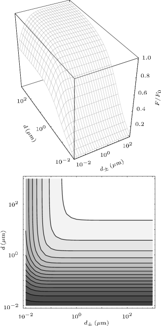
Figure 2: Dependence of the relative Casimir force $F/F_{0}$ between two identical single-slab walls on the thickness $d_{\pm}$ of the walls and the wall separation $d$ (material parameters: $\omega_{0}=1.0\times 10^{9}\,{\rm s}^{-1}=\omega_{\rm LO}$, $\Omega=1.6176\times 10^{16}\,{\rm s}^{-1}\approx 10^{8}\,\omega_{\rm LO}$, $\gamma_{0}=9.7\times 10^{14}\,{\rm s}^{-1}\approx 10^{6}\,\omega_{\rm LO}$).

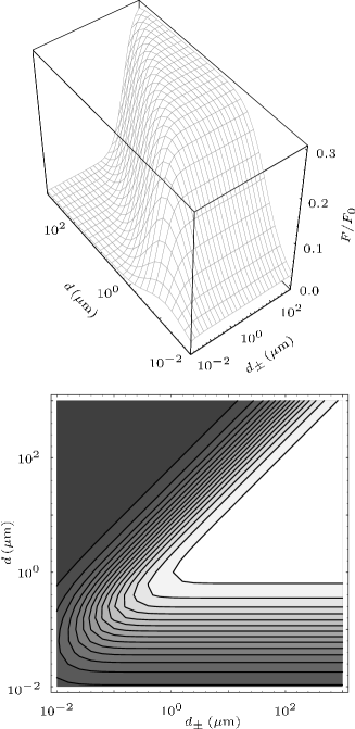
Figure 3: The same as in Fig. 2, but with $\omega_{0}=2.0\times 10^{15}\,{\rm s}^{-1}=\omega_{\rm HI}$, $\Omega=6.536\times 10^{15}\,{\rm s}^{-1}\approx 3\,\omega_{\rm HI}$, and $\gamma_{0}=9.859\times 10^{12}\,{\rm s}^{-1}\approx 0.01\,\omega_{\rm HI}$.

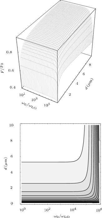
Figure 4: Dependence of the relative Casimir force $F/F_{0}$ between two identical single-slab walls on the resonance frequency $\omega_{0}$ and the wall separation $d$ (wall thickness $d_{\pm}=0.5\,\mu{\rm m}$; material parameters: $\Omega=1.6176\times 10^{16}\,{\rm s}^{-1}\approx 10^{8}\,\omega_{\rm LO}$, $\gamma_{0}=9.7\times 10^{14}\,{\rm s}^{-1}\approx 10^{6}\,\omega_{\rm LO}$).

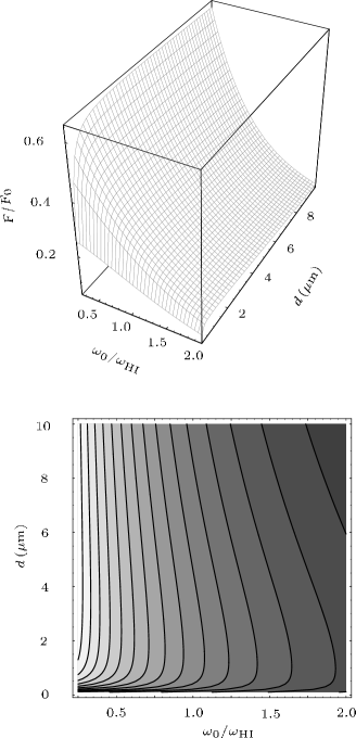
Figure 5: The same as in Fig. 4, but with $d_{\pm}=2.5\,\mu{\rm m}$, $\Omega=6.536\times 10^{15}\,{\rm s}^{-1}\approx 3\,\omega_{\rm HI}$, and $\gamma_{0}=9.859\times 10^{12}\,{\rm s}^{-1}\approx 0.01\,\omega_{\rm HI}$.

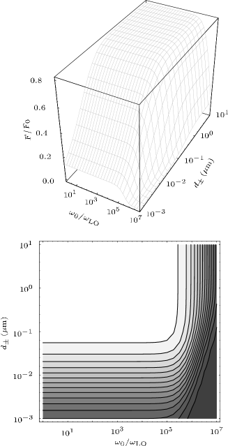
Figure 6: Dependence of the relative Casimir force $F/F_{0}$ between two identical single-slab walls on the resonance frequency $\omega_{0}$ and the wall thickness $d_{\pm}$ (wall separation $d=1\,\mu{\rm m}$; material parameters: $\Omega=1.6176\times 10^{16}\,{\rm s}^{-1}\approx 10^{8}\,\omega_{\rm LO}$, $\gamma_{0}=9.7\times 10^{14}\,{\rm s}^{-1}\approx 10^{6}\,\omega_{\rm LO}$).

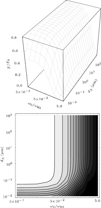
Figure 7: The same as in Fig. 6, but with $d=1\,\mu{\rm m}$, $\Omega=6.536\times 10^{15}\,{\rm s}^{-1}\approx 3\,\omega_{\rm HI}$, and $\gamma_{0}=9.859\times 10^{12}\,{\rm s}^{-1}\approx 0.01\,\omega_{\rm HI}$. The lowest contours are not trustworthy, because of numerical errors.

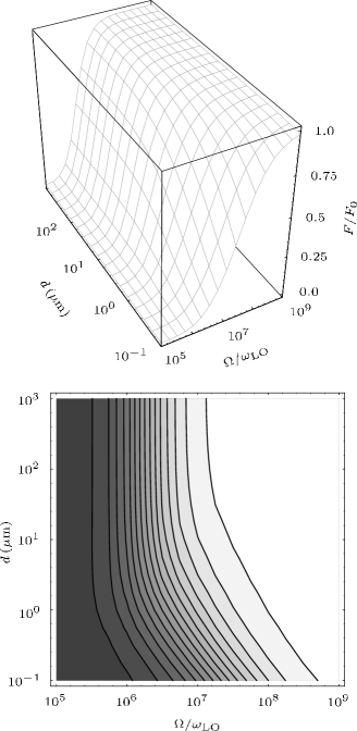
Figure 8: Dependence of the relative Casimir force $F/F_{0}$ between two identical single-slab walls on the plasma frequency $\Omega$ and the wall separation $d$ (wall thickness $d_{\pm}=0.5\,\mu{\rm m}$; material parameters: $\omega_{0}=1.0\times 10^{9}\,{\rm s}^{-1}=\omega_{\rm LO}$, $\gamma_{0}=9.7\times 10^{14}\,{\rm s}^{-1}\approx 10^{6}\,\omega_{\rm LO}$).

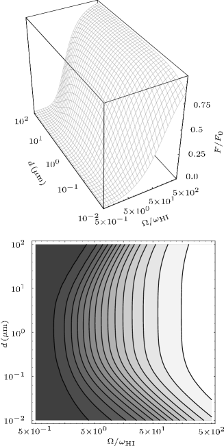
Figure 9: The same as in Fig. 8, but with $d_{\pm}=2.5\,\mu{\rm m}$, $\omega_{0}=2.0\times 10^{15}\,{\rm s}^{-1}=\omega_{\rm HI}$, and $\gamma_{0}=9.859\times 10^{12}\,{\rm s}^{-1}\approx 0.01\,\omega_{\rm HI}$.

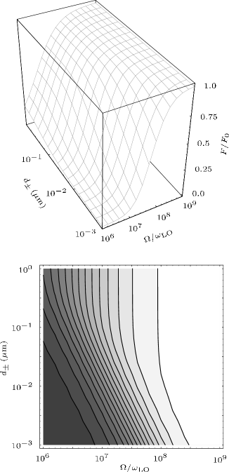
Figure 10: Dependence of the relative Casimir force $F/F_{0}$ between two identical single-slab walls on the plasma frequency $\Omega$ and the wall thickness $d_{\pm}$ (wall separation $d=1\,\mu{\rm m}$; material parameters: $\omega_{0}=1.0\times 10^{9}\,{\rm s}^{-1}=\omega_{\rm LO}$, $\gamma_{0}=9.7\times 10^{14}\,{\rm s}^{-1}\approx 10^{6}\,\omega_{\rm LO}$).

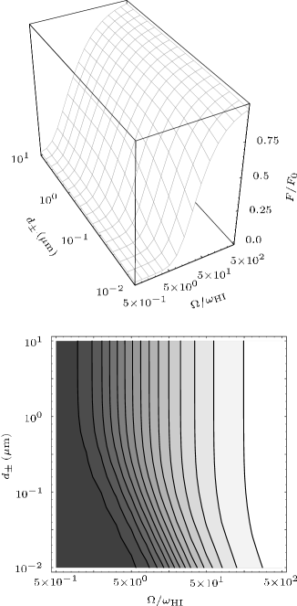
Figure 11: The same as in Fig. 10, but with $d=1\,\mu{\rm m}$, $\omega_{0}=2.0\times 10^{15}\,{\rm s}^{-1}=\omega_{\rm HI}$, and $\gamma_{0}=9.859\times 10^{12}\,{\rm s}^{-1}\approx 0.01\,\omega_{\rm HI}$.

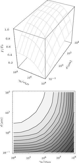
Figure 12: Dependence of the relative Casimir force $F/F_{0}$ between two identical single-slab walls on the absorption parameter $\gamma_{0}$ and the wall separation $d$ (wall thickness $d_{\pm}=0.5\,\mu{\rm m}$; material parameters: $\omega_{0}=1.0\times 10^{9}\,{\rm s}^{-1}=\omega_{\rm LO}$, $\Omega=1.6176\times 10^{16}\,{\rm s}^{-1}\approx 10^{8}\,\omega_{\rm LO}$).

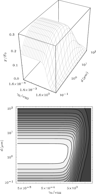
Figure 13: The same as in Fig. 12, but with $d_{\pm}=2.5\,\mu{\rm m}$, $\omega_{0}=2.0\times 10^{15}\,{\rm s}^{-1}=\omega_{\rm HI}$, and $\Omega=6.536\times 10^{15}\,{\rm s}^{-1}\approx 3\,\omega_{\rm HI}$.

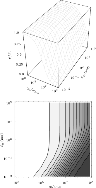
Figure 14: Dependence of the relative Casimir force $F/F_{0}$ between two identical single-slab walls on the absorption parameter $\gamma_{0}$ and the wall thickness $d_{\pm}$ (wall separation $d=10\,\mu{\rm m}$; material parameters: $\omega_{0}=1.0\times 10^{9}\,{\rm s}^{-1}=\omega_{\rm LO}$, $\Omega=1.6176\times 10^{16}\,{\rm s}^{-1}\approx 10^{8}\,\omega_{\rm LO}$).

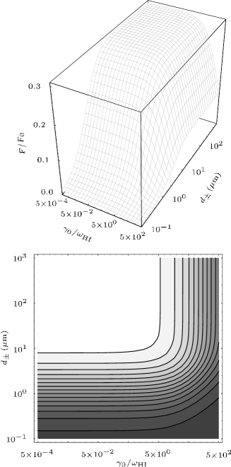
Figure 15: The same as in Fig. 14, but with $d=10\,\mu{\rm m}$, $\omega_{0}=2.0\times 10^{15}\,{\rm s}^{-1}=\omega_{\rm HI}$, and $\Omega=6.536\times 10^{15}\,{\rm s}^{-1}\approx 3\,\omega_{\rm HI}$.

Figure 16: Dependence of the relative Casimir force $F/F_{0}$ between two identical multilayered walls on the wall separation $d$ for various numbers $n$ of identical bilayers (a) L-H and (b) H-L each wall is composed of. The data of the individual layers L and H are respectively $d_{\pm}=0.01\,\mu{\rm m}$, $\omega_{0}=\omega_{\rm LO}=1.0\times 10^{9}\,{\rm s}^{-1}$, $\Omega=1.6176\times 10^{16}\,{\rm s}^{-1}$, $\gamma_{0}=9.7\times 10^{14}\,{\rm s}^{-1}$ and $d_{\pm}=2\,\mu{\rm m}$, $\omega_{0}=\omega_{\rm HI}=2.0\times 10^{15}\,{\rm s}^{-1}$, $\Omega=6.536\times 10^{15}\,{\rm s}^{-1}$, $\gamma_{0}=9.859\times 10^{12}\,{\rm s}^{-1}$.

Figure 17: Detail of Fig. 16.

In order to illustrate the dependence of the Casimir force on the various parameters, we have evaluated Eq. (56) numerically for single-slab walls (Figs. 2 – 15) and a periodic multilayer wall structure (Figs. 16 and 17). The results extend, in a sense, the 1D results given in MexicanGuys to three dimensions. In Figs. 2 – 15, the wall material is characterized by a single-resonance Drude-Lorentz permittivity of the type given in Eq. (81). We have performed the calculations for transverse resonance frequencies $\omega_{0}$ in two qualitatively different frequency domains, namely

$$\omega_{0}\simeq\omega_{\rm LO}=1.0\times 10^{9}\,{\rm s}^{-1}$$ (84)

and

$$\omega_{0}\simeq\omega_{\rm HI}=2.0\times 10^{15}\,{\rm s}^{-1}.$$ (85)

While the higher frequency $\omega_{\rm HI}$ corresponds to dielectric material (such as Si), the lower frequency $\omega_{\rm LO}$ may be regarded as being typical of metal-like material (such as Mg). To allow a comparison with the 1D results in Ref. MexicanGuys , we have performed the numerical calculations for the parameter values used therein. Note that in the contour plots there are always $15$ lines of equal relative force $F/F_{0}$, equidistantly between the highest and the lowest occurring value.

Let us first consider the relative force $F/F_{0}$ between two single-slab walls. The influence of the wall thickness $d_{\pm}$ $\!\equiv\!d_{j\pm 1}$ on the distance law for the two resonance frequencies $\omega_{0}$ $\!=\!\omega_{\rm LO}$ and $\omega_{0}$ $\!=\!\omega_{\rm HI}$, respectively, is shown in Figs. 2 and 3 ($d$ $\!\equiv\!d_{j}$), and the dependence on $\omega_{0}$ of $F/F_{0}$ for chosen $d_{\pm}$ is shown in Figs. 4 and 5. From Figs. 3 and 5 it is seen that (for sufficiently high resonance frequencies) the relative force increases with the distance between the plates, attains a maximum, and eventually decreases with further increasing plate separation. With increasing thickness of the plates the maximum becomes broader and a plateau-like behavior is observed. Figures 2 and 4 reveal that for low resonance frequencies the plateau can become very broad, so that observation of decreasing values of $F/F_{0}$ would require very large distances, at which the force effectively vanishes. Comparing Figs. 2 and 3, we see that the response of the force to a change of the plate thickness is much more sensitive for high resonance frequencies than for low ones. Needless to say that for sufficiently thick plates the force becomes independent of the plate thickness. From Fig. 3 it is seen that the long-distance asymptotic behavior $F$ $\!\sim$ $\!d^{-6}$ [Section III.2] is observed when – in agreement with the condition (62) – the distance between the plates substantially exceeds the plate thickness. A comparison of the 3D results in Figs. 2 and 3 with the 1D results in Fig. 2 in Ref. MexicanGuys shows a quantitatively rather than qualitatively different behavior of the relative force $F/F_{0}$ in the two theories. Clearly, the force itself behaves quite different in the two theories.

Figures 4 and 5 clearly show that increasing the resonance frequency $\omega_{0}$ generally lowers the force. In particular, it is seen that the position of the maximum of the (relative) force is shifted to smaller values of the wall separation when the resonance frequency increases. At the same time, the maximum value decreases and the long-distance asymptotic behavior sets in at smaller distances. The dependence of the force on the resonance frequency is in agreement with the Drude-Lorentz permittivity (81). For chosen plasma frequency $\Omega$ and absorption parameter $\gamma_{0}$, the maximum absolute value of the permittivity decreases with increasing value of $\omega_{0}$, thus reducing the reflection coefficients of the walls. From Figs. 6 and 7 it is seen that increasing the value of the resonance frequency has a similar effect as decreasing the value of the wall thickness. Both a very small plate thickness and a low permittivity can lead to poor plate reflectivity.

The influence of the plasma frequency on the distance law for chosen plate thickness and the two resonance frequencies $\omega_{0}$ $\!=\!\omega_{\rm LO}$ and $\omega_{0}$ $\!=\!\omega_{\rm HI}$ is shown in Figs. 8 and 9, respectively. Figures 10 and 11 illustrate the dependence of the force on the plasma frequency and the thickness of the plates for chosen distance between them. Since the plasma frequency can be regarded as being a measure of the strength of the medium resonance, higher values of the plasma frequency imply higher values of the plate reflectivity and thus higher values of the force, as can be clearly seen from the figures. Moreover, the width of the band-gap featured by the permittivity (81) increases with the plasma frequency, which explains that the interval of large (relative) force also grows with increasing plasma frequency (Fig. 9). In particular, Figs. 10 and 11 show that a high plasma frequency can compensate for a small plate thickness. Note that $\Omega\to\infty$ corresponds to perfectly reflecting plates, whose thickness can then be arbitrarily small.

The effect of material absorption is illustrated in Figs. 12 – 15. The dependence of the distance law on the absorption parameter $\gamma_{0}$ for chosen plate thickness and the two resonance frequencies $\omega_{0}$ $\!=\!\omega_{\rm LO}$ and $\omega_{0}$ $\!=\!\omega_{\rm HI}$, respectively, is shown in Figs. 12 and 13, and Figs. 14 and 15 present the dependence of the force on the absorption parameter and the thickness of the plates for chosen distance between them. As expected, the force is seen to decrease with increasing absorption parameter. The effect is similar to that observed when the resonance frequency is increased. In both cases the maximum absolute value of the permittivity decreases (for chosen plasma frequency), so that the reflection coefficients of the walls diminish. It is worth noting that the force responds more sensitively to a change of $\gamma_{0}/\omega_{0}$ for high resonance frequencies than for low ones. In particular, from Fig. 13 it is seen that in the first case the force is practically not influenced by material absorption as long as $\gamma_{0}/\omega_{0}$ $\!\ll$ $\!1$ is valid, and it effectively reduces to zero when $\gamma_{0}/\omega_{0}$ substantially exceeds unity. Figure 13 also shows that the maximum of the relative force $F/F_{0}$ is shifted to larger values of the distance between the plates when the value of $\gamma_{0}/\omega_{0}$ increases. For low resonance frequencies the ratio $\gamma_{0}/\omega_{0}$ must increase to rather extreme values before the force substantially diminishes, as it is seen from Fig. 12. Note that for a metal ($\omega_{0}$ $\!\to$ $\!0$), $\gamma_{0}$ becomes inversely proportional to the conductivity. Small $\omega_{0}$ and small $\gamma_{0}$, i.e. high conductivity, lead to such a broad plateau of nearly constant (maximum) value of $F/F_{0}$ $\!\approx$ $\!1$ that effectively Casimir’s formula (57) applies.

Let us finally consider the force between two identical multilayered walls composed of identical bilayers, where each bilayer is made of a metal-like and a dielectric-like material (Figs. 16 and 17). For comparison with the 1D results in Ref. MexicanGuys , we have again performed the numerical calculations for the parameter values used therein. From Fig. 16 it is seen that for sufficiently small distances between the walls the force does not depend on the number of bilayers the walls are composed of. In this case, only the inner layers essentially determine the force, which is in full agreement with Eq. (75).

For larger distances between the walls the relative force increases with the number of bilayers. The changes in the curvature of the curves in the figures indicate that (for chosen number of bilayers) the distance law can drastically change several times before the relative forces becomes constant. These changes, which are less pronounced when the inner layers are metal-like ones [Figs. 16(a) and 17(a)], may be regarded as being typical of a 3D theory (cf. Ref. MexicanGuys ).

V Summary

We have studied the Casimir force between dispersing and absorbing multilayered dielectric plates. On the basis of the quantization scheme for the electromagnetic field in causal media as given in Ref. Welsch we have extended the recently derived zero-temperature result TomasCasimir to finite temperatures. The derived formula generalizes Lifshitz’ formula Lifshitz to arbitrary multilayered walls, and application of the 1D version of the theory to single-slab walls yields the results in Ref. Kup .

Restricting our attention to the zero-temperature limit, we have studied the problem of asymptotic distance laws of the Casimir force. We have shown that Lifshitz’ approximation for short distances also applies to multilayered walls and, depending on the wall structure, the distance law can drastically change with increasing wall separation. In particular, for two single-slab walls the Casimir force tends to behave like $d^{-6}$ instead of $d^{-4}$ as the wall separation $d$ goes to infinity.

Assuming permittivities of Drude-Lorentz type, we have finally presented a number of numerical results in order to illustrate the dependence of the zero-temperature Casimir force on various system parameters and to compare with the 1D results recently reported in Ref. MexicanGuys . While in the case of single-slab walls the 3D and the 1D theory yield a qualitatively similar dependence of the relative Casimir force on the wall separation, significant differences (not only for the absolute force but even for the relative force) may be observed for more complicated, multilayered walls.

Appendix A Derivation of Eqs. (27), (28)

It is convenient to discretize the fundamental field variables $\hat{\bf f}({\bf r},\omega)$ so as to work with $\hat{H}=\sum_{\mu,{\bf R}}\hbar\omega_{\mu}\,\hat{\bf f}_{{\bf R},\mu}^{\dagger}\hat{\bf f}_{{\bf R},\mu}$ instead of Eqs. (19) [$(\mathbf{R},\omega_{\mu})$, grid points], and hence with a partition function of the form $Z=\prod_{\mu,{\bf R}}Z^{3}_{{\bf R},\mu}$. From the continuum limit of such a calculation, it then easily follows that

$$\bigl{\langle}\hat{\mathbf{f}}^{\dagger}(\mathbf{r},\omega)\otimes\hat{\mathbf{f}}(\mathbf{r^{\prime}},\omega^{\prime})\bigr{\rangle}\\ ={\boldsymbol{\mathit{\delta}}}(\mathbf{r,r^{\prime}})\delta(\omega-\omega^{\prime})\,\frac{1}{2}\left[\coth\!\left(\frac{{\hbar\omega}}{2k_{\rm B}T}\right)-1\right],$$ (86)

$$\bigl{\langle}\hat{\mathbf{f}}(\mathbf{r},\omega)\otimes\hat{\mathbf{f}}^{\dagger}(\mathbf{r^{\prime}},\omega^{\prime})\bigr{\rangle}\\ ={\boldsymbol{\mathit{\delta}}}(\mathbf{r,r^{\prime}})\delta(\omega-\omega^{\prime})\,\frac{1}{2}\left[\coth\!\left(\frac{{\hbar\omega}}{2k_{\rm B}T}\right)+1\right]$$ (87)

as well as

$$\bigl{\langle}\hat{\mathbf{f}}(\mathbf{r},\omega)\otimes\hat{\mathbf{f}}(\mathbf{r^{\prime}},\omega^{\prime})\bigr{\rangle}=\bigl{\langle}\hat{\mathbf{f}}^{\dagger}(\mathbf{r},\omega)\otimes\hat{\mathbf{f}}^{\dagger}(\mathbf{r^{\prime}},\omega^{\prime})\bigr{\rangle}=0.$$ (88)

Substituting Eq. (1) and the corresponding equation for the displacement field into Eq. (23), we may write, on recalling Eqs. (13), (14), (18) and (88)

$${\boldsymbol{\mathit{T}}}_{1}({\bf r},{\bf r}^{\prime},t)$$ (89)

$$=\int_{0}^{\infty}d\omega\int_{0}^{\infty}d\omega^{\prime}\left[e^{-i(\omega-\omega^{\prime})t}\bigl{\langle}\underline{\hat{\bf D}}({\bf r},\omega)\otimes\underline{\hat{\bf E}}{{}^{\dagger}}({\bf r},\omega)\bigr{\rangle}\right.$$

$$\hskip 43.05542pt\left.+\,e^{i(\omega-\omega^{\prime})t}\bigl{\langle}\underline{\hat{\bf D}}{{}^{\dagger}}({\bf r},\omega)\otimes\underline{\hat{\bf E}}({\bf r},\omega)\bigr{\rangle}\right].$$

Making here explicitly use of Eqs. (13) and (14) and the reciprocity property (16), we obtain

$${\boldsymbol{\mathit{T}}}_{1}({\bf r},{\bf r}^{\prime},t)\\ =\mu_{0}\int_{0}^{\infty}d\omega\int_{0}^{\infty}d\omega^{\prime}\,\omega^{\prime}{{}^{2}}\boldsymbol{\nabla}\times\boldsymbol{\nabla}\times{\boldsymbol{\mathit{K}}}(\mathbf{r,r^{\prime}},\omega,\omega^{\prime},t),$$ (90)

where the tensor-valued function ${\boldsymbol{\mathit{K}}}(\mathbf{r,r^{\prime}},\omega,\omega^{\prime},t)$ is given by

$${\boldsymbol{\mathit{K}}}(\mathbf{r,r^{\prime}},\omega,\omega^{\prime},t)\\ =e^{-i(\omega-\omega^{\prime})t}\bigl{\langle}\bigl{(}{\boldsymbol{\mathit{G}}}\star W{\bf f}\bigr{)}({\bf r},\omega)\otimes\bigl{(}W{\bf f}^{\dagger}\star{\boldsymbol{\mathit{G}}}^{\ast}\bigr{)}({\bf r}^{\prime},\omega^{\prime})\bigr{\rangle}\\ +\,e^{i(\omega-\omega^{\prime})t}\bigl{\langle}\bigl{(}{\boldsymbol{\mathit{G}}}^{\ast}\star W{\bf f}^{\dagger}\bigr{)}({\bf r},\omega)\otimes\bigl{(}W{\bf f}\star{\boldsymbol{\mathit{G}}}\bigr{)}({\bf r}^{\prime},\omega^{\prime})\bigr{\rangle}.$$ (91)

Here, the abbreviating notations

$$W(\mathbf{r},\omega)\equiv\sqrt{\hbar\varepsilon_{0}\varepsilon^{\prime\prime}(\mathbf{r},\omega)/\pi}$$ (92)

and

$$({\boldsymbol{\mathit{G}}}\star\hat{\mathbf{f}})(\mathbf{r},\omega)\equiv\int d^{3}r^{\prime}\,{\boldsymbol{\mathit{G}}}(\mathbf{r},\mathbf{r}^{\prime},\omega)\hat{\mathbf{f}}(\mathbf{r}^{\prime},\omega)$$ (93)

have been used. Applying the integral relation (17) and using Eqs. (86) and (87), from Eqs. (90) and (91) we derive

$${\boldsymbol{\mathit{T}}}_{1}({\bf r},{\bf r}^{\prime})\\ =\frac{\hbar}{\pi}\int_{0}^{\infty}d\omega\,\coth\!\left(\frac{\hbar\omega}{2k_{\rm B}T}\right)\boldsymbol{\nabla}\times\boldsymbol{\nabla}\times\Im[{\boldsymbol{\mathit{G}}}({\bf r},{\bf r}^{\prime},\omega)].$$ (94)

Recalling Eq. (15), we see that Eq. (94) just leads to Eq. (27). The magnetic part ${\boldsymbol{\mathit{T}}}_{2}({\bf r},{\bf r}^{\prime},t)$ [Eq. (24)] can be calculated analogously. In place of Eq. (89) we now have

$${\boldsymbol{\mathit{T}}}_{2}({\bf r},{\bf r}^{\prime},t)$$ (95)

$$=\int_{0}^{\infty}d\omega\int_{0}^{\infty}d\omega^{\prime}\left[e^{-i(\omega-\omega^{\prime})t}\bigl{\langle}\underline{\hat{\bf B}}({\bf r},\omega)\otimes\underline{\hat{\bf H}}{{}^{\dagger}}({\bf r},\omega)\bigr{\rangle}\right.$$

$$\hskip 43.05542pt\left.+\,e^{i(\omega-\omega^{\prime})t}\bigl{\langle}\underline{\hat{\bf B}}{{}^{\dagger}}({\bf r},\omega)\otimes\underline{\hat{\bf H}}({\bf r},\omega)\bigr{\rangle}\right],$$

from which by means of Eqs. (12) and (14) follows that

$${\boldsymbol{\mathit{T}}}_{2}({\bf r},{\bf r}^{\prime},t)\\ =-\mu_{0}\int_{0}^{\infty}d\omega\int_{0}^{\infty}d\omega^{\prime}\,\omega\omega^{\prime}\boldsymbol{\nabla}\times{\boldsymbol{\mathit{K}}}(\mathbf{r,r^{\prime}},\omega,\omega^{\prime},t)\times\overset{\leftarrow}{\boldsymbol{\nabla}}{{}^{\prime}}.$$ (96)

Comparing Eq. (96) with Eqs. (90) and (94), we see that

$${\boldsymbol{\mathit{T}}}_{2}({\bf r},{\bf r}^{\prime})\\ =-\frac{\hbar}{\pi}\int_{0}^{\infty}\!\!d\omega\,\coth\!\left(\frac{\hbar\omega}{2k_{\rm B}T}\right)\boldsymbol{\nabla}\times\Im\!\left[{\boldsymbol{\mathit{G}}}(\mathbf{r,r^{\prime},\omega})\right]\times\!\overset{\leftarrow}{\boldsymbol{\nabla}}{{}^{\prime}}$$ (97)

which is just Eq. (28).

Appendix B Reflection coefficients

Let $\,\,\roarrow{\!\!E}_{l}^{\sigma}(z)$ be the classical (complex) electric field that is observed in the $l$th layer when in a layer $l^{\prime}$ with $l^{\prime}$ $\!<$ $\!l$ an electromagnetic wave (of chosen frequency $\omega$, transverse wave-vector component ${\mathbf{q}}$ and polarization $\sigma$) propagates in $z$-direction (i.e. upwards in Fig. 1). It can be written as

$$\,\roarrow{\!\!E}_{l}^{\sigma}(z)=E_{+l^{\prime}}^{\sigma}{t}_{l^{\prime}/l}^{\sigma}\left[{\bf e}^{+}_{\sigma l}e^{i\beta_{l}z}+e^{2i\beta_{l}d_{l}}r_{l+}^{\sigma}{\bf e}^{-}_{\sigma l}e^{-i\beta_{l}z}\right],$$ (98)

where $E_{+l^{\prime}}^{\sigma}$ is the amplitude of the upwards propagating wave just before the upper boundary of the $l^{\prime}$th layer, ${t}_{l^{\prime}/l}^{\sigma}$ is the transmission coefficient from the $l^{\prime}$th to the $l$th layer ($l^{\prime}$ $\!<$ $\!l$), and $r_{l+}^{\sigma}$ is the reflection coefficient at the upper boundary of the $l$th layer (${\bf e}^{\pm}_{\sigma l}$ according to Eq. (35), $\sigma$ $\!=$ $\!s,p$). Note that we adopt the convention Tomas that $z=0$ denotes the lower boundary in all layers $l$ with $l>0$, and $z=d_{l}$ denotes the upper boundary in all layers $l$ with $l<n$. The transmission and reflection coefficients are determined by the requirement that ${\bf e}_{t}\,\roarrow{\!\!E}_{l}^{\sigma}(z)$ and $({\bf e}_{t}\times\boldsymbol{\nabla})\,\roarrow{\!\!E}_{l}^{\sigma}(z)$ are continuous at the surfaces of discontinuity (${\bf e}_{t}$, tangential unit vector). Applying $\boldsymbol{\nabla}$ in the $(\mathbf{q},z)$-space as $i\mathbf{q}+\mathbf{e}_{z}\partial/\partial z$, straightforward calculation yields the sets of equations

$${t}^{s}_{l^{\prime}/l}e^{i\beta_{l}d_{l}}\bigl{[}1+r^{s}_{l+}\bigr{]}\\ ={t}^{s}_{l^{\prime}/l+1}\bigl{[}1+e^{2i\beta_{l+1}d_{l+1}}r^{s}_{(l+1)+}\bigr{]},$$ (99)

$$\beta_{l}{t}^{s}_{l^{\prime}/l}e^{i\beta_{l}d_{l}}\bigl{[}1-r^{s}_{l+}\bigr{]}\\ =\beta_{l+1}{t}^{s}_{l^{\prime}/l+1}\bigl{[}1-e^{2i\beta_{l+1}d_{l+1}}r^{s}_{(l+1)+}\bigr{]}$$ (100)

[$k_{l}$ $\!=$ $\!\omega\varepsilon_{l}(\omega)^{1/2}/c$ $\!=$ $\!(q^{2}$ $\!+$ $\!\beta_{l}^{2})^{1/2}$] and

$$\frac{\beta_{l}}{k_{l}}t^{p}_{l^{\prime}/l}e^{i\beta_{l}d_{l}}\bigl{[}1-r^{p}_{l+}\bigr{]}\\ =\frac{\beta_{l+1}}{k_{l+1}}\,{t}^{p}_{l^{\prime}/l+1}\bigl{[}1-e^{2i\beta_{l+1}d_{l+1}}r^{p}_{(l+1)+}\bigr{]},$$ (101)

$$k_{l}{t}^{p}_{l^{\prime}/l}e^{i\beta_{l}d_{l}}\bigl{[}1+r^{p}_{l+}\bigr{]}\\ =k_{l+1}{t}^{p}_{l^{\prime}/l+1}\bigl{[}1+e^{2i\beta_{l+1}d_{l+1}}r^{p}_{(l+1)+}\bigr{]}$$ (102)

for $s$ and $p$ polarization, respectively. Eliminating in Eqs. (99 ) – (102) ${t}^{\sigma}_{l^{\prime}/l}e^{i\beta_{l}d_{l}}/{t}^{\sigma}_{l^{\prime}/l+1}$, we derive the recurrences

$$r^{s}_{l+}=\frac{(\beta_{l}/\beta_{l+1}-1)+(\beta_{l}/\beta_{l+1}+1)e^{2i\beta_{l+1}d_{l+1}}r^{s}_{(l+1)+}}{(\beta_{l}/\beta_{l+1}+1)+(\beta_{l}/\beta_{l+1}-1)e^{2i\beta_{l+1}d_{l+1}}r^{s}_{(l+1)+}}$$ (103)

and

$$r^{p}_{l+}=\frac{(\frac{\beta_{l}}{\beta_{l+1}}-\frac{\varepsilon_{l}}{\varepsilon_{l+1}})+(\frac{\beta_{l}}{\beta_{l+1}}+\frac{\varepsilon_{l}}{\varepsilon_{l+1}})e^{2i\beta_{l+1}d_{l+1}}r^{p}_{(l+1)+}}{(\frac{\beta_{l}}{\beta_{l+1}}+\frac{\varepsilon_{l}}{\varepsilon_{l+1}})+(\frac{\beta_{l}}{\beta_{l+1}}-\frac{\varepsilon_{l}}{\varepsilon_{l+1}})e^{2i\beta_{l+1}d_{l+1}}r^{p}_{(l+1)+}},$$ (104)

which terminate at $l$ $\!=$ $\!n$ $\!-$ $\!1$, because of $r^{\sigma}_{n+}$ $\!=$ $\!0$. Note that the $r^{\sigma}_{(n-1)+}$ for the last surface of discontinuity are the well-known single-interface coefficients.

By considering in the same way the solution that emerges in the $l$th layer from a downwards propagating wave in the $l^{\prime}$th layer ($l^{\prime}>l$), analogous recurrences for the coefficients $r^{\sigma}_{l-}$ are derived. They are formally obtained from Eqs. (103) and (104) by making the replacements

$$l\mapsto l,\quad l+1\mapsto l-1$$ (105)

and turning the subscript $+$ of the reflection coefficients into $-$. Because of $r_{0-}^{\sigma}$ $\!=$ $\!0$, they terminate at $l$ $\!=$ $\!1$. From the recurrences it follows that the reflection coefficients are real on the (positive!) imaginary frequency axis and fulfill there the inequality

$$-1\leq r_{l\pm}^{\sigma}\leq 1\qquad(\omega=i\xi).$$ (106)

It should be noted that it is possible to give the $t^{\sigma}_{l^{\prime}/l}$ explicitly once all the $r^{\sigma}_{l\pm}$ have been computed.

Appendix C Integration along the imaginary frequency axis

From Eq. (15) the (exact) Lippmann-Schwinger-type integral equation

$${\boldsymbol{\mathit{G}}}^{\rm scat}(\mathbf{r},\mathbf{r}^{\prime},\omega)\\ =\frac{\omega^{2}}{c^{2}}\int d^{3}s\,{\boldsymbol{\mathit{G}}}^{\rm bulk}(\mathbf{r},\mathbf{s},\omega)\delta\varepsilon(\mathbf{s},\omega){\boldsymbol{\mathit{G}}}(\mathbf{s},\mathbf{r}^{\prime},\omega),$$ (107)

can be derived, where ${\boldsymbol{\mathit{G}}}^{\rm bulk}$ and ${\boldsymbol{\mathit{G}}}^{\rm scat}$ are the bulk and scattering parts of the full Green tensor ${\boldsymbol{\mathit{G}}}$, respectively, and $\delta\varepsilon(\mathbf{r,\omega})$ is the associated deviation of the permittivity from the ‘bulk’ situation. Since any possible Green tensor (such as ${\boldsymbol{\mathit{G}}}$ or ${\boldsymbol{\mathit{G}}}^{\rm bulk}$) has an asymptotic behavior $\mathcal{O}(c^{2}/\omega^{2})$ for $|\omega|\to\infty$ in the upper complex half-plane Welsch , Eq. (107) reveals that $\omega^{2}\varepsilon({\bf r},\omega){\boldsymbol{\mathit{G}}}^{\rm scat}({\bf r},{\bf r}^{\prime},\omega)/c^{2}$ has exactly the same asymptotic behavior as the permittivity difference $\delta\varepsilon(\mathbf{r,\omega})$. We can therefore conclude that frequency integrals of type

$$I=\int_{\mathcal{C}}d\omega\,\frac{\omega^{2}}{c^{2}}\varepsilon(\mathbf{r,\omega}){\boldsymbol{\mathit{G}}}^{\rm scat}(\mathbf{r,r^{\prime},\omega}),$$ (108)

which appear in the zero-temperature versions of Eqs. (27) and (28), are convergent along any contour $\mathcal{C}$ running from the origin (for metals the origin should be excluded, because of the pole at that point) to infinity in a chosen direction of the upper half-plane and yield always the same value, provided that $\delta\varepsilon(\mathbf{r,\omega})$ approaches zero at least as $\mathcal{O}(1/|\omega|^{1+\delta})$ ($\delta$ $\!>$ $\!0$) when $|\omega|$ goes to infinity, which is the case.

Hence, the frequency integration (for zero temperature) in Eqs. (27) and (28) (${\boldsymbol{\mathit{G}}}$ $\!\mapsto$ $\!{\boldsymbol{\mathit{G}}}^{\rm scat}$) can be performed along the positive imaginary axis (instead of the positive real axis) and the imaginary part can be taken after the integration has been performed. In this way, Eq. (39) becomes equivalent to Eq. (46). To include the thermal weighting factor (which behaves like $\omega^{-1}$ for $\omega$ $\!\to$ $\!0$), we first note that integrands of the type which appear in in Eqs. (27) and (28) (${\boldsymbol{\mathit{G}}}$ $\!\mapsto$ $\!{\boldsymbol{\mathit{G}}}^{\rm scat}$) remain perfectly regular at $\omega$ $\!=$ $\!0$, thus

$$\int_{0}^{\infty}d\omega\,\coth\!\left(\frac{\hbar\omega}{2k_{\rm B}T}\right)\Im\,[\ldots]\\ =\lim_{\eta\to 0+}\Im\int_{\eta}^{\infty}d\omega\,\coth\!\left(\frac{\hbar\omega}{2k_{\rm B}T}\right)\ldots.$$ (109)

Since $\coth[\hbar\omega/(2k_{\rm B}T)]$ is holomorphic and bounded for $\Re\omega$ $\!\geq$ $\!\eta$, we now may change the integration path in Eqs. (27) and (28) according to

$$\int_{0}^{\infty}d\omega\,\coth\!\left(\frac{\hbar\omega}{2k_{\rm B}T}\right)\Im\,[\ldots]\\ =\lim_{\eta\to 0+}\Im\int_{\eta}^{\eta+i\infty}d\omega\,\coth\!\left(\frac{\hbar\omega}{2k_{\rm B}T}\right)\cdots,$$ (110)

which then leads to Eq. (40).

Appendix D Derivation of Eq. (49)

The 1D electric field strength $\underline{\hat{\mathbf{E}}}(\mathbf{r},\omega)$ as given in Eq. (48) implies the equations

$$\underline{\hat{\mathbf{B}}}(\mathbf{r},\omega) =\frac{\mathbf{e}_{y}}{i\omega\sqrt{\mathcal{A}}}\,\frac{\partial\underline{\hat{E}}(z,\omega)}{\partial z}\,,$$ (111)

$$\underline{\hat{\mathbf{D}}}(\mathbf{r},\omega) =-\frac{\mathbf{e}_{x}}{\mu_{0}\omega^{2}\sqrt{\mathcal{A}}}\,\frac{\partial^{2}\underline{\hat{E}}(z,\omega)}{\partial z^{2}}$$ (112)

in place of Eqs. (12) and (13), so that Eq. (22) reduces to

$$T_{zz}(\mathbf{r,r^{\prime}},t)=-{\textstyle\frac{1}{2}}\bigl{\langle}\hat{\mathbf{D}}(\mathbf{r},t)\hat{\mathbf{E}}(\mathbf{r^{\prime}},t)+\hat{\mathbf{B}}(\mathbf{r},t)\hat{\mathbf{H}}(\mathbf{r^{\prime}},t)\bigr{\rangle}.$$ (113)

We now proceed further as in the 3D case and substitute the 1D version of Eq. (14) into Eq. (113), where the 1D Green function solves the inhomogeneous wave equation

$$\left[\frac{\partial^{2}}{\partial z^{2}}+\frac{\omega^{2}}{c^{2}}\varepsilon(z,\omega)\right]G(z,z^{\prime},\omega)=-\delta(z-z^{\prime}).$$ (114)

Restricting our attention to the zero-temperature limit, we derive, on applying the 1D versions of Eqs. (16) and (17),

$$\bigl{\langle}0\bigr{|}\underline{\hat{\mathbf{D}}}(\mathbf{r},\omega)\underline{\hat{\mathbf{E}}}{{}^{\dagger}}(\mathbf{r}^{\prime},\omega^{\prime})\bigl{|}0\bigr{\rangle}$$ (115)

$$= -\frac{\mu_{0}\omega^{\prime 2}}{\mathcal{A}}\frac{\partial^{2}}{\partial z^{2}}\bigl{\langle}0\bigr{|}(G\star W\hat{f})(z,\omega)(W\hat{f}^{\dagger}\star G^{\ast})(z^{\prime},\omega^{\prime})\bigl{|}0\bigr{\rangle}$$

$$= -\frac{\hbar}{\pi\mathcal{A}}\,\delta(\omega-\omega^{\prime})\,\frac{\partial^{2}}{\partial z^{2}}\frac{\omega^{2}}{c^{2}}(G\star\varepsilon^{\prime\prime}G^{\ast})(z,z^{\prime},\omega)$$

$$= -\frac{\hbar}{\pi\mathcal{A}}\delta(\omega-\omega^{\prime})\frac{\partial^{2}}{\partial z^{2}}\,\Im\left[G(z,z^{\prime},\omega)\right]$$

$$= \frac{\hbar}{\pi\mathcal{A}}\,\delta(\omega-\omega^{\prime})\,\frac{\omega^{2}}{c^{2}}\,\Im\left[\varepsilon(z,\omega)G(z,z^{\prime},\omega)\right]$$

and

$$\bigl{\langle}0\bigr{|}\underline{\hat{\mathbf{B}}}(\mathbf{r},\omega)\underline{\hat{\mathbf{H}}}{{}^{\dagger}}(\mathbf{r}^{\prime},\omega^{\prime})\bigl{|}0\bigr{\rangle}$$ (116)

$$= \frac{\mu_{0}\omega\omega^{\prime}}{\mathcal{A}}\!\frac{\partial^{2}}{\partial z\partial z^{\prime}}\bigl{\langle}0\bigr{|}(G\star W\hat{f})(z,\omega)(W\hat{f}^{\dagger}\star G^{\ast})(z^{\prime},\omega^{\prime})\bigl{|}0\bigr{\rangle}$$

$$= \frac{\hbar}{\pi\mathcal{A}}\,\delta(\omega-\omega^{\prime})\,\frac{\partial^{2}}{\partial z\partial z^{\prime}}\frac{\omega^{2}}{c^{2}}(G\star\varepsilon^{\prime\prime}G^{\ast})(z,z^{\prime},\omega)$$

$$= \frac{\hbar}{\pi\mathcal{A}}\,\delta(\omega-\omega^{\prime})\,\frac{\partial^{2}}{\partial z\partial z^{\prime}}\,\Im\left[G(z,z^{\prime},\omega)\right]$$

[for $W$ and the $\star$-notation, see Eqs. (92) and (93)]. By Fourier transforming the fields back into the time domain and combining with Eq. (113), we arrive at

$$T_{zz}(\mathbf{r,r^{\prime}})=-\frac{\hbar}{2\pi\mathcal{A}}\int_{0}^{\infty}d\omega\ \times\\ \ \times\Im\left[\frac{\omega^{2}}{c^{2}}\varepsilon(z,\omega)G(z,z^{\prime},\omega)+\frac{\partial^{2}}{\partial z\partial z^{\prime}}G(z,z^{\prime},\omega)\right].$$ (117)

Note that Eq. (117) is valid for an arbitrary $\varepsilon(z,\omega)$.

Let us now specify $\varepsilon(z,\omega)$ according to Eq. (20). The bulk Green function in the $j$th layer reads

$$G_{j}^{\rm bulk}(z,z^{\prime},\omega)=\frac{i}{2\beta_{j}}\,e^{i\beta_{j}|z-z^{\prime}|}$$ (118)

$$\hskip 4.30554pt=g_{j}^{(0)+}e^{i\beta_{j}z}+g_{j}^{(0)-}e^{-i\beta_{j}z}$$

$$\hskip 4.30554pt=\frac{i}{2\beta_{j}}[e^{i\beta_{j}(z-z^{\prime})}\theta(z\!-\!z^{\prime})+e^{-i\beta_{j}(z-z^{\prime})}\theta(z^{\prime}\!-\!z)]\qquad$$

[$\theta(z)$, Heaviside step function], where the propagation constant

$$\beta_{j}=\frac{\omega}{c}\sqrt{\varepsilon_{j}(\omega)}$$ (119)

coincides with the full wave number. The scattering part of the Green function in the $j$th layer

$$G^{\rm scat}_{j}(z,z^{\prime},\omega)=g_{j}^{+}e^{i\beta_{j}z}+g_{j}^{-}e^{-i\beta_{j}z}$$ (120)

is the solution of the homogeneous wave equation, where the matching conditions

$$g_{j}^{+}=r_{j-}\Bigl{(}g_{j}^{(0)-}+g_{j}^{-}\Bigr{)}\quad(z=0<z^{\prime}),$$ (121)

$$g_{j}^{-}e^{-i\beta_{j}d_{j}}=r_{j+}e^{i\beta_{j}d_{j}}\Bigl{(}g_{j}^{(0)+}+g_{j}^{+}\Bigr{)}\quad(z=d_{j}>z^{\prime})$$ (122)

must be satisfied. Thus

$$g_{j}^{\pm}=\frac{r_{j\mp}}{D_{j}}\,e^{i\beta_{j}d_{j}}\Bigl{(}e^{\mp i\beta_{j}d_{j}}g_{j}^{(0)\mp}+e^{i\beta_{j}d_{j}}r_{j\pm}g_{j}^{(0)\pm}\Bigr{)},$$ (123)

$$D_{j}\equiv 1-r_{j+}r_{j-}e^{2i\beta_{j}d_{j}}.$$ (124)

The 1D reflection coefficients $r_{j\pm}$ can be constructed as outlined in Appendix B. Obviously, they are identical to the 3D ones (for $s$-polarization) taken at $\mathbf{q}$ $\!=$ $\!0$ . Combining Eqs. (120) and (123), we find that, on taking $g_{j}^{(0)\pm}$ from Eq. (118),

$$G^{\rm scat}_{j}(z,z^{\prime},\omega)=\frac{ie^{i\beta_{j}d_{j}}}{2\beta_{j}D_{j}}\Bigl{[}r_{j-}e^{-i\beta_{j}d_{j}}e^{i\beta_{j}(z+z^{\prime})}$$

$$\hskip 8.61108pt+\,r_{j-}r_{j+}e^{i\beta_{j}d_{j}}e^{i\beta_{j}(z-z^{\prime})}+r_{j+}e^{i\beta_{j}d_{j}}e^{-i\beta_{j}(z+z^{\prime})}$$

$$\hskip 8.61108pt+\,r_{j+}r_{j-}e^{i\beta_{j}d_{j}}e^{-i\beta_{j}(z-z^{\prime})}\Bigr{]}.$$ (125)

From Eq. (D) it then follows that

$$\frac{\omega^{2}}{c^{2}}\varepsilon(z,\omega)G^{\rm scat}_{j}(z,z^{\prime},\omega)+\frac{\partial^{2}G^{\rm scat}_{j}(z,z^{\prime},\omega)}{\partial z\partial z^{\prime}}\\ =\frac{2i\beta_{j}r_{j+}r_{j-}e^{2i\beta_{j}d_{j}}}{D_{j}}\cos[\beta_{j}(z-z^{\prime})].$$ (126)

Substituting this expression into Eq. (117) [$G(z,z^{\prime},\omega)$ $\!\mapsto$ $\!G^{\rm scat}(z,z^{\prime},\omega)$] and setting $z^{\prime}$ $\!=$ $\!z$, we eventually arrive at Eq. (49).

Appendix E Derivation of Eq. (82)

We first note that Eq. (80) can be rewritten as

$$F\approx\frac{\hbar}{8\pi^{2}d_{j}^{3}}\int_{0}^{\infty}d\xi\,{\rm Li}_{3}\!\left[\frac{(\varepsilon_{j+1}-1)(\varepsilon_{j-1}-1)}{(\varepsilon_{j+1}+1)(\varepsilon_{j-1}+1)}\right].$$ (127)

From Eq. (81) it follows that

$$\frac{\varepsilon_{j\pm 1}(i\xi)-1}{\varepsilon_{j\pm 1}(i\xi)+1}=\frac{1}{1+2[\xi(\xi+\gamma_{0})+\omega_{0}^{2}]/\Omega^{2}}\,.$$ (128)

Substituting this expression into Eq. (127), we obtain [$y$ $\!=$ $\!(\xi$ $\!+$ $\!\gamma_{0}/2)/\Omega$]

$$F\approx\frac{\hbar\Omega}{8\pi^{2}d_{j}^{3}}\sum_{m=1}^{\infty}\frac{I_{m}}{m^{3}}\,,$$ (129)

where

$$I_{m}=\int_{\frac{\gamma_{0}}{2\Omega}}^{\infty}dy\,\left[1+2(y^{2}+\alpha^{2})\right]^{-2m}$$ (130)

and

$$\alpha^{2}\equiv\frac{\omega_{0}^{2}-\gamma_{0}^{2}/4}{\Omega^{2}}.$$ (131)

Under the condition that $\gamma_{0}$ is sufficiently small, so that $\gamma_{0}$ $\!\ll$ $\!2\Omega$ and $\gamma_{0}^{2}/4$ $\!<$ $\!\omega_{0}^{2}$, the integral (130) is approximately given by

$$I_{m}=\frac{1}{2^{2m+1}}\int_{-\infty}^{\infty}\frac{dy}{\left({y^{2}+\alpha^{2}+1/2}\right)^{2m}}\,,$$ (132)

which can be easily evaluated by employing the residue theorem. For this purpose we write

$$\frac{1}{\left(y^{2}+\alpha^{2}+1/2\right)^{2m}}$$ (133)

$$=-\frac{2m}{(2y_{+})^{2m}}\left[\frac{1}{(y-y_{+})(y-y_{-})^{2m-1}}\right.$$

$$\hskip 12.91663pt\left.+\,\frac{1}{(y-y_{-})(y-y_{+})^{2m-1}}\right]+\cdots,$$

where

$$y_{\pm}=\pm i\sqrt{\alpha^{2}+1/2}\,.$$ (134)

We thus derive

$$I_{m}=\frac{\pi}{2^{6m-1}}\frac{\Gamma(4m-1)}{[\Gamma(2m)]^{2}}\,{(\alpha^{2}+1/2)^{1/2-2m}}\,.$$ (135)

Combining Eqs. (129) and (135) eventually yields Eq. (82). Because of

$$\sum_{1}^{\infty}\frac{1}{m^{3}}\int_{0}^{\gamma_{0}/2\Omega}dy\,\left[1+2(y^{2}+\alpha^{2})\right]^{-2m}\\ \leq\frac{\gamma_{0}}{2\Omega}{\rm Li}_{3}\!\left[(\alpha^{2}+1/2)^{-2}/4\right],$$ (136)

the small relative error that results from replacing the lower limit of integration in Eq. (130) by zero can be estimated according to

$$\frac{\delta F}{F}\leq\frac{\gamma_{0}}{\Omega}\,f(\alpha^{2}+1/2),$$ (137)

where [see Eq. (83)]

$$f(x)=\frac{1}{8\pi\sqrt{x}}\,\frac{{\rm Li}_{3}(x^{-2}/4)}{\widetilde{\rm Li}_{2}(x^{-2}/64)}\,.$$ (138)

Note that the factor $f(\alpha^{2}$ $\!+$ $\!1/2)$ is at most of order of unity.

References

• (1) A. Bordag, U. Mohideen, V. M. Mostepanenko, Phys. Rep. 353, 1 (2001).
• (2) S. K. Lamoreaux, Amer. J. Phys., 67, Iss. 10, 850 (1999).
• (3) H.B.G. Casimir, Proc. Kon. Nederl. Akad. Wet. 51, 793 (1948).
• (4) W. Vogel, D.-G. Welsch and S. Wallentowitz, Quantum Optics – An Introduction, 2nd revised and enlarged edition, Wiley, New York, 2001.
• (5) E.M. Lifshitz, Sov. Phys. JETP 2, 73 (1956).
• (6) J. Schwinger, L. L. DeRaad, Jr., K. A. Milton, Ann. Phys. 115, 1 (1978).
• (7) R. Matloob, Phys. Rev. A 64, 042102 (2001).
• (8) D. Kupiszewska, Phys. Rev. A 46, 2286 (1992); see also D. Kupiszewska and J. Mostowski, Phys. Rev. A 41, 4636 (1989).
• (9) R. Esquivel-Sirvent and C. Villarreal, Phys. Rev A 64, 052108 (2001).
• (10) M. S. Tomaš, Phys. Rev. A 66, 052103 (2002).
• (11) N. G. van Kampen, B. R. A. Nijboer and K. Schram, Phys. Lett. 26A, 307 (1968).
• (12) B. W. Ninham, V. A. Parsegian and G. H. Weiss, J. Stat. Phys. 2, 323 (1970); E. Gerlach, Phys. Rev. B 4, 393 (1971); K. Schram, Phys. Lett 43A, 283 (1973); for a more recent application, see, e.g., G. L. Klimchitskaja, U. Mohideen, V. M. Mostepanenko, Phys. Rev. A 61, 062107 (2000).
• (13) M. T. Jaekel, S. Reynaud, J. Phys. I (France) 1, 1395 (1991).
• (14) L. Knöll, S. Scheel, and D.-G. Welsch, QED in dispersing and absorbing dielectric media; in Coherence and Statistic of Photons and Atoms, edited by J. Per̆ina (Wiley, New York, 2001), p. 1.
• (15) M. S. Tomaš, Phys. Rev. A 51, 2545 (1995).
• (16) M. Born and E. Wolf, Principles of Optics (Cambridge University Press, 1997).
• (17) L. D. Landau and E.M. Lifschitz, Lehrbuch der theoretischen Physik Bd. 5 - Statistische Physik (Akademie Verlag Berlin, 1966).
• (18) J. D. Jackson, Klassische Elektrodynamik, 2., verbesserte Auflage (Walter de Gruyter, Berlin, New York, 1983).