Implement Quantum Random Walks with Linear Optics Elements

Abstract

The quantum random walk has drawn special interests because its remarkable features to the classical counterpart could lead to new quantum algorithms. In this paper, we propose a feasible scheme to implement quantum random walks on a line using only linear optics elements. With current single-photon interference technology, the steps that could be experimentally implemented can be extended to very large numbers. We also show that, by decohering the quantum states, our scheme for quantum random walk tends to be classical.

That quantum physics differs from classical physics is due to the quantum coherence, which has been utilized to perform quantum computation such as Shor’s factoring algorithm shor and Grover’s database search algorithm grover . However finding quantum algorithms is very difficult. Recently, several groups have investigated the quantum random walk, with the hope that it might help construct new quantum algorithms aha ; far ; Na ; 7 ; 8 ; Tra ; 10 ; du . Indeed, the first quantum algorithms based on quantum walks with an exponential speedup have been reported al . Further, Travaglione et al. proposed a scheme to implement a discrete-time quantum random walk by an ion trap quantum computer Tra and Dür et al. proposed to use neutral atoms trapped in optical lattices to realized such quantum walks. The first experimental implementation of the quantum random walk algorithm was reported by Du et al. du .

In this paper, we propose a feasible scheme to implement quantum random walks on a line using only linear optics elements. With the defined movement and the dynamic line, we demonstrate that our scheme fulfills all requirements of the quantum random walks. With current single-photon source and its interference technology, our scheme is at the reach of current experiment. The remarkable difference between the quantum and classical random walks could be investigated with a larger number of steps. Also, by decohering the quantum states, our scheme for quantum random walk tends to be classical.

Let us consider a particle performing the discrete-time quantum random walks on a line. Besides the position degrees of freedom, the particle has an additional degree of freedom, namely the “chirality”, which takes value “Left” and “Right”. The walk by such a particle can be described as follows: at every time step, its chirality undergoes the Hadamard transformation and then the particle moves according to its (new) chirality state. In details, the chirality state is denoted by a vector in the Hilbert space spanned by $\left|\text{L}\right\rangle$ (Left) and $\left|\text{R}\right\rangle$ (Right). If the chirality state is $\left|\text{L}\right\rangle$ the particle moves to the left, while if the chirality state is $\left|\text{R}\right\rangle$ the particle moves to the right. Generally, the chirality state might be a superposition of $\left|\text{L}\right\rangle$ and $\left|\text{R}\right\rangle$, this leads the particle moving coherently to both the left and the right. It is this quantum coherence that enables the quantum random walk to remarkably outperform the classical walk.

In order to implement this quantum random walk, the essential idea is to implement the movement depending upon its “chirality” and to perform the Hadamard operation for obtaining further “chirality” for the next step. In our scheme we use the polarization states of photons to represent the “chirality”. We represent the “chirality” state $\left|\text{R}\right\rangle$ by the horizontal polarization photon state $\left|\text{H}\right\rangle$, and $\left|\text{L}\right\rangle$ by vertical polarization state $\left|\text{V}\right\rangle$. The implementation is based on simple linear optical elements, e.g. polarization beam splitters (PBS) and half-wave plates (HWP). When a superposition state passes through a PBS as shown in FIG. 1a, the PBS will direct the photon into two output ports because it transmits only horizontal component and reflects only vertical component. In order to construct the equivalence to the quantum random walk on a line, we could denote the transmission as “Right” side and the reflection as the “Left” side when photons directly pass through the PBS. However,when a superposition state directly passes through a PBS from the “Left” side, it will meet some difficulty since the horizontal component is transmitted and the vertical component is reflected. Thus we need a “modified” PBS (the $\overline{\text{PBS}}$) which transmits the vertical component and reflects the horizontal component. The $\overline{\text{PBS}}$ could be realized by rotating the polarization of the photon by $90^{0}$ with a HWP (let the angle between the HWP axis and horizontal be $45^{0}$) followed by rotating back with two HWP’s after passing through the PBS (R₉₀ as shown in FIG. 1b). After passing through the $\overline{\text{PBS}}$, the horizontal component moves to the “Right” and the vertical component to the “Left”. Also, because there are different components from the two directions, one could conveniently superpose them by one PBS as shown in FIG. 1c. Therefore, with the PBS and the $\overline{\text{PBS}}$ (the modified PBS), we defined the photonic movement depending upon its “chirality”, i.e. polarization degree of freedom of the photons.

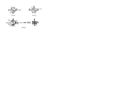
Figure 1: Schematic of the setup to make use of polarization beam splitter (PBS) and half-wave plate (HWP) as the basic elements for implementing the quantum random walk on a line.

During the quantum random walk, one needs to perform a Hadamard operation in each step. This can easily be implemented by rotating the photonic polarization by $45^{0}$ with a HWP (by letting the angle between the HWP axis and horizontal be $22.5^{0}$). After passing the HWP (R₄₅) it will undergo the following Hadamard transformation,

$$\left|\text{H}\right\rangle\rightarrow\frac{1}{\sqrt{2}}\left(\left|\text{H}\right\rangle+\left|\text{V}\right\rangle\right),$$ (1)

$$\left|\text{V}\right\rangle\rightarrow\frac{1}{\sqrt{2}}\left(\left|\text{H}\right\rangle-\left|\text{V}\right\rangle\right).$$ (2)

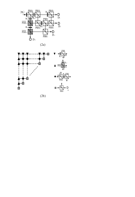
Figure 2: Schematic of the setup to implement quantum random walk on a line with three steps (2a) and the optical network with $N$ steps (2b).

With the defined movement and the Hadamard operation, we can construct the optical network to implement the quantum random walk on a line. Consider the arrangement shown in FIG. 2a, each PBS or $\overline{\text{PBS}}$ denotes an integer point on the line. After the initial polarization photon state $\left|\Psi_{0}\right\rangle$ undergoes a Hadamard transformation and then passes through the PBS₀, the horizontal component moves to the right and the vertical component to the left. Then each $45^{0}$ rotation of the polarization for two components produces the new chirality so that it could proceed the next walk. The transmitted components move to the integer $2$ and $-2$ respectively, and the horizontal component reflected from $\overline{\text{PBS}}_{-1}$ and the vertical component from PBS₁ will overlap at the PBS${}_{0}^{{}^{\prime}}$. Here it should be noted that, in order to let all components move forward and not mix with further input states, we shall introduce a new PBS${}_{0}^{{}^{\prime}}$ to replace the PBS₀, which is equivalent to move the integer $0$ to $0^{\prime}$. The integers $1$, $0^{\prime}$, $-1$ compose a new line, leading to convenient measurement after the random walk, as will be explained later. The state coming out from PBS₁, PBS${}_{0}^{{}^{\prime}}$ and $\overline{\text{PBS}}_{-1}$ further undergoes a Hadamard operation and then performs the next step of the walk. The transmitting components from PBS₂ and $\overline{\text{PBS}}_{-2}$ will move to the position $3$ and $-3$ respectively. The two components reflected from PBS₂ and PBS${}_{0}^{\prime}$ will overlap at PBS${}_{1}^{\prime}$ and the other components reflected from $\overline{\text{PBS}}_{-2}$ and PBS${}_{0}^{\prime}$ will overlap at PBS${}_{-1}^{\prime}$. Introducing PBS${}_{1}^{\prime}$ and PBS${}_{-1}^{\prime}$ to replace the PBS₁ and $\overline{\text{PBS}}_{-1}$ has the same reason as introducing the PBS${}_{0}^{\prime}$. The integers $3$, $1^{\prime}$, $-1$, and $-3$ assemble a new line and one can position four detectors behind them to measure the probability distribution after three steps. By iterating the above steps, we could implement random walk on a line with the unlimited steps in principle by simply adding more PBS’s, $\overline{\text{PBS}}$’s and HWP’s. This optical network for quantum random walk for arbitrary $N$ steps is shown in Fig. 2b.

The essential idea in our scheme is to introduce the dynamic line, which is equivalent to the original line on which the walk is performed. With the moving integer positions we could fulfill all the requirement for the quantum random walk in a line and the scheme provide us a convenient method to measure the distribution after certain steps. Furthermore, it is easily found that the general quantum random walk proposed in Ref. Na can also be implemented in our scheme, by rotating the photonic polarization by arbitrary angle $\theta$ with the HWP (R_θ) rather than $45^{0}$ when performing the Hadamard transformation. Note that in this case the angle between the HWP axis and horizontal should be $\theta/2$.

So far, we have described the quantum random walk on a line. We now discuss how to realize it experimentally. To implement the quantum random walk, the source that produces single photons is demanded. It is available with quantum-dot single photon sources kim ; kur ; lou ; fod or with parametric down conversion kwiat by performing a measurement on one photon. In the quantum random walk, the probability distribution is strongly dependent upon its initial state. The general input $\left|\Psi_{0}\right\rangle=\cos\theta\left|\text{H}\right\rangle+e^{i\varphi}\sin\theta\left|\text{V}\right\rangle$ can be easily obtained by letting single-photon sources pass through two QWP’s and a HWP englert . The key requirement for the experimental realization is to overlap the horizontal component and the vertical one on the PBS in order to utilize the quantum coherence. This could be achieved, such as in the Rome teleportation experiments martini . Finally, the features of the quantum walks could be investigated by positioning detectors behind the PBS’s at the final step. All these requirements have been in the reach of the current technology of linear optics. Also, since the single photon source is very bright, the steps for the quantum random walk are scalable. This is comparative to other scheme such as ion trap Tra or NMR system du with only a few steps. Therefore, with our scheme one can investigate quantum random walks with any initial state for a large number of steps. It should be noted that, whenever taking odd steps or even steps, we need only measure the distribution in the odd positions or in even positions, respectively. But it will not lead to any contradiction because it is obvious that, for either the quantum random walk or the classical one, the probability is zero at even (odd) positions when taking odd (even) steps.

As described by many authors, the remarkably distinguished features between the quantum random walk and the classical one stem from the quantum coherence. However, one could implement the classical random walk by decohering quantum states in our scheme. With slight modification of our scheme, this can be realized by appropriately placing phase shifts more than coherence length of single photon in the optical network, so that the state of the quantum walk decoheres after each step. Therefore, our scheme could be fully used to compare the remarkable features such as the probability distribution and the standard deviation to the classical one for random walk on a line. Further, by changing the phase shift between zero and the coherence length, it is also possible to investigate the decoherence effect in the quantum random walk in experiments.

In conclusion, we have proposed a feasible scheme to implement the quantum random walk on a line with linear optics elements. In the scheme we construct the dynamic line so that we could conveniently measure the probability distribution after certain steps. With nowadays single photon interference technology and highly precise linear optics elements, our scheme are flexible and scalable, and could be implemented experimentally for any initial state with a large number of steps. The experimental realization of quantum random walk also provides us a valuable estimation for quantum computer with linear optics.

This work was supported by the National Natural Science Foundation of China, Chinese Academy of Sciences and the National Fundamental Research Program (Grants No. 2001CB309303 and 2001CB309300).

References

- (1) P. W. Shor, in Proceeding of the 35th Annual Symposium on Foundations of Computer Science (IEEE Computer Society Press, Los Alamitos, CA, 1994), p.124.
- (2) L. K. Grover, Phys. Rev. Lett. 79, 325 (1997).
- (3) Y. Aharonov, L. Davidovich, and N. Zagury, Phys. Rev. A 48, 1687 (1993).
- (4) E. Farhi and S. Gutmann, Phys. Rev. A 58, 915 (1998).
- (5) A. Nayak and A. Vishwanath, quant-ph/0010117.
- (6) A. Ambainis et al., in Proceedings of the 30th annual ACM Symposium on Theory of Computing (Association for Computing Machinery, New York, 2001).
- (7) A. M. Childs et al., quant-ph/0103020; C. Moore and A. Russell, quant-ph/0104037; N. Konno et al., quant-ph/0205065; J. Kempe, quant-ph/0205083; T. Yamasaki et al., quant-ph/205045; E. Bach et al., quant-ph/0207008.
- (8) B. C. Travaglione and G. J. Milburn, Phys. Rev. A 65, 032310 (2002).
- (9) W. Dür et al., Phys. Rev. A 66, 052319 (2002).
- (10) J. Du et al., quant-ph/0203120.
- (11) A. M. Childs et al., quant-ph/0209131; N. Shenvi et al., quant-ph/0210064.
- (12) J. Kim, O. Benson, H. Kan and Y. Yamamoto, Nature (London) 397, 500 (1999).
- (13) C. Kurtsiefer, S. Mayer, P. Zarda, and H. Weinfurter, Phys. Rev. Lett. 85, 290 (2000).
- (14) B. Lounis and W.E. Moerner, Nature (London) 407, 491 (2000).
- (15) C.L. Foden et al., Phys. Rev. A 62, 011803 (2000).
- (16) P.G. Kwiat et al., Phys. Rev. Lett. 75, 4337 (1995).
- (17) B.G. Englert, C. Kurtsiefer, and H. Weinfurter, Phys. Rev. A 63, 032303 (2001).
- (18) D. Boschi et al., Phys. Rev. Lett. 80, 1121 (1998).