Multipartite Entanglement and Hyperdeterminants

Abstract

We classify multipartite entanglement in a unified manner, focusing on a duality between the set of separable states and that of entangled states. Hyperdeterminants, derived from the duality, are natural generalizations of entanglement measures, the concurrence, 3-tangle for 2, 3 qubits respectively. Our approach reveals how inequivalent multipartite entangled classes of pure states constitute a partially ordered structure under local actions, significantly different from a totally ordered one in the bipartite case. Moreover, the generic entangled class of the maximal dimension, given by the nonzero hyperdeterminant, does not include the maximally entangled states in Bell’s inequalities in general (e.g., in the $n\!\geq\!4$ qubits), contrary to the widely known bipartite or 3-qubit cases. It suggests that not only are they never locally interconvertible with the majority of multipartite entangled states, but they would have no grounds for the canonical $n$-partite entangled states. Our classification is also useful for that of mixed states.

I Introduction

The recent development of quantum information science review draws our attention to entanglement, the quantum correlation exhibiting nonlocal (nonseparable) properties, not only as a useful resource but as a renewed fundamental aspect in quantum theory. Since entanglement is supposed to be never strengthened, on average, by local operations and classical communication (LOCC), characterizing it under LOCC is one of our basic interests. Here we classify entanglement of multi-parties, which is less satisfactorily understood than that of two-parties.

When we classify the single copy of multipartite pure states on the Hilbert space ${\mathcal{H}}={\mathbb{C}}^{k_{1}+1}\otimes\cdots\otimes{\mathbb{C}}^{k_{n}+1}$ (precisely, rays on its projective space $M={\mathbb{C}}P^{(k_{1}+1)\cdots(k_{n}+1)-1}$),

$$|\Psi\rangle=\sum_{i_{1},\ldots,i_{n}=0}^{k_{1},\ldots,k_{n}}a_{i_{1},\ldots,i_{n}}|i_{1}\rangle\otimes\cdots\otimes|i_{n}\rangle,$$ (1)

there are many difficulties in applying the techniques, e.g., the Schmidt decomposition, utilized in the bipartite case linden+98 . Still, we can consider a coarser classification by stochastic LOCC (SLOCC) bennett+00 ; dur+00 than LOCC. There we identify two states $|\Psi\rangle$ and $|\Phi\rangle$ that convert to each other back and forth with (maybe different) nonvanishing probabilities, in contrast with LOCC where we identify the states interconvertible deterministically. These states $|\Psi\rangle$ and $|\Phi\rangle$ are supposed to perform the same tasks in quantum information processing, although their probabilities differ. Later, we find that this SLOCC classification is still fine grained to classify the multipartite entanglement. Mathematically, two states belong to the same class under SLOCC if and only if they are converted by an invertible local operation $G$ having a nonzero determinant dur+00 . Thus the SLOCC classification is equivalent to the classification of orbits of the natural action: direct product of general linear groups $GL_{k_{1}+1}({\mathbb{C}})\!\times\!\cdots\!\times\!GL_{k_{n}+1}({\mathbb{C}})$ note1 .

In the bipartite (for simplicity, $k_{1}=k_{2}=k$) case, the SLOCC classification means just classifying the whole states $M$ by the rank of the coefficient matrix $A\!=\!(a_{i_{1},i_{2}})$, also known as the (Schmidt) local rank note2 , because $A$ is transformed as

$$A\;\;\stackrel{{\scriptstyle G}}{{\longrightarrow}}\;\;G^{(1)}\;A\;G^{(2)T},$$ (2)

under an invertible local operation $G=G^{(1)}\otimes G^{(2)}\in GL_{k+1}\times GL_{k+1}$ (the superscript $T$ stands for the transposition) so that its rank is the SLOCC invariant. A set $S_{j}$ of states of the local rank $\leq j$ is a closed subvariety under SLOCC and $S_{j-1}$ is the singular locus of $S_{j}$. This is how the local rank leads to an ”onion” structure acin+01 (mathematically the stratification):

$$M\!=\!S_{k+1}\supset S_{k}\supset\cdots\supset S_{1}\supset S_{0}\!=\!\emptyset,$$ (3)

and $S_{j}\!-\!S_{j-1}\;(j=1,\ldots,k\!+\!1)$ give $k\!+\!1$ classes of entangled states. Now we discuss the relationship between these classes under noninvertible local operations. Since the local rank can decrease by noninvertible local operations, i.e., general LOCC lo+01 , we find that $k\!+\!1$ classes are totally ordered. In particular, the outermost generic set $S_{k+1}\!-\!S_{k}$ is the class of maximally entangled states, for this class can convert to all classes by LOCC but other classes never convert to it. The innermost set $S_{1}(\!=\!S_{1}\!-\!S_{0})$ is that of separable (no-entangled) states. Indeed this class never convert to other classes by LOCC but any other classes can convert to it.

In the 3-qubit case, Dür et al. showed that SLOCC classifies $M$ into finite classes and in particular there exist two inequivalent, Greenberger-Horne-Zeilinger (GHZ) and W, classes of the genuine tripartite entanglement dur+00 . They also pointed out that the SLOCC classification has infinitely many orbits in general (e.g., for $n\geq 4$). In this paper, we classify multipartite entangled states in a unified manner based on hyperdeterminants, and clarify how they are partially ordered. The advantages are three-fold.

1. This classification is equivalent to the SLOCC classification when SLOCC has finitely many orbits. So it naturally includes the widely known bipartite and $3$-qubit cases.

2. In the multipartite case, we need further SLOCC invariants in addition to the local ranks. For example, in the $3$-qubit case dur+00 , the $3$-tangle $\tau$, just the absolute value of the hyperdeterminant (see Eq. (III.1)), is utilized to distinguish GHZ and W classes. This work clarifies why the $3$-tangle $\tau$ appears and how these SLOCC invariants are related to the hyperdeterminant in general.

3. Our classification is also useful to multipartite mixed states. A mixed state $\rho$ can be decomposed as a convex combination of projectors onto pure states. Considering how $\rho$ needs at least the outer class in the onion structure of pure states, we can also classify multipartite mixed states into the totally ordered classes (for details, see the appendix of miyake02 ). We concentrate the pure states here.

The sketch of our idea is as follows. We focus on a duality between the set of separable states and the set of entangled states. The set of completely separable states is the smallest closed subvariety, called Segre variety, $X$, while its dual variety $X^{\vee}$ is the largest closed subvariety which consists of degenerate entangled states (precisely, if $X^{\vee}$ is 1-codimensional). Indeed, in the bipartite ($k_{1}=k_{2}=k$) case, it means that $X$ is the set of states of the local rank $1$, i.e., $X=S_{1}$. On the other hand, $X^{\vee}$ is the set of states where the local rank is not full ($\det A\!=\!0$), i.e., $X^{\vee}=S_{k}$. The duality between the smallest subvariety $X$ and the largest subvariety $X^{\vee}$ holds also for the multipartite case (e.g., see Fig. 3), and the dual variety $X^{\vee}$ is given, in analogy, by the zero hyperdeterminant: ${\rm Det}A\!=\!0$. The outside of $X^{\vee}$, i.e., ${\rm Det}A\!\neq\!0$, is the generic (non degenerate) entangled class, and $|{\rm Det}A|$ is the entanglement measure which represents the amount of generic entanglement. It is also known as the concurrence $C$ hill+97 , $3$-tangle $\tau$ coffman+00 for the $2,3$-qubit pure case, respectively (see Sec.3). It is significant that ${\rm Det}A$ is relatively invariant under SLOCC. In order to obtain other (degenerate) entangled classes, we need to decide the singularities of $X^{\vee}$ as we did in the bipartite case. After this onion-like classification of entangled classes (SLOCC orbits), we characterize the relationship between them under noninvertible local operations. This reveals how multipartite entangled classes are partially ordered, contrary to the bipartite case. We clarify what this structure looks like, as the dimensions $k_{j}\!+\!1$ of subsystems become larger, or as the number $n$ of the parties increases.

Accordingly, the rest of the paper is organized as follows. In Sec.2, the duality between separable states and entangled states is introduced. The hyperdeterminant, associated to this duality, and its singularities lead to the SLOCC-invariant onion-like structure of multipartite entanglement. The characteristics of the hyperdeterminant and its singularities are explained in Sec.3. Classifications of multipartite entangled states are exemplified in Sec.4 so as to reveal how they are ordered under SLOCC. Finally, the conclusion is given in Sec.5.

II Duality between separable states and entangled states

In this section, we find that there is a duality between the set of separable states and that of entangled states. This duality derives the hyperdeterminant our classification is based on.

II.1 Preliminary: Segre variety

To introduce our idea, we first recall the geometry of pure states. In a complex (finite) $k\!+\!1$-dimensional Hilbert space ${\mathcal{H}}({\mathbb{C}}^{k+1})$, let $|\Psi\rangle$ be a (not necessarily normalized) vector given by $k\!+\!1$-tuple of complex amplitudes $x_{j}(j=0,\ldots,k)\in{\mathbb{C}}^{k+1}\!-\!\{0\}$ in a computational basis (i.e., $x_{j}$ are the coefficients in Eq. (1) for $n=1,k_{1}=k$). The physical state in ${\mathcal{H}}({\mathbb{C}}^{k+1})$ is a ray, an equivalence class of vectors up to an overall nonzero complex number. Then the set of rays constitutes the complex projective space ${\mathbb{C}}P^{k}$ and $x:=(x_{0}:\ldots:x_{k})$, considered up to a complex scalar multiple, gives homogeneous coordinates in ${\mathbb{C}}P^{k}$ harris .

For a composite system which consists of ${\mathcal{H}}({\mathbb{C}}^{k_{1}+1})$ and ${\mathcal{H}}({\mathbb{C}}^{k_{2}+1})$, the whole Hilbert space is the tensor product ${\mathcal{H}}({\mathbb{C}}^{k_{1}+1})\otimes{\mathcal{H}}({\mathbb{C}}^{k_{2}+1})$ and the associated projective space is $M={\mathbb{C}}P^{(k_{1}+1)(k_{2}+1)-1}$. A set $X$ of the separable states is the mere Cartesian product ${\mathbb{C}}P^{k_{1}}\times{\mathbb{C}}P^{k_{2}}$, whose dimension $k_{1}\!+\!k_{2}$ is much smaller than that of the whole space $M$, $(k_{1}\!+\!1)(k_{2}\!+\!1)\!-\!1$. This $X$ is a closed, smooth algebraic subvariety (Segre variety) defined by the Segre embedding into ${\mathbb{C}}P^{(k_{1}+1)(k_{2}+1)-1}$ harris ; miyake+01 ,

$${\mathbb{C}}P^{k_{1}}\times{\mathbb{C}}P^{k_{2}}\hookrightarrow{\mathbb{C}}P^{(k_{1}+1)(k_{2}+1)-1}$$

$$\begin{aligned} &\left((x^{(1)}_{0}:\ldots:x^{(1)}_{k_{1}}),(x^{(2)}_{0}:\ldots:x^{(2)}_{k_{2}})\right)\\ &\mapsto\;(x^{(1)}_{0}x^{(2)}_{0}:\ldots:x^{(1)}_{0}x^{(2)}_{k_{2}}:x^{(1)}_{1}x^{(2)}_{0}:\ldots\ldots:x^{(1)}_{k_{1}}x^{(2)}_{k_{2}}).\end{aligned}$$

Denoting homogeneous coordinates in ${\mathbb{C}}P^{(k_{1}+1)(k_{2}+1)-1}$ by $b_{i_{1},i_{2}}\!=\!x^{(1)}_{i_{1}}x^{(2)}_{i_{2}}\;(0\leq i_{j}\leq k_{j})$, we find that the Segre variety $X$ is given by the common zero locus of $k_{1}(k_{1}\!+\!1)k_{2}(k_{2}\!+\!1)/4$ homogeneous polynomials of degree $2$:

$$b_{i_{1},i_{2}}b_{i^{\prime}_{1},i^{\prime}_{2}}-b_{i_{1},i^{\prime}_{2}}b_{i^{\prime}_{1},i_{2}},$$ (4)

where $0\leq i_{1}<i^{\prime}_{1}\leq k_{1},\;0\leq i_{2}<i^{\prime}_{2}\leq k_{2}$. Note that this condition implies that all $2\times 2$ minors of the ”matrix” $B\!=\!(b_{i_{1},i_{2}})$ equal 0; i.e., the rank of $B$ is 1. Thus we have $X=S_{1}$, which agrees with the SLOCC classification by the local rank in the bipartite case.

Now consider the multipartite Cartesian product $X\!=\!{\mathbb{C}}P^{k_{1}}\!\times\!\cdots\!\times\!{\mathbb{C}}P^{k_{n}}$ in the Segre embedding into $M\!=\!{\mathbb{C}}P^{(k_{1}+1)\cdots(k_{n}+1)-1}$. Because this Segre variety $X$ is (the projectivization of) the variety composed of the matrices $B\!=\!(b_{i_{1},\ldots,i_{n}})\!=\!(x^{(1)}_{i_{1}}\cdots x^{(n)}_{i_{n}})$, it gives a set of the completely separable states in ${\mathcal{H}}({\mathbb{C}}^{k_{1}+1})\!\otimes\cdots\otimes\!{\mathcal{H}}({\mathbb{C}}^{k_{n}+1})$. By another Segre embedding, say $X^{\prime}\!=\!{\mathbb{C}}P^{(k_{1}+1)(k_{2}+1)-1}\!\times\!{\mathbb{C}}P^{k_{3}}\!\times\cdots\times\!{\mathbb{C}}P^{k_{n}}$, we also distinguish a set of separable states where only 1st and 2nd parties can be entangled, i.e., when we regard 1st and 2nd parties as one party, an element of this set is completely separable for ”$n\!-\!1$” parties. This is how, also in the multipartite case, we can classify all kinds of separable states, typically lower dimensional sets. Note that, in the multipartite case, this check for the separability is stricter than the check by local ranks note4 .

II.2 Main idea: duality

We rather want to classify entangled states, typically higher dimensional complementary sets of separable states. Our strategy is based on the duality in algebraic geometry harris ; a hyperplane in ${\mathbb{C}}P$ forms the point of a dual projective space ${\mathbb{C}}P^{\ast}$, and conversely every point $p$ of ${\mathbb{C}}P$ is tied to a hyperplane $p^{\vee}$ in ${\mathbb{C}}P^{\ast}$ as the set of all hyperplanes in ${\mathbb{C}}P$ passing through $p$. Let us identify the space of $n$-dimensional matrices with its dual by means of the pairing,

$$F(A,B)=\sum_{i_{1},\ldots,i_{n}=0}^{k_{1},\ldots,k_{n}}a_{i_{1},\ldots,i_{n}}b_{i_{1},\ldots,i_{n}}$$ (5)

(Although in quantum mechanics we take the complex conjugate $a^{\ast}_{i_{1},\ldots,i_{n}}$, compared with $b_{i_{1},\ldots,i_{n}}$, for the product, it does not matter here and we avoid writing the unnecessary superscript.). For a state whose homogeneous coordinates are given by $A$ in ${\mathbb{C}}P^{\ast}_{A}$, $F(A,B)=0$ uniquely determines the hyperplane in ${\mathbb{C}}P_{B}$, which consists of its orthogonal states. Conversely, any hyperplane $F(A,B)=0$ in ${\mathbb{C}}P_{B}$ gives one-to-one correspondence to the point in ${\mathbb{C}}P^{\ast}_{A}$ by its coefficients $A$. This is the duality between points and hyperplanes.

\psfrag{X}{\color[rgb]{0.000,0.500,0.000} {\large$X$}}\psfrag{x}{\normalsize$x$}\psfrag{F}{\color[rgb]{0,0,1}\normalsize$F(A,B)=0$}\psfrag{V}{\color[rgb]{1,0,0} {\large$X^{\vee}$}}\psfrag{D}{\color[rgb]{1,0,0}\normalsize${\rm Det}A=0$ }\psfrag{B}{\normalsize$B$}\psfrag{A}{\normalsize$A$}\includegraphics[width=284.52756pt,clip]{miyake_wadati_fig1.eps}

Figure 1: The duality between the Segre variety $X$ and its dual variety $X^{\vee}$. The set of all hyperplane tangent to $X$ in ${\mathbb{C}}P_{B}$ constitute $X^{\vee}$ in ${\mathbb{C}}P^{\ast}_{A}$.

Remarkably, the projective duality between projective subspaces, like the above example, can be extended to an involutive correspondence between irreducible algebraic subvarieties in ${\mathbb{C}}P$ and ${\mathbb{C}}P^{\ast}$. We define a projectively dual (irreducible) variety $X^{\vee}\subset{\mathbb{C}}P^{\ast}$ as the closure of the set of all hyperplanes tangent to the Segre variety $X$ (see Fig. 1). As sketched in Sec.1, let us observe (and see the reason later) that, for the bipartite case, the variety $S_{k}$ of the degenerate $(k\!+\!1)\times(k\!+\!1)$ matrices $A\!=\!(a_{i_{1},i_{2}})$ is projectively dual to the variety $S_{1}\!=\!X$ of the matrices $B\!=\!(b_{i_{1},i_{2}})\!=\!(x^{(1)}_{i_{1}}x^{(2)}_{i_{2}})$. That is, $S_{k}$ is the dual variety $X^{\vee}$. Following an analogy with a 2-dimensional (bipartite) case, an $n$-dimensional matrix $A\!=\!(a_{i_{1},\ldots,i_{n}})$ is called degenerate if and only if it (precisely, its projectivization) lies in the projectively dual variety $X^{\vee}$ of the Segre variety $X$. In other words, $A$ is degenerate if and only if its orthogonal hyperplane $F(A,B)\!=\!0$ is tangent to $X$ at some nonzero point $x=(x^{(1)},\ldots,x^{(n)})$ (cf. Fig. 1). Analytically, a set of equations,

$$\left\{\mbox{ }\begin{split}&F(A,x)=\sum_{i_{1},\ldots,i_{n}=0}^{k_{1},\ldots,k_{n}}a_{i_{1},\ldots,i_{n}}x^{(1)}_{i_{1}}\cdots x^{(n)}_{i_{n}}=0\\ &\frac{\partial}{\partial x^{(j)}_{i_{j}}}F(A,x)=0\quad\mbox{for all}\;j,i_{j}\end{split}\right.$$ (6)

($j=1,\ldots,n$ and $0\leq i_{j}\leq k_{j}$), has at least a nontrivial solution $x\!=\!(x^{(1)},\ldots,x^{(n)})$ of every $x^{(j)}\!\neq\!0$, and then $x$ is called a critical point. The above condition is also equivalent to saying that the kernel ${\rm ker}F$ of $F(A,x)$ is not empty, where ${\rm ker}F$ is the set of points $x=(x^{(1)},\ldots,x^{(n)})\in X$ such that, in every $j_{0}=1,\ldots,n$,

$$F\mbox{$($}A,(x^{(1)},\ldots,x^{(j_{0}-1)},z^{(j_{0})},x^{(j_{0}+1)},\ldots,x^{(n)})\mbox{$)$}=0,$$ (7)

for the arbitrary $z^{(j_{0})}$.

In the case of $n\!=\!2$, the condition for Eqs.(LABEL:eq:critical) coincides with the usual notion of degeneracy and means that $A\!=\!(a_{i_{1},i_{2}})$ does not have the full rank. It shows that $X^{\vee}$ is nothing but $S_{k}$. In particular, $X^{\vee}$, defined by this condition, is of codimension 1 and is given by the ordinary determinant $\det A\!=\!0$, if and only if $A$ is a square $(k_{1}\!=\!k_{2}\!=\!k)$ matrix. In the $n$-dimensional case, if $X^{\vee}$ is a hypersurface (of codimension 1), it is given by the zero locus of a unique (up to sign) irreducible homogeneous polynomial over ${\mathbb{Z}}$ of $a_{i_{1},\ldots,i_{n}}$. This polynomial is the hyperdeterminant introduced by Cayley cayley and is denoted by ${\rm Det}A$. As usual, if $X^{\vee}$ is not a hypersurface, we set ${\rm Det}A$ to be 1.

Remember that, in the bipartite case, we classify the states $\in S_{k+1}\!-\!S_{k}\!=\!M\!-\!X^{\vee}$ as the generic entangled states, the states $\in S_{k}\!-\!S_{k-1}\!=\!X^{\vee}\!-\!X^{\vee}_{\rm sing}$ as the next generic entangled states, and so on. Likewise, we aim to classify the multipartite entangled states into the onion structure by the dual variety $X^{\vee}$ (${\rm Det}A\!=\!0$), its singular locus $X^{\vee}_{\rm sing}$ and so on, i.e., by every closed subvariety.

III Hyperdeterminant and its singularities

In order to classify multipartite entanglement into the SLOCC-invariant onion structure, we explore the dual variety $X^{\vee}$ (zero hyperdeterminant) and its singular locus in this section.

III.1 Hyperdeterminant

We utilize the hyperdeterminant, the generalized determinant for higher dimensional matrices by Gelfand et al. gelfand+92 ; gelfand+94 . Its absolute value is also known as an entanglement measure, the concurrence $C$ hill+97 , 3-tangle $\tau$ coffman+00 respectively, for the 2,3-qubit pure case.

$$C =2|{\rm Det}A_{2}|=2|\det A|=2|a_{00}a_{11}-a_{01}a_{10}|,$$ (8)

$$\tau =4|{\rm Det}A_{3}|$$

$$=4|a_{000}^{2}a_{111}^{2}+a_{001}^{2}a_{110}^{2}+a_{010}^{2}a_{101}^{2}+a_{100}^{2}a_{011}^{2}-2(a_{000}a_{001}a_{110}a_{111}+a_{000}a_{010}a_{101}a_{111}$$

$$\quad\mbox{}+a_{000}a_{100}a_{011}a_{111}+a_{001}a_{010}a_{101}a_{110}+a_{001}a_{100}a_{011}a_{110}+a_{010}a_{100}a_{011}a_{101})$$

$$\quad\mbox{}+4(a_{000}a_{011}a_{101}a_{110}+a_{001}a_{010}a_{100}a_{111})|.$$ (9)

The following useful facts are found in gelfand+94 . Without loss of generality, we assume that $k_{1}\!\geq\!k_{2}\!\geq\!\cdots\!\geq\!k_{n}\!\geq\!1$. The $n$-dimensional hyperdeterminant ${\rm Det}A$ of format $(k_{1}\!+\!1)\!\times\!\cdots\!\times\!(k_{n}\!+\!1)$ exists, i.e., $X^{\vee}$ is a hypersurface, if and only if a ”polygon inequality” $k_{1}\!\leq\!k_{2}+\cdots\!+\!k_{n}$ is satisfied. For $n\!=\!2$, this condition is reduced to $k_{1}\!=\!k_{2}$ as desired, and ${\rm Det}A$ coincides with $\det A$. The matrix format is called boundary if $k_{1}\!=\!k_{2}\!+\cdots+\!k_{n}$ and interior if $k_{1}\!<\!k_{2}\!+\cdots+\!k_{n}$. Note that (i) The boundary format includes the ”bipartite cut” between 1st parties and the others so that it is mathematically tractable. (ii) The interior format includes the $n\!\geq\!3$-qubit case. We treat hereafter the format where the polygon inequality holds and $X^{\vee}$ is the largest closed subvariety, defined by the hypersurface ${\rm Det}A=0$.

${\rm Det}A$ is relatively invariant (invariant up to constant) under the action of $GL_{k_{1}+1}({\mathbb{C}})\times\cdots\times GL_{k_{n}+1}({\mathbb{C}})$. In particular, interchanging two parallel slices (submatrices with some fixed directions) leaves ${\rm Det}A$ invariant up to sign, and ${\rm Det}A$ is a homogeneous polynomial in the entries of each slice. Since it is ensured that $X^{\vee}$, $X^{\vee}_{\rm sing}$ and further singularities are invariant under SLOCC, our classification is equivalent to or coarser than the SLOCC classification. Later, we see that the former and the latter correspond to the case where SLOCC gives finitely and infinitely many classes, respectively.

III.2 Schläfli’s construction

It would be not easy to calculate ${\rm Det}A$ directly by its definition that Eqs.(LABEL:eq:critical) have at least one solution. Still, the Schläfli’s method enables us to construct ${\rm Det}A_{n}$ of format $2^{n}$ ($n$ qubits) by induction on $n$ gelfand+92 ; gelfand+94 ; schlafli .

For $n\!=\!2$, by definition ${\rm Det}A_{2}\!=\!\det A\!=\!a_{00}a_{11}\!-\!a_{01}a_{10}$. Suppose ${\rm Det}A_{n}$, whose degree of homogeneity is $l$, is given. Associating an $n\!+\!1$-dimensional matrix $A\!=\!(a_{i_{0},i_{1},\ldots,i_{n}})$ ($i_{j}\!=\!0,1$) to a family of $n$-dimensional matrices $\widetilde{A}(x)\!=\!\left(\sum_{i_{0}}a_{i_{0},i_{1},\cdots,i_{n}}x_{i_{0}}\right)$ which linearly depend on the auxiliary variable $x_{i_{0}}$, we have ${\rm Det}\widetilde{A}(x)_{n}$. Due to Theorem 4.1, 4.2 of gelfand+94 , the discriminant $\Delta$ of ${\rm Det}\widetilde{A}(x)_{n}$ gives ${\rm Det}A_{n+1}$ with an extra factor $R_{n}$. The Sylvester formula of the discriminant $\Delta$ for binary forms enables us to write ${\rm Det}A_{n+1}$ in terms of the determinant of order $2l\!-\!1$;

$${\rm Det}A_{n+1}=\frac{\Delta({\rm Det}\widetilde{A}(x)_{n})}{R_{n}}=\frac{1}{R_{n}c_{l}}\left|\begin{array}[]{cccccccc}c_{0}&c_{1}&\cdots&c_{l-2}&c_{l-1}&c_{l}&\cdots&0\\ 0&c_{0}&\cdots&\cdots&c_{l-2}&c_{l-1}&\cdots&0\\ \vdots&&\ddots&&\vdots&&\ddots&\vdots\\ 0&0&\cdots&c_{0}&c_{1}&\cdots&\cdots&c_{l}\\ 1c_{1}&2c_{2}&\cdots&\cdots&lc_{l}&0&\cdots&0\\ \vdots&&\ddots&&\vdots&&\ddots&\vdots\\ 0&0&\cdots&0&1c_{1}&2c_{2}&\cdots&lc_{l}\\ \end{array}\right|,$$ (10)

where each $c_{j}$ is the coefficient of $x_{0}^{l-j}x_{1}^{j}$ in ${\rm Det}\widetilde{A}(x)_{n}$, i.e., $c_{j}=\frac{1}{(l-j)!\;j!}\frac{\partial^{l}}{\partial x_{0}^{l-j}\partial x_{1}^{j}}{\rm Det}\widetilde{A}(x)_{n}$.

Note that because for $n\!=\!2,3$, the extra factor $R_{n}$ is just a nonzero constant, ${\rm Det}A_{3,4}$ for the $3,4$ qubits is readily calculated respectively. It would be instructive to check that ${\rm Det}A_{3}$ in Eq.(III.1) is obtained in this way. On the other hand, for $n\!\geq\!4$, $R_{n}$ is the Chow form (related resultant) of irreducible components of the singular locus $X^{\vee}_{\rm sing}$. These are due to the fact that $X^{\vee}_{\rm sing}$ has codimension $2$ in $M$ for any formats of the dimension $n\!\geq\!3$ except for the format $2^{3}$ ($3$-qubit case), which was conjectured in gelfand+92 and was proved in weyman+96 . So we have to explore $X^{\vee}_{\rm sing}$ not only to classify entangled states in the $n$ qubits, but to calculate ${\rm Det}A_{n+1}$ inductively. Although ${\rm Det}A_{n\geq 5}$ has yet to be written explicitly, only its degree $l$ of homogeneity is known (in Corollary 2.10 of gelfand+94 ) to grow very fast as $2,4,24,128,880,6816,60032,589312,6384384$ for $n=2,3,\ldots,10$. It can be said that this monstrous degree reflects the richness of multipartite entanglement, compared with the linear scaling ($\propto k$) of the degree along the dimensional direction for the bipartite $(k\!+\!1)\times(k\!+\!1)$ case.

III.3 Singularities of the hyperdeterminant

We describe the singular locus of the dual variety $X^{\vee}$. The technical details are given in weyman+96 . It is known that, for the boundary format, the next largest closed subvariety $X^{\vee}_{\rm sing}$ is always an irreducible hypersurface in $X^{\vee}$; in contrast, for the interior one, $X^{\vee}_{\rm sing}$ has generally two closed irreducible components of codimension 1 in $X^{\vee}$, node $X^{\vee}_{\rm node}$ and cusp $X^{\vee}_{\rm cusp}$ type singularities. The rest of this subsection can be skipped for the first reading. It is also illustrated for the 3-qubit case in the appendix of miyake02 .

\psfrag{X}{\large{$X$}}\psfrag{V}{\large{$X^{\vee}$}}\includegraphics[clip]{miyake_wadati_fig2.eps}

Figure 2: Two types of singularities of $X^{\vee}$. $X^{\vee}_{\rm node}$ corresponds to the bitangent of $X$, where both tangencies are of the first order. $X^{\vee}_{\rm cusp}$ corresponds to the tangent at an inflection point of $X$, where its tangency is of the second order.

First, $X^{\vee}_{\rm node}$ is the closure of the set of hyperplanes tangent to the Segre variety $X$ at more than one points (cf. Fig. 2). $X^{\vee}_{\rm node}$ can be composed of closed irreducible subvarieties $X^{\vee}_{\rm node}(J)$ labeled by the subset $J\!\subset\!\{1,\ldots,n\},$ including $\emptyset$. Indicating that two solutions $x\!=\!(x^{(1)},\ldots,x^{(j)},\ldots,x^{(n)})$ of Eq.(LABEL:eq:critical) coincide for $j\!\in\!J$, the label $J$ distinguishes the pattern in these solutions. In order to rewrite $X^{\vee}_{\rm node}(J)$, let us pick up a point $x^{o}(J)$ such that its homogeneous coordinates $x^{(j)}_{i_{j}}=\delta_{i_{j},0}$ for $j\!\in\!J$ and $\delta_{i_{j},k_{j}}$ for $j\!\notin\!J$. It is convenient to label the positions of $1$ in each $x^{(j)}$ by a multi-index $[i_{1},\ldots,i_{n}]$. For example, $x^{o}(1)$ is labeled by $[0,k_{2},\ldots,k_{n}]$ and $x^{o}(1,\ldots,n)$ is just written by $x^{o}$. When $X^{\vee}$ is the hyperplane tangent to $X$ at $x^{o}(J)$, its ”$x^{o}(J)$-section” $X^{\vee}|_{x^{o}(J)}$ is given as

$$X^{\vee}|_{x^{o}(J)}=\left\{A\;\left|\;\mbox{all $a_{i^{\prime}_{1},\ldots,i^{\prime}_{n}}\!=\!0$ s.t. }\begin{array}[]{l}\mbox{$[i^{\prime}_{1},\ldots,i^{\prime}_{n}]$ differs from $[i_{1},\ldots,i_{n}]$}\\ \mbox{of $x^{o}(J)$ in at most one index}\end{array}\right.\right\},$$ (11)

in order that Eqs.(LABEL:eq:critical) have the nontrivial solution $x^{o}(J)$. Then in terms of the hyperplane bitangent to $X$ at $x^{o}$ and $x^{o}(J)$, we can define $X^{\vee}_{\rm node}(J)$ as

$$X^{\vee}_{\rm node}(J)=\overline{(X^{\vee}|_{x^{o}}\cap X^{\vee}|_{x^{o}(J)})\cdot G},$$ (12)

where $G\!=\!GL_{k_{1}+1}\!\times\!\cdots\!\times\!GL_{k_{n}+1}$ acts $M$ on from the right and the bar stands for the closure.

Second, $X^{\vee}_{\rm cusp}$ is the set of hyperplanes having a critical point which is not a simple quadratic singularity (cf. Fig. 2). Precisely, the quadric part of $F(A,x)$ at $x^{o}$ is a matrix $y_{(j,i_{j}),(j^{\prime},i_{j^{\prime}})}\!=\!(\partial^{2}/\partial x_{i_{j}}^{(j)}\partial x_{i_{j^{\prime}}}^{(j^{\prime})})F(A,x^{o})$, where the pairs $(j,i_{j}),\>(j^{\prime},i_{j^{\prime}})\>(1\!\leq\!i_{j}\!\leq\!k_{j},\>1\!\leq\!i_{j^{\prime}}\!\leq\!k_{j^{\prime}})$ are the row, column index respectively. Denoting by $X^{\vee}_{\rm cusp}|_{x^{o}}$ the variety of the Hessian $\det y\!=\!0$ in the $x^{o}$-section $X^{\vee}|_{x^{o}}$ of Eq. (11), we can define $X^{\vee}_{\rm cusp}$ as

$$X^{\vee}_{\rm cusp}=X^{\vee}_{\rm cusp}|_{x^{o}}\cdot G.$$ (13)

This $X^{\vee}_{\rm cusp}$ is already closed without taking the closure.

IV Classification of multipartite entanglement

According to Sec.2 and Sec.3, we illustrate the classification of multipartite pure entangled states for typical cases.

IV.1 3-qubit (format $2^{3}$) case

The classification of the 3 qubits under SLOCC has been already done in dur+00 ; note1 . Surprisingly, Gelfand et al. considered the same mathematical problem by ${\rm Det}A_{3}$ in Example 4.5 of gelfand+94 . Our idea is inspired by this example. We complement the Gelfand et al.’s result, analyzing additionally the singularities of $X^{\vee}$ in details. The dimensions, representatives, names, and varieties of the orbits are summarized as follows. The basis vector $|i_{1}\rangle\otimes|i_{2}\rangle\otimes|i_{3}\rangle$ is abbreviated to $|i_{1}i_{2}i_{3}\rangle$.

dim 7: $|000\rangle+|111\rangle,$ GHZ $\in\>M(={\mathbb{C}}P^{7})\!-\!X^{\vee}$.
dim 6: $|001\rangle+|010\rangle+|100\rangle,$ W $\in\>X^{\vee}\!-\!X^{\vee}_{\rm sing}=X^{\vee}\!-\!X^{\vee}_{\rm cusp}$.
dim 4: $|001\rangle+|010\rangle,\>|001\rangle+|100\rangle,\>|010\rangle+|100\rangle,$ biseparable $B_{j}$ $\in\>X^{\vee}_{\rm node}(j)\!-\!X$ for $j=1,2,3$.
     $X^{\vee}_{\rm node}(j)={\mathbb{C}}P^{1}_{j{\rm\mbox{-}th}}\!\times\!{\mathbb{C}}P^{3}$ are three closed irreducible components of $X^{\vee}_{\rm sing}=X^{\vee}_{\rm cusp}$.
dim 3: $|000\rangle,$ completely separable $S$ $\in\>X=\bigcap_{j=1,2,3}X^{\vee}_{\rm node}(j)={\mathbb{C}}P^{1}\!\times\!{\mathbb{C}}P^{1}\!\times\!{\mathbb{C}}P^{1}$.

$G\!=\!GL_{2}\times GL_{2}\times GL_{2}$ has the onion structure of six orbits on $M$ (see Fig. 3), by excluding the orbit $\emptyset\;(\!=\!X^{\vee}_{\rm node}(\emptyset))$. The dual variety $X^{\vee}$ is given by ${\rm Det}A_{3}=0$ (cf. Eq. (III.1)). Its dimension is $7-1=6$. The outside of $X^{\vee}$ is generic tripartite entangled class of the maximal dimension, whose representative is GHZ. This suggests that almost any state in the $3$ qubits can be locally transformed into GHZ with a finite probability, and vice versa. Next, we can identify $X^{\vee}_{\rm sing}$ as $X^{\vee}_{\rm cusp}$, which is the union of three closed irreducible subvarieties $X^{\vee}_{\rm node}(j)$ for $j\!=\!1,2,3$ (cf. weyman+96 ). For example, $X^{\vee}_{\rm node}(1)$ means by definition that, in addition to the condition for $X^{\vee}$ in Sec.2, there exists some nonzero $x^{(1)}$ such that $F(A,x)\!=\!0$ for any $x^{(2)},x^{(3)}$; i.e., a set of linear equations

$$y_{i_{2},i_{3}}(x^{(1)})=\frac{\partial^{2}}{\partial x^{(2)}_{i_{2}}\partial x^{(3)}_{i_{3}}}F(A,x)=0\quad\mbox{for}\quad i_{j}=0,1$$ (14)

has a nontrivial solution $x^{(1)}$. This indicates that not only $X^{\vee}_{\rm node}(1)\subset X^{\vee}_{\rm cusp}$, but the ”bipartite” matrix

$$\left(\begin{array}[]{cccc}a_{000}&a_{001}&a_{010}&a_{011}\\ a_{100}&a_{101}&a_{110}&a_{111}\end{array}\right)$$ (15)

never has the full rank (i.e., six $2\!\times\!2$ minors in Eq.(15) are zero). We can identify $X^{\vee}_{\rm node}(1)$ as the set ${\mathbb{C}}P^{1}_{1{\rm st}}\times{\mathbb{C}}P^{3}$, seen in Sec.2, of biseparable states between the 1st party and the rest of the parties. Its dimension is $1+3=4$. Likewise, $X^{\vee}_{\rm node}(j)$ for $j=2,3$ gives the biseparable class for the 2nd, 3rd party, respectively. So, the class of $X^{\vee}\!-\!X^{\vee}_{\rm sing}$ is found to be tripartite entangled states, whose representative is W. We can intuitively see that, among genuine tripartite entangled states, W is rare, compared to GHZ dur+00 . Finally, the intersection of $X^{\vee}_{\rm node}(j)$ is the completely separable class $S$, given by the Segre variety $X$ of dimension $3$. Another intuitive explanation about this procedure is seen in the appendix of miyake02 .

\psfrag{m}{\small$M$}\psfrag{v}{\small$X^{\vee}$}\psfrag{s}{\small$X^{\vee}_{\rm cusp}$}\psfrag{a}{\color[rgb]{1,0,0}\small$X^{\vee}_{\rm node}(1)$ }\psfrag{b}{\color[rgb]{0,0,1}\small$X^{\vee}_{\rm node}(2)$}\psfrag{c}{\color[rgb]{0.000,0.500,0.000}\small$X^{\vee}_{\rm node}(3)$}\psfrag{x}{\small$X$}\psfrag{G}{\rotatebox{60.0}{GHZ}}\psfrag{W}{\rotatebox{60.0}{W}}\includegraphics[clip]{miyake_wadati_fig3.eps}

Figure 3: The onion-like classification of SLOCC orbits in the $3$-qubit case. We utilize a duality between the smallest closed subvariety $X$ and the largest closed subvariety $X^{\vee}$. The dual variety $X^{\vee}$ (zero hyperdeterminant) and its singularities constitute SLOCC-invariant closed subvarieties so that they classify the multipartite entangled states (SLOCC orbits).

Now we clarify the relationship of six classes by noninvertible local operations. Because noninvertible local operations cause the decrease in local ranks note5 , the partially ordered structure of entangled states in the $3$ qubits, included in Fig. 5, appears. Two inequivalent tripartite entangled classes, GHZ and W, have the same local ranks $(2,2,2)$ for each party so that they are not interconvertible by the noninvertible local operations (i.e., general LOCC). Two classes hold different physical properties dur+00 ; the GHZ representative state has the maximal amount of generic tripartite entanglement measured by the $3$-tangle $\tau\!=\!4|{\rm Det}A_{3}|$, while the W representative state has the maximal amount of (average) $2$-partite entanglement distributed over $3$ parties (also koashi+00 ). Under LOCC, a state in these two classes can be transformed into any state in one of the three biseparable classes $B_{j}\;(j=1,2,3)$, where the $j$-th local rank is $1$ and the others are $2$. Three classes $B_{j}$ never convert into each other. Likewise, a state in $B_{j}$ can be locally transformed into any state in the completely separable class $S$ of local ranks $(1,1,1)$.

This is how the onion-like classification of SLOCC orbits reveals that multipartite entangled classes constitute the partially ordered structure. It indicates significant differences from the totally ordered one in the bipartite case. (i) In the $3$-qubit case, all SLOCC invariants we need to classify is the hyperdeterminant ${\rm Det}A_{3}$ in addition to local ranks. (ii) Although noninvertible local operations generally mean the transformation into the further inside of the onion structure, an outer class can not necessarily be transformed into the neighboring inner class. A good example is given by GHZ and W, as we have just seen.

IV.2 Format ${\rm 3\times 2\times 2}$ case

Before proceeding the $n\!\geq\!4$-qubit case, we drop in the format $3\!\times\!2\!\times\!2$, which would give an insight into the structure of multipartite entangled states when each party has a system consisted of more than two levels. This case is interesting since on the one hand (contrary to the $3$-qubit case), it is typical that GHZ and W are included in $X^{\vee}_{\rm sing}$; on the other hand (similarly to the bipartite or $3$-qubit cases), SLOCC has still finite classes so that it becomes another good test for the equivalence to the SLOCC classification. Besides, it is a boundary format so that several subvarieties can be explicitly calculated, and enables us to analyze entanglement in the qubit-system using an auxiliary level, like ion traps.

dim 11: $|000\rangle+|101\rangle+|110\rangle+|211\rangle$ $\in\>M(={\mathbb{C}}P^{11})\!-\!X^{\vee}$.
dim 10: $|000\rangle+|101\rangle+|211\rangle$ $\in\>X^{\vee}\!-\!X^{\vee}_{\rm sing}=X^{\vee}\!-\!X^{\vee}_{\rm node}(1)$.
dim 9: $|000\rangle+|111\rangle$, GHZ $\in\>X^{\vee}_{\rm sing}(\!=\!X^{\vee}_{\rm node}(1))\!-\!X^{\vee}_{\rm cusp}$.
dim 8: $|001\rangle+|010\rangle+|100\rangle$, W $\in\>X^{\vee}_{\rm cusp}\!-\!\bigcup_{j=\emptyset,2,3}X^{\vee}_{\rm node}(j)$.
dim 6: $|001\rangle+|100\rangle,\>|010\rangle+|100\rangle,$ biseparable $B_{2},\>B_{3}$ $\in\>X^{\vee}_{\rm node}(2)\!-\!X,\>X^{\vee}_{\rm node}(3)\!-\!X$.
dim 5: $|001\rangle+|010\rangle$, biseparable $B_{1}$ $\in\>X^{\vee}_{\rm node}(\emptyset)\!-\!X$.
dim 4: $|000\rangle$, completely separable $S$ $\in X={\mathbb{C}}P^{2}\!\times{\mathbb{C}}P^{1}\!\times{\mathbb{C}}P^{1}$.

\psfrag{m}{\small$M$}\psfrag{v}{\small$X^{\vee}$}\psfrag{g}{\small$X^{\vee}_{\rm node}(1)$}\psfrag{w}{\small$X^{\vee}_{\rm cusp}$}\psfrag{a}{{\color[rgb]{1,0,0}\small$X^{\vee}_{\rm node}(\emptyset)$}}\psfrag{b}{{\color[rgb]{0,0,1}\small$X^{\vee}_{\rm node}(2)$}}\psfrag{c}{{\color[rgb]{0.000,0.500,0.000}\small$X^{\vee}_{\rm node}(3)$}}\psfrag{x}{\small$X$}\psfrag{F}{\rotatebox{60.0}{$|000\rangle\!+\!|101\rangle\!+\!|110\rangle\!+\!|211\rangle$}}\psfrag{T}{\rotatebox{60.0}{$|000\rangle\!+\!|101\rangle\!+\!|211\rangle$}}\psfrag{G}{\rotatebox{60.0}{GHZ}}\psfrag{W}{\rotatebox{60.0}{W}}\includegraphics[clip]{miyake_wadati_fig4.eps}

Figure 4: The onion-like classification of SLOCC orbits in the $3\!\times\!2\!\times\!2$ format. Although this resembles Fig. 3 in the order of SLOCC orbits (two orbits are added outside), it is worth while to note that singularities of $X^{\vee}$, which classify the SLOCC orbits, have a different order.

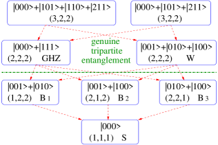
Figure 5: The partially ordered structure of multipartite pure entangled states in the $3\times 2\times 2$ format, including the $3$-qubit case. Each class, corresponding to the SLOCC orbit, is labeled by the representative, local ranks, and the name. Noninvertible local operations, indicated by dashed arrows, degrade ”higher” entangled classes into ”lower” entangled ones.

The onion structure consists of eight orbits on $M$ under SLOCC (see Fig. 4). Generic entangled states of the outermost class is given by nonzero ${\rm Det}A$, which can be calculated in the boundary format as the determinant associated with the Cayley-Koszul complex. Although this is one of the Gelfand et al.’s recent successes for generalized discriminants, we avoid its detailed explanation here. According to Theorem 3.3 of gelfand+94 , we have

$${\rm Det}A=m_{1}m_{4}-m_{2}m_{3}$$ (16)

of degree $6$, where $m_{j}\;(j=1,2,3,4)$ is the $3\times 3$ minor of

$$\left(\begin{array}[]{cccc}a_{000}&a_{001}&a_{010}&a_{011}\\ a_{100}&a_{101}&a_{110}&a_{111}\\ a_{200}&a_{201}&a_{210}&a_{211}\end{array}\right)$$ (17)

without the $j$-th column, respectively. Next, it is characteristic that $X^{\vee}_{\rm sing}$ is $X^{\vee}_{\rm node}(1)$ weyman+96 . Similarly to the $3$-qubit case in Sec. 4.1, $X^{\vee}_{\rm node}(1)$ means that the ”bipartite” matrix in Eq. (17) does not have the full rank, i.e., all four $3\times 3$ minors $m_{j}$ in Eq. (17) are zero. The SLOCC orbits which appear inside $X^{\vee}_{\rm sing}$ are essentially the same as the 3-qubit case.

Accordingly, we obtain the partially ordered structure of multipartite entangled states as Fig. 5. The tripartite entanglement consists of four classes. Because the class of $M\!-\!X^{\vee}$, whose representative is $|000\rangle\!+\!|101\rangle\!+\!|110\rangle\!+\!|211\rangle$, and that of $X^{\vee}\!-\!X^{\vee}_{\rm sing}$, whose representative is $|000\rangle\!+\!|101\rangle\!+\!|211\rangle$, have the same local ranks $(3,2,2)$, they do not convert each other in the same reason as GHZ and W do not. However, the former two classes of the local ranks $(3,2,2)$ can convert to the latter two classes of $(2,2,2)$ by noninvertible local operations (i.e., LOCC). And we can ”degrade” these tripartite entangled classes into the biseparable or completely separable classes by LOCC in a similar fashion to the $3$ qubits.

We notice that 3 grades in the $3$-qubit case changed to 4 grades in the $3\!\times\!2\!\times\!2$ ($1$-qutrit and $2$-qubit) case. In general, the partially ordered structure becomes ”higher”, as the system of each party becomes the higher dimensional one. We also see how the tensor rank note3 is inadequate for the onion-like classification of SLOCC orbits.

IV.3 $n\!\geq\!4$-qubit (format $2^{n}$) case

Further in the $n\!\geq\!4$-qubit case, our classification works. The outermost class $M(\!=\!{\mathbb{C}}P^{2^{n}\!-\!1})\!-\!X^{\vee}$ of generic $n$-partite entangled states is given by ${\rm Det}A_{n}\!\neq\!0$. In $n\!=\!4$, ${\rm Det}A_{4}$ of degree 24 is explicitly calculated by the Schläfli’s construction in Sec.3.2. It would be suggestive to transform any generic $4$-partite state (${\rm Det}A_{4}\!\neq\!0$) to the ”representative” of the outermost class by invertible local operations,

$$\alpha(|0000\rangle+|1111\rangle)+\beta(|0011\rangle+|1100\rangle)+\gamma(|0101\rangle+|1010\rangle)+\delta(|0110\rangle+|1001\rangle),$$ (18)

where the continuous complex coefficients $\alpha,\beta,\gamma,\delta$ should satisfy

$${\rm Det}A_{4}=\alpha^{2}\beta^{2}\gamma^{2}\delta^{2}(\alpha+\beta+\gamma+\delta)^{2}(\alpha+\beta+\gamma-\delta)^{2}(\alpha+\beta-\gamma+\delta)^{2}(\alpha-\beta+\gamma+\delta)^{2}\\ (-\alpha+\beta+\gamma+\delta)^{2}(\alpha+\beta-\gamma-\delta)^{2}(\alpha-\beta+\gamma-\delta)^{2}(\alpha-\beta-\gamma+\delta)^{2}\neq 0.$$ (19)

Thus three complex parameters remain in the outermost class (since we consider rays rather than normalized state vectors). This means that there are infinitely many same dimensional SLOCC orbits in the $4$ qubits, and the SLOCC orbits never locally convert to each other when their sets of the parameters are distinct. It is also the case for the $n\!>\!4$ qubits. Note that, in $n\!=\!4$, this outermost class $M\!-\!X^{\vee}$ corresponds to the family of generic states in Verstraete et al.’s classification of the $4$ qubits by a different approach (generalizing the singular value decomposition in matrix analysis to complex orthogonal equivalence classes), and $X^{\vee}$ contains their other special families verstraete+02 .

The next outermost class is $X^{\vee}\!-\!X^{\vee}_{\rm sing}$. In the $4$ qubits, $X^{\vee}_{\rm sing}$ is shown to consist of eight closed irreducible components of codimension 1 in $X^{\vee}$; $X^{\vee}_{\rm cusp},\>X^{\vee}_{\rm node}(\emptyset)$, and six $X^{\vee}_{\rm node}(j_{1},j_{2})$ for $1\!\leq\!j_{1}\!<\!j_{2}\!\leq\!4$ weyman+96 . They neither contain nor are contained by each other. Their intersections also give (finitely) many lower dimensional genuine $4$-partite entangled classes. Since the $4$-partite entangled classes necessarily have the same local ranks $(2,2,2,2)$, these classes are not interconvertible by noninvertible local operations (i.e., any LOCC). As typical examples, GHZ, the maximally entangled state in Bell’s inequalities gisin+98 ,

$$|{\rm GHZ}\rangle=|0000\rangle+|1111\rangle,$$ (20)

(i.e., $a_{0000}=a_{1111}\neq 0$ and the others are $0$) is included in the intersection of $X^{\vee}_{\rm node}(\emptyset)$ and six $X^{\vee}_{\rm node}(j_{1},j_{2})$, but is excluded from $X^{\vee}_{\rm cusp}$. In contrast, W,

$$|{\rm W}\rangle=|0001\rangle+|0010\rangle+|0100\rangle+|1000\rangle,$$ (21)

(i.e., $a_{0001}=a_{0010}=a_{0100}=a_{1000}\neq 0$ and the others are $0$) is included in the intersection of $X^{\vee}_{\rm cusp}$ and six $X^{\vee}_{\rm node}(j_{1},j_{2})$ but is excluded from $X^{\vee}_{\rm node}(\emptyset)$.

In the $n\!>\!4$ qubits, $X^{\vee}_{\rm sing}$ is shown to consist of just two closed irreducible components $X^{\vee}_{\rm cusp}$ and $X^{\vee}_{\rm node}(\emptyset)$ weyman+96 . We find that GHZ and W are contained not only in $X^{\vee}\>({\rm Det}A_{n}\!=\!0)$ but in $X^{\vee}_{\rm sing}$; i.e., they have nontrivial solutions in Eqs.(LABEL:eq:critical), satisfying the singular conditions. They correspond to different intersections of further singularities similarly to the $4$ qubits. In other words, they are peculiar, living in the border dimensions between entangled states and separable ones,

In brief, the dual variety $X^{\vee}$ and its singularities lead to the coarse onion-like classification of SLOCC orbits, when SLOCC gives infinitely many orbits. The partially ordered structure of multipartite pure entangled states becomes ”wider”, as the number $n$ of parties increases. Although many inequivalent $n$-partite entangled classes appear in the $n$ qubits, they never locally convert to each other, as observed in dur+00 . In particular, the majority of the $n$-partite entangled states never convert to GHZ (or W) by LOCC, and the opposite conversion is also not possible. This is a significant difference from the bipartite or $3$-qubit case, where almost any entangled states and the maximally entangled states (GHZ) can convert to each other by LOCC with nonvanishing probabilities.

V Conclusion

We have classified multipartite entanglement (SLOCC orbits) in a unified manner based on hyperdeterminants ${\rm Det}A$. The underlying idea is the duality between the set of completely separable states (the Segre variety $X$) and that of degenerate entangled states (its dual variety $X^{\vee}$ of ${\rm Det}A\!=\!0$). The generic entangled class of the maximal dimension is given by the outside of $X^{\vee}$, and other multipartite entangled classes appear in $X^{\vee}$ or its different singularities, seen in the onion picture like Fig. 3 or Fig. 4. Since the onion-like classification of SLOCC orbits is given by every closed subset, not only it is useful to see intuitively why, say in the $3$ qubits, the W class is rare compared to the GHZ class, but it can be also extended to the classification of multipartite mixed states (cf. the appendix of miyake02 ).

In virtue of this onion-like classification, we clarify the partially ordered structure, such as Fig. 5, of inequivalent multipartite entangled classes of pure states, which is significantly different from the totally ordered one in the bipartite case. Local ranks are not enough to distinguish these classes any more, and we need to calculate SLOCC invariants associated with ${\rm Det}A$. This partially ordered structure becomes ”higher” as the dimensions of subsystems enlarge, and it becomes ”wider” as the number of the parties increases.

This work reveals that the situation of the widely known bipartite or $3$-qubit cases, where the maximally entangled states in Bell’s inequalities belong to the generic class, is exceptional. Lying far inside the onion structure, the maximally entangled states (GHZ) are included in the lower dimensional peculiar class in general, e.g., for the $n\geq 4$ qubits. It suggests two points. The majority of multipartite entangled states can not convert to GHZ by LOCC, and vice versa. So, we have given an alternative explanation to this observation, first made in dur+00 by comparing the number of local parameters accessible in SLOCC with the dimension of the whole Hilbert space. Moreover, there seems no a priori reason why we choose GHZ states as the canonical $n$-partite entangled states, which, for example, constitute a minimal reversible entanglement generating set (MREGS) in asymptotically reversible LOCC bennett+00 ; wu+00 .

The onion-like classification seems to be reasonable in the sense that it coincides with the SLOCC classification when SLOCC gives finitely many orbits, such as the bipartite or $3$-qubit cases. So two states belonging to the same class can convert each other by invertible local operations with nonzero probabilities. On the other hand, when SLOCC gives infinitely many orbits, this classification is still SLOCC-invariant, but may contain in one class infinitely many same dimensional SLOCC orbits which can not locally convert to each other even probabilistically. For example, in the $4$-qubit case, the generic entangled class in Eq.(18) has three nonlocal continuous parameters. Note that it can be possible to make the onion-like classification finer, by characterizing the nonlocal continuous parameters in each class.

Then, we may ask, what is the physical interpretation of the onion-like classification in the case of infinitely many SLOCC orbits? Although a simple answer has yet to be found, we discuss two points. (i) Let us consider global unitary operations which create the multipartite entanglement. On the one hand, states in distinct classes would have the different complexity of the global operations, since they have the distinct number and pattern of nonlocal parameters. On the other hand, states in one class are supposed to have the equivalent complexity, since they just correspond to different ”angles” of the global unitary operations. (ii) We can consider the case where more than one states are shared, including the asymptotic case. Even in two shared states, there can exist a local conversion which is impossible if they are operated separately, such as the catalysis effect jonathan+99 . So we can expect that we do more locally in this situation and the coarse classification may have some physical significance. This problem remains unsettled even in the bipartite case.

Finally, three related topics are discussed. (i) The absolute value $|{\rm Det}A_{n}|$ of the hyperdeterminant, representing the amount of generic entanglement, is an entanglement monotone by Vidal vidal00 . This never conflicts with the property that the maximally entangled states in Bell’s inequalities (GHZ) generally has a zero ${\rm Det}A_{n}$. A single entanglement monotone is insufficient to judge the LOCC convertibility, and generic entangled states of the nonzero ${\rm Det}A_{n}$ can not convert to GHZ in spite of decreasing $|{\rm Det}A_{n}|$. (ii) The $3$-tangle $\tau=4|{\rm Det}A_{3}|$ first appeared in the context of so-called entanglement sharing coffman+00 ; i.e., in the $3$ qubits, there is a constraint (trade-off) between the amount of $2$-partite entanglement and that of $3$-partite entanglement. By using the entanglement measure (concurrence $C$) for the $2$-qubit mixed entangled states, this is written as $C^{2}_{1(23)}\geq C^{2}_{12}+C^{2}_{13}$, and $\tau$ is defined by $\tau=C^{2}_{1(23)}-C^{2}_{12}-C^{2}_{13}$ for the $3$-qubit pure entangled states. We expect that, in turn, the hyperdeterminant ${\rm Det}A_{n}$ gives a clue to find the entanglement measure of more than $2$-qubit mixed states. (iii) In the classification of mixed states, we can construct the so-called witness operator ${\mathcal{W}}$ in order to detect the entanglement of a given mixed state $\rho$ lewenstein+00 . It would be interesting to observe that since the optimal one ${\mathcal{W}}_{o}$ forms the tangent hyperplane ${\rm tr}(\rho{\mathcal{W}}_{o})=0$ to the set of separable mixed states, it shares the same ideas as our dual variety.

We hope that many intrinsic features of multipartite entanglement will be elucidated from hyperdeterminants.

Note added. For the 4-qubit case, a complete, generating set for polynomial invariants under SLOCC is calculated recently in luque+02 , which enables ${\rm Det}A_{4}$ expressed by the lower degree invariants.

References

- (1) e.g., C.H. Bennett and D.P. DiVincenzo (2000), Nature 404, 247; review articles (2001) in Quant. Info. Comp. 1.
- (2) N. Linden and S. Popescu (1998), Fortsch. Phys. 46, 567; A. Acín et al. (2000), Phys. Rev. Lett. 85, 1560; H.A. Carteret, A. Higuchi, and A. Sudbery (2000), J. Math. Phys. 41, 7932.
- (3) C.H. Bennett et al. (2000), Phys. Rev. A 63, 012307.
- (4) W. Dür, G. Vidal, and J.I. Cirac (2000), Phys. Rev. A 62, 062314.
- (5) SLOCC was tied to in dur+00 . Since we treat as a ray, i.e., an unnormalized vector, we rather relate SLOCC to .
- (6) The local rank can be defined as the rank of the reduced density matrix traced out for all except one party. Note that this definition is applicable to the multipartite case.
- (7) The enjoyable word ”onion” can be seen in A. Acín, D. Bruß, M. Lewenstein, and A. Sanpera (2001), Phys. Rev. Lett. 87, 040401, although their picture was drawn for mixed states.
- (8) H.K. Lo and S. Popescu (2001), Phys. Rev. A 63, 022301; and references therein.
- (9) A. Miyake (2002), quant-ph/0206111; to be published in Phys. Rev. A.
- (10) S. Hill and W.K. Wootters (1997), Phys. Rev. Lett. 78, 5022; W.K. Wootters (1998), ibid. 80, 2245.
- (11) V. Coffman, J. Kundu, and W.K. Wootters (2000), Phys. Rev. A 61, 052306.
- (12) As an excellent textbook of algebraic geometry, e.g., J. Harris (1992), Algebraic Geometry: A First Course (Graduate Texts in Mathematics 133, Springer-Verlag, New York). However, no preliminary knowledge of algebraic geometry is required in the text.
- (13) A. Miyake and M. Wadati (2001), Phys. Rev. A 64, 042317; and references therein.
- (14) For example, let us consider two Einstein-Podolsky-Rosen (EPR) pairs in the qubits. Since their local ranks are , we can not distinguish this state from genuine -partite entangled states (cf. Sec.4.3). In contrast, we readily find that the state is included in so that it is separable (not genuine -partite entangled).
- (15) A. Cayley (1845), Cambridge Math. J. 4 193; reprinted (1889) in his Collected Mathematical Papers (Cambridge Univ. Press, London/New York) 1, 80.
- (16) I.M. Gelfand, M.M. Kapranov, and A.V. Zelevinsky (1992), Adv. in Math. 96, 226.
- (17) I.M. Gelfand, M.M. Kapranov, and A.V. Zelevinsky (1994), Discriminants, Resultants, and Multidimensional Determinants (Birkhäuser, Boston), Chapter 14.
- (18) L. Schläfli (1852), Denkschr. der Kaiserl. Akad. der Wiss., math-naturwiss. Klasse, 4; reprinted (1953) in Gesammelte Abhandlungen (Birkhäuser-Verlag, Basel) 2, 9.
- (19) J. Weyman and A. Zelevinsky (1996), Ann. Inst. Fourier, Grenoble 46, 591.
- (20) If there exists a noninvertible local operation between SLOCC orbits, some of local ranks decrease. Note that the converse is generally not the case. However in our examples in Sec.4, we do find some noninvertible local operations for the decrease of local ranks.
- (21) The tensor rank means the number of terms in the minimal decomposition of in Eq.(1) by separable states. It coincides with the local rank in the bipartite case.
- (22) M. Koashi, V. Bužek, and N. Imoto (2000), Phys. Rev. A 62, 050302(R).
- (23) F. Verstraete, J. Dehaene, B. De Moor, and H. Verschelde (2002), Phys. Rev. A 65, 052112.
- (24) N. Gisin, and H. Bechmann-Pasquinucci (1998), Phys. Lett. A 246, 1; and references therein.
- (25) S. Wu and Y. Zhang (2000), Phys. Rev. A 63, 012308.
- (26) e.g., D. Jonathan, and M.B. Plenio (1999), Phys. Rev. Lett. 83, 3566.
- (27) G. Vidal (2000), J. Mod. Opt. 47, 355. The proof is given in the same way that the 3-tangle is proved an entanglement monotone in Appendix B of dur+00 , by generalizing the degree 4 of homogeneity of to of . It follows the arithmetic mean-geometric mean inequality that is greater than or equal to the average of resulted from any local POVM. The absolute value should be taken because is invariant up to sign under permutations of the parties.
- (28) M. Lewenstein, B. Kraus, J.I. Cirac, and P. Horodecki (2000), Phys. Rev. A 62, 052310; D. Bruß (2002), J. Math. Phys. 43, 4237.
- (29) J.-G. Luque and J.-Y. Thibon (2002), quant-ph/0212069.