Optical implementation of Deutsch-Jozsa and Bernstein-Vazirani
quantum algorithms in eight dimensions

Abstract

We report on a fiber-optics implementation of the Deutsch-Jozsa and Bernstein-Vazirani quantum algorithms for 8-point functions. The measured visibility of the 8-path interferometer is about 97.5%. Potential applications of our setup to quantum communication or cryptographic protocols using several qubits are discussed.

The last decade has seen the emergence of the field of quantum information processing. A particularly promising application is the concept of quantum algorithms, which allow certain problems such as factorizationShor or searchingGrover to be solved much faster than on a classical computer. Another algorithm which we will be interested in here is Deutsch’s algorithmDeutsch , the first quantum algorithm ever discovered, which was later generalized by Deutsch and JozsaDeutschJozsa (DJ). The DJ algorithm discriminates between a constant or a balanced $N$-point binary function using one single quantum query, while a classical algorithm requires ${\cal O}(N)$ classical queries. It was later on adapted by Bernstein and Vazirani (BV) for efficiently querying a quantum databaseBV ; BS .

In the present paper, we report on a fiber-optics implementation of the DJ algorithm using standard telecom optical components and a single-photon detector. The DJ algorithm has already been implemented using NMRnmr (see also nmr2 for a NMR implementation of the BV algorithm), table-top opticsDJoptical (optical demonstrations of other quantum algorithms also include Grover’s algorithmKwiat ; Amsterdam ), molecular statesmolecular , and very recently using an ion traptrap . However, our setup separates from these realizations (especially that of DJoptical ) on several major aspects. First, it relies on guided optics components, which makes it unnecessary to perform a precise alignment, and it is made robust against phase fluctuations by use of an autocompensation technique. Second, although it relies on linear optics, our realization is relatively efficient in terms of used optical resources compared to standard linear optical implementations of quantum computation. The central idea of such implementations consists in representing the basis states of a $N$-dimensional Hilbert space by $N$ optical paths so that unitary transformations are obtained by chaining linear optics components that make these paths interfereReck ; CerfKwiat . Such implementations seem, however, to be inherently inefficient since the space requirement (the number of optical components) and the time requirement both grow exponentially with the number $n$ of qubits (with $N=2^{n}$) fn . In contrast, in our setup, the number of components is kept linear in $n$, while the time needed still grows exponentially. Note that any implementation of an algorithm involving an arbitrary $2^{n}$-point function (also called oracle) does in any case require exponential resources to simulate this function. Therefore, the linear optical implementation of quantum algorithms involving oracles can reasonably be made as efficient as any other implementation in this respect. For all these reasons, our experimental demonstration works with a 8-point (3-qubit) function and might probably be extended even further without fundamental difficulty, while today’s largest size optical demonstrator of the DJ algorithm involves a 4-point functionDJoptical .

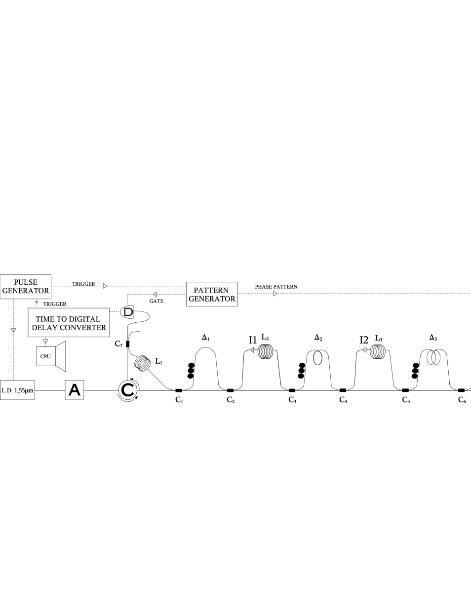
Figure 1: Fiber optics setup implementing the 8-dimensional Deutsch-Jozsa and Bernstein-Vazirani quantum algorithms.

Let us start by recalling the principle of the DJ algorithm. At the core of the algorithm is the oracle which computes a function $f(x)$, where $x\in\{0,1\}^{n}$ is an $n$ bit string, and $f\in\{0,1\}$ is a single bit. The DJ problem is to discriminate whether $f$ is a constant or balanced function, while querying the oracle as few times as possible. A balanced function is such that the number of $x$’s on which $f(x)=0$ is equal to the number of $x$’s on which $f(x)=1$. Classically, $2^{n-1}+1$ queries are necessary in the worst case, whereas the DJ algorithm requires a single query as we shall see. In this algorithm, $n$ qubits are used, and the basis of the Hilbert space is chosen as $|x\rangle=|x_{1}x_{2}\ldots x_{n}\rangle$ where $x_{i}\in\{0,1\}$. The quantum oracle carries out the transformation

$$|x\rangle|y\rangle\stackrel{{\scriptstyle\rm oracle}}{{\longrightarrow}}|x\rangle|y\oplus f(x)\rangle\ ,$$ (1)

where $|y\rangle$ is an ancilla qubit. By choosing $|y\rangle=(|0\rangle-|1\rangle)/\sqrt{2}$, the action of the oracle simplifies into

$$|x\rangle\stackrel{{\scriptstyle\rm oracle}}{{\longrightarrow}}(-1)^{f(x)}|x\rangle\ .$$ (2)

since $|y\rangle$ then remains unchanged.

The DJ algorithm starts with the system in the state $|0\rangle=|00\ldots 0\rangle$. Next, a Hadamard transform $H$ is applied independently on each of the $n$ qubit. Using the definition $H|x\rangle=2^{-n/2}\sum_{z\in\{0,1\}^{n}}(-1)^{x\cdot z}|z\rangle$, where $x\cdot z=\sum_{i}x_{i}z_{i}\bmod 2$ is the inner product of two $n$-bit strings, we see that the Hadamard transform acting on the initial state simply yields a uniform superposition of all states: $H|0\rangle=2^{-n/2}\sum_{x}|x\rangle$. This state is then sent through the oracle whereupon it becomes

$$2^{-n/2}\sum_{x}(-1)^{f(x)}|x\rangle\,.$$ (3)

The superposition principle allows the oracle to be queried on all input values in parallel. A second Hadamard transform is then carried out to obtain the state

$$2^{-n}\sum_{x,z}(-1)^{x\cdot z+f(x)}|z\rangle$$ (4)

which is finally measured in the $z$ basis. One easily deduces from Eq. (4) that when $f$ is constant, the probability of measuring $|0\rangle$ is one. In contrast, when $f$ is balanced, this probability is always zero, so the DJ algorithm can distinguish with certainty between these two classes of functions by querying the oracle a single time. The BV variant of this algorithm is also based on the transformation leading to Eq. (4). Suppose that the oracle is restricted to be of the form $f_{j}(x)=x\cdot j$ where $j\in\{0,1\}^{n}$ is an arbitrary $n$-bit string. The aim is to find the bit string $j$ with as few queries as possible. Classically one needs at least $n$ queries since each query provides one independent bit of information at most about $j$. Quantum mechanically, a single query suffices since using $f_{j}(x)$ in Eq. (4) shows that the measurement outcome is $z=j$ with probability.

Our all optical fiber (standard SMF-28) setup is illustrated in Fig. 1. Initially, a 3 ns light pulse is produced by a laser diode at $1,55~{}\mu$m, attenuated by an optical attenuator (Agilent 8156A), and then is processed through three unbalanced Mach-Zehnder (M-Z) interferometers with path length differences $\Delta_{l}$ ($l=1,2,3$) obeying $\Delta_{3}=2\Delta_{2}=4\Delta_{1}=15$ ns. Each MZ interferometer doubles the number of pulses so that, at the coupler C6, we get eight equally spaced pulses. This corresponds to the action of the Hadamard transform on the three input qubits in state $|0\rangle$. The pulses are then reflected by a Faraday mirror and, on their way back, are modulated by a phase modulator (Trilink) commanded by a pattern generator (Agilent 81110A) which selectively puts a phase shift of $0$ or $\pi$ on each pulse according to the 8-point function [see Eq. (3)]. The pulses then pass back through the three M-Z interferometers, thereby realizing a second triple Hadamard transform, and are sent via a circulator to a single-photon detector (id Quantique id200), which completes the DJ or BV algorithm. The additional delay lines $L_{1}$, $L_{2}$, and $L_{3}$, which obey $L_{3}>2L_{2}>4L_{1}>8\Delta_{3}$, ensure that the different outputs of the DJ or BV algorithm all reach the detector at different times. The delay lines $L_{2}$ and $L_{3}$ also contain an isolator so that the pulses are not transmitted on their way to the mirror. The photodetector was gated during 5 ns around the arrival time of each pulse by the pattern generator. The output of the detector was registered using a time to digital delay converter (ACAM-GP1) connected to a computer. All delays $\Delta_{i}$ and $L_{i}$ were chosen to be integer multiples of $\Delta_{1}$ within 0,2 ns. All electronic components were triggered by a pulse generator (Standford Research Inc. DG535). In order to maximize the visibility, polarization controllers were introduced in the long arm of each M-Z interferometer and in front of the polarization-sensitive phase modulator. Once optimized, the setup was stable for days.

This implementation of the DJ and BV algorithms differs from an earlier optical implementation of the DJ algorithmDJoptical in several important aspects. First, we run the algorithm for $n=3$ qubits and, more importantly, we measure all 8 outcomes, which makes it possible to realize the BV algorithm as well (the previous implementation DJoptical works with $n=2$ qubits and only measures the outcome $z=0$). Second, we operate at telecom wavelengths in optical fibers using a setup closely inspired from the “plug-and-play” quantum cryptographic system developed by Gisin and collaborators (see e.g. plugandplay ). For this reason, the present setup in a slightly modified version can be adapted to implement quantum cryptography using higher dimensional systemshighdQcrypto or to illustrate quantum communication complexity protocolsBCW over distances of a few kilometers. These potential applications will be discussed below. Third, the used resources are quite different in the two implementations: when scaled to a large $n$, the implementation of DJoptical requires exponential time and exponentially many optical elements, whereas our implementation also requires exponential time but only a linear number of optical elements. This is because the $n$ qubits are realized as $2^{n}$ separate optical paths in DJoptical , whereas in our case they are represented as $2^{n}$ light pulses traveling in a single optical fiber, extending naturally the “time-bin” realization of qubits used in plugandplay . The small number of optical elements in our setup therefore implies that it is relatively easy to increase the number of qubits $n$ while keeping the optical setup stable. As we shall see, a disadvantage of our setup is that the Hadamard transform can only be implemented with a probability of success of $1/2$. Since $2n$ Hadamard transforms are needed for the DJ algorithm with $n$ qubits, the resulting attenuation is $2^{-2n}$.

Let us now prove that our optical setup indeed realizes the DJ and BV algorithm. The quantum state describing the eight pulses at coupler C6 can be written as

$$|\psi\rangle\propto\sum_{x=000}^{111}\exp\left[i\sum_{l=1}^{3}(kx_{l}\Delta_{l}+\pi x_{l})\right]|\sum_{l=1}^{3}x_{l}\Delta_{l}\rangle$$ (5)

where $x$ stands for $(x_{1},x_{2},x_{3})$ and $|p\rangle$ denotes a pulse located at position $p$. The three bits $x_{1},x_{2},x_{3}=0,1$ label whether the pulse took the short ($x=0$) or the long ($x=1$) path through each interferometer. The factor $\exp[ik\sum_{l}x_{l}\Delta_{l}]$ with $k$ being the wave number takes into account the phase difference between a pulse traveling along the short or long paths of the interferometers. The factor $\exp[i\sum_{l}\pi x_{l}]$ takes into account the phase accumulated at the couplers: if the pulse takes the short path, it is transmitted at two couplers, whereas, if it takes the long path it is reflected twice. After reflection at the Faraday mirror and phase modulation, the pulses cross again the three M-Z interferometers and reach the photodetector in the state

$$|\psi\rangle\propto\sum_{x,y,z}(-1)^{f(x)}\exp\left[i\sum_{l=1}^{3}\left(k(x_{l}+y_{l})\Delta_{l}+\pi(x_{l}+y_{l}-y_{l}(z_{l}+z_{l+1})+{z_{l}+z_{l+1}\over 2})\right)\right]|\sum_{l=1}^{3}((x_{l}+y_{l})\Delta_{l}+z_{l}L_{l})\rangle$$ (6)

where the bits $y_{1},y_{2},y_{3}$ equal $0$ or $1$ according to whether the pulse passed through the short or the long path of each of the interferometers on its way back, and the bits $z_{1},z_{2},z_{3}$ equal $0$ or $1$ according to whether or not the pulse exited each of the interferometer in the path containing the delay lines $L_{1}$, $L_{2}$ or $L_{3}$. Note that we put $z_{4}=0$. We have again taken into account the phases induced by transmission or reflexion at the couplers C1-C6. The final state contains 120 pulses, but we are only interested in the eight pulses such that $x_{1}+y_{1}=x_{2}+y_{2}=x_{3}+y_{3}=1$, which are those that exhibit 8-path interference. The other pulses are filtered out in the computer analysis (they correspond to different time bins). The final state then becomes

$$|\psi\rangle\propto\sum_{z}(-i)^{z_{1}}(-1)^{z_{2}+z_{3}}\sum_{x}(-1)^{f(x_{1},x_{2},x_{3})+x_{1}(z_{1}+z_{2})+x_{2}(z_{2}+z_{3})+x_{3}z_{3}}|\Delta_{1}+\Delta_{2}+\Delta_{3}+z_{1}L_{1}+z_{2}L_{2}+z_{3}L_{3}\rangle$$ (7)

By relabeling the time bins according to the substitution $z_{1}\to z_{1}+z_{2}+z_{3}$ mod 2, $z_{2}\to z_{2}+z_{3}$ mod 2, and $z_{3}\to z_{3}$, this equation coincides (up to irrelevant phases and an overall normalization factor) with Eq. (4) with the 8 logical states $|z\rangle$ identified as specific time bins.

The setup thus realizes the DJ or BV algorithm, the main difference with an ideal algorithm being an extra attenuation by a factor of $2^{-7}$. A factor $2^{-3}$ originates from the couplers C2, C4, and C6 because each time a pulse passes through these couplers it only has a probability $1/2$ of exiting by the right path. Otherwise, it is absorbed by the isolators I1 and I2 or by the unconnected fiber pigtail at coupler C6. Another factor $2^{-3}$ is due to the filtering out of the 112 pulses produced on the way back that do not correspond to 8-path interferences. The remaining factor $2^{-1}$ is due to the coupler C7. This overall loss of 21 dB could be remedied by replacing the couplers C2, C4, C6, and C7 by optical switches which would direct the light pulses along the appropriate path. High speed, low loss optical switches are not available commercially at present, so we had to use couplers in the present experiment. However, we emphasize that this is a technological rather than a fundamental limitation.

In order to characterize the performances of our setup, we considered the $2^{n}$ oracles of the form $f_{j}(x)=x\cdot j$ and ${\overline{f}}_{j}(x)=x\cdot j+1{\rm~{}mod~{}}2$ (i.e., the oracles in the BV algorithm and their complements). For each oracle $f_{j}$ (or ${\overline{f}}_{j}$), we ran the algorithm 500,000 times and registered the number of counts in time bin $z$, denoted as $N_{j}(z)$ (or ${\overline{N}}_{j}(z)$). The algorithm gives constructive interference in the time bin $z=j$ for the oracle $f_{j}$ or ${\overline{f}}_{j}$, and destructive interference elsewhere. We then computed

$$V_{j}(z)={1\over 2}\left({N_{z}(z)-N_{j}(z)\over N_{z}(z)+N_{j}(z)}+{{\overline{N}}_{z}(z)-N_{j}(z)\over{\overline{N}}_{z}(z)+N_{j}(z)}\right)$$ (8)

for each pair of oracles with $j\neq z$, and calculated the visibility $V(z)$ in time bin $z$ by taking the average of $V_{j}(z)$ over all values of $j$. The measured visibilities $V(z)$ for 2 and 3 qubits are shown in Table I. Remarkably, they remain relatively high when going from 2 to 3 qubits in spite of the fact that 8 path interferences are involved. This is because the path differences are automatically compensated and only $n+1$ polarizations must be adjusted. It should therefore be relatively easy to go beyond $n=3$ without significantly decreasing the visibilities.

Because of the attenuation in our setup along with the quantum efficiency ($\simeq 10.5$ %) and the dark count probability ($\simeq 10^{-4}$ ns^-1) of our detector, the signal-to-noise ratio was not high enough to perform these visibility measurements in the single-photon regime. For this reason, in our experiment, approximatively 20 photons per pulse entered the phase modulator (oracle) in 4 dimensions, and approximatively 50 in 8 dimensions. However, minimal modifications should allow us to decrease the number of photons while keeping the signal-to-noise ratio constant. In particular, by reducing the pulse length or using two detectors instead of the coupler C7, it should be possible to operate in the single-photon regime in 4 (and possibly 8) dimensions. Moreover, as already mentioned, the Hadamard transform could be rendered deterministic by using fast low-loss optical switches instead of couplers, which would strongly reduce the losses.

z	1	2	3	4	5	6	7	8
$V(z)^{n=2}$	98.4	97.4	98.5	98.6
$V(z)^{n=3}$	96.78	97.99	97.68	97.32	97.33	97.56	97.37	97.28

Table 1: Measured average visibility $V(z)$ in the $z$th time bin for the DJ or BV algorithm with $n=2$ and $n=3$ qubits.

The present experiment can be extended in several ways. For example, one could implement the distributed Deutsch-Jozsa problemBCW where two parties, which receive each as input a $2^{n}$-bit string (denoted as $f$ and $g$), must decide whether $f=g$ or $f$ differs from $g$ in exactly $2^{n-1}$ bits (they are promised that only one of these two cases can occur). The value of $n$ for which the gap between the classical and quantum algorithms sets in is unknown, but recent results suggest that it could be as early as $n=4$ B . The distributed Deutsch-Jozsa algorithm could be realized with a slight modification of our setup in which the two parties, separated by by a few kilometers of optical fiber, would use each a phase modulator. This quantum protocol can also be easily adapted to multidimensional quantum cryptography, where two parties randomly choose their patterns $f$ and $g$. By publicly revealing part of $f$ and $g$, the parties can use the correlations between the measurement outcomes to establish a secret key. A detailed analysis shows that for n = 2, this exactly coincides with the 4-dimensional cryptosystem based on 2 mutually conjugate bases, which has been shown to present advantages over quantum cryptography in two dimensionsmultidimcrypto . A final potential application of this setup is to test quantum non locality using the entanglement-based Deutsch-Jozsa correlationsBCT . An entangled state of $2^{n}$ time bins must be produced, for example using the source RMZG , and each party must then carry out phase modulation and a Hadamard transform (which we have demonstrated are easy to realize on time bin entangled photons). The correlations between the chosen phases and the measured time of arrival of the photons at each side should exhibit quantum non locality. It has recently been shown that these correlations are non local for $n=4$ B , and that they exhibit exponentially strong resistance to detector inefficiency for large $n$ M , which means here that the 3 dB losses at each Hadamard transform can in principle be tolerated.

In summary, we have demonstrated, by implementing the DJ and BV algorithms for 3 qubits, a simple and robust method for manipulating multidimensional quantum information encoded in time bins in optical fibers. We anticipate that our method will have wide applicability for quantum information processing and quantum communication using higher dimensional systems.

It is a pleasure to thank N. Gisin, W. Tittel, G. Ribordy, H. Zbinden, and all the members of GAP optique for very helpful discussions and for providing the single-photon detector. We acknowledge financial support from the Communauté Française de Belgique under ARC 00/05-251, from the IUAP programme of the Belgian government under grant V-18, and from the EU under project EQUIP (IST-1999-11053).

References

- (1) P. W. Shor, SIAM J. Comput. 26, 1484 (1997)
- (2) L. K. Grover, Phys. Rev. Lett. 79, 325 (1997)
- (3) D. Deutsch, Proc. R. Soc. Lond. A 400, 97 (1985)
- (4) D. Deutsch and R. Jozsa, Proc. Roy. Soc. London Ser. A 439, 553 (1992)
- (5) E. Bernstein and U. Vazirani, SIAM J. Comput. 26, 1411 (1997)
- (6) B. M. Terhal and J. S. Smolin, Phys. Rev. A 58 (1998) 1822
- (7) J. A. Jones and M. Mosca, J. Chem. Phys. 109, 1648 (1998), N. Linden et al., Chem. Phys. Lett. 296, 61 (1998), R. Marx et al., Phys. Rev. A 62, 012310 (2000), K. Dorai et al., Phys. Rev. A 61, 042306 (2000)
- (8) J. Du et al, Phys. Rev. A 64, 042306 (2001)
- (9) S. Takeuchi, Phys. Rev. A 62 (2000) 032301
- (10) P. G. Kwiat et al., J. Mod. Opt. 47 (2000) 257-266
- (11) N. Bhattacharya et al., Phys. Rev. Lett. 88, 137901 (2002)
- (12) J. Vala et al., e-print quant-ph/0107058
- (13) R. Blatt, talk at the 3rd European QIPC Workshop, Dublin, 15-18 september 2002.
- (14) M. Reck et al, Phys. Rev. Lett. 73 (1994) 58.
- (15) N. J. Cerf, C. Adami, and P. G. Kwiat, Phys. Rev. A 57 (1998) R1477.
- (16) This exponential growth can be overcome in some cases (e.g. the optical implementation of Grover’s algorithm of Amsterdam , in which the number of optical elements remains constant although the space and time still grow exponentially).
- (17) G. Ribordy et al., Electronics Letters, 34 (22), 2116 (1998)
- (18) H. Bechmann-Pasquinucci and W. Tittel, Phys. Rev. A 61, 062308 (2000)
- (19) H. Buhrman, R. Cleve and A. Wigderson, Proceedings of the 30th Annual ACM Symposium on Theory of Computing, May 1998, pp. 63 - 68
- (20) V. Galliard, S. Wolf, and A. Tapp, e-print quant-ph/0211011
- (21) N. J. Cerf et al., Phys. Rev. Lett. 88, 127902 (2002)
- (22) G. Brassard, R. Cleve, A. Tapp, Phys. Rev. Lett. 83, 1874 (1999)
- (23) H. de Riedmatten et al., e-print quant-ph/0204165
- (24) S. Massar, Phys. Rev. A 65, 032121 (2002)