Geometric Phases and Topological Quantum Computation

Abstract

In the first part of this review we introduce the basics theory behind geometric phases and emphasize their importance in quantum theory. The subject is presented in a general way so as to illustrate its wide applicability, but we also introduce a number of examples that will help the reader understand the basic issues involved. In the second part we show how to perform a universal quantum computation using only geometric effects appearing in quantum phases. It is then finally discussed how this geometric way of performing quantum gates can lead to a stable, large scale, intrinsically fault-tolerant quantum computer.

1
Introduction

This review is on the nature of geometric phases in quantum mechanics and their use in quantum computation. I will introduce the notion of a geometric phase in a general way which is neither traditional nor historical. This will, I believe, help us appreciate the importance of this notion and also its generality - it is a phenomenon that has been discovered and exploited to explain a number of effects in many different areas of physics (see the collection of papers in [1]). One of the potential applications of this phase which is of interest to us is in quantum computation (the standard text is [2]). By using geometric phases to implement any elementary quantum gate we can therefore perform any quantum computation. The main reason why we would want to use geometrical phases for quantum computation is that frequently geometrical evolutions are easier to control and may also be more resistant to random noise coming from the environment. We will see, in Section $4$, how any quantum computation can be implemented by using purely geometric (topological) phases. This review is nether complete nor detailed - I have tried to emphasize points and connections that are usually neglected in literature, and to arrive at a potentially very important modern application in quantum computing. I have left a number of exercises and problems for the readers to address on their own. My intention is for the reader to acquire the basic flavor of the field which will then provide a good basis for a more independent study and work.

The review is organized as follows: In section $2$, I will review the notion of the geometric phase for the gauge invariant perspective. This section will also present a method of measuring geometric phases and discuss the classical analogue of the geometric phase. Various links with differential geometry will be emphasized. In section $3$, I review some basic notions in quantum computation and present some simple algorithms. This is a necessary background to be able to show why geometrical phases can be used to implement any quantum computation. Section $4$ then presents the most general way of implementing geometric quantum evolution, via the so called non-Abelian geometric phases. An example is given of a system that can support such an implementation. Section $5$, finally, summarizes the review and offers an outlook on the field.

2 Geometric Phases

Quantum states are represented as vectors in a complex vector space (with a few other properties we need not worry about here). However, these vectors are only defined up to a unit modulus complex number, or a phase in other words. So, the two states $|\xi\rangle$ and $e^{i\mu}|\xi\rangle$ are indistinguishable as far as quantum mechanics is concerned - no set of measurements can discriminate them. It is interesting that although this statement looks fairly innocent at first sight, it can lead to some very profound conclusions. The route we will take here and that turns out to be very fruitful is to think of this extra phase in a geometric way as well - where we represent the phase as a unit length vector in the complex plane diagram.

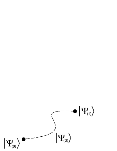
Figure 1: How do we compare phases of two different states when the probability between the states is the only experimentally well defined quantity in quantum mechanics?

Although we think of the amplitudes between two quantum states as fundamental entities in quantum theory, it is only the corresponding probabilities that we can ever observe experimentally. Therefore, given two states $|\psi_{i}\rangle$ and $|\psi_{f}\rangle$, we can only measure the mod square of their overlap, $|\langle\psi_{i}|\psi_{f}\rangle|^{2}$. What happens then if we wish to know the relative phase between these two states? Can we define their relative phase in spite of the fact that the absolute phase has no observable consequences? One idea to do so may be to look at the amplitude between the two states in the polar decomposition:

$$\langle\psi_{i}|\psi_{f}\rangle=re^{i\theta_{if}}$$ (1)

and define the phase $\theta_{if}$ as the relative phase between the two states. The main problem with this definition is that the states $e^{i\alpha}|\psi_{i}\rangle$ and $e^{i\beta}|\psi_{f}\rangle$ which differ from the original states by an overall arbitrary phase will have a different relative phases by the amount of $\Delta\theta=\alpha-\beta$. This is not very satisfactory as there are infinitely many choices for $\Delta\theta$ and they all look equally appropriate. We formally say that this definition of phase is gauge dependent (meaning “phase dependent”) - a feature that is considered negative as all observable quantities should be independent of the choice of the gauge. How about defining a path connecting the two states, $|\psi(s)\rangle$, such that when $s=0$ we have $|\psi_{i}\rangle$ and when $s=1$ we have $|\psi_{f}\rangle$ (see Fig 1)? Then we can transport the states $|\psi(s)\rangle$ from the position $i$ to the position $f$ and see how different the final phase is to that of $|\psi_{f}\rangle$ through interference. And if the states $|\psi_{f}\rangle$ and $|\psi_{i}\rangle$ transported to $|\psi_{f}\rangle$ interfere constructively, then they are in phase and if they interfere destructively, they are out of phase; the degree of interference can therefore define the phase difference (I will be as vague as possible about what kind of interference this is - I will be much more precise later on in subsection $2,5$). But which path do we choose and how do we know that the transport itself doesn’t introduce any additional “twists and turns” in the phases so that we are actually comparing some different phases to the original ones? This, in fact, is a well known problem in (differential) geometry (see [3] for an excellent introduction). Let’s state the problem in an abstract setting first (those of you familiar with general relativity will know immediately what I am taking about) and then specialize to quantum geometric phases.

2.1 Parallel Transport

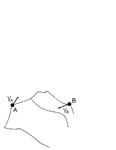
Figure 2: Comparing direction of two vectors at two different points is a non-trivial problem on a curved manifold. We have to somehow transport the vectors to the same point and then see what the angle between them is. Otherwise, comparing two vectors at different locations is difficult.

Suppose we have a curved manifold (as in Fig. 2) and we have a vector at a point $A$ and another at a point $B$. What is the angle between the two vectors (since phases in quantum mechanics can be thought of as vectors, this question is the same as our original question of relative phase between two quantum states). So, how do we measure the angle when the two vectors are at different positions? Well, we can transport one of them to the other one and then, when they are next to each other, the angle is easily measured (in the usual way as the “angular distance” between the vectors). But, again, we don’t want the transport itself to introduce any additional angles - we’d like it to be as “straight” as possible. The straightest possible path is known as a geodesic and the corresponding evolution along this path is known as the parallel transport (the usefulness of this concept in physics cannot be overemphasized - see [4]). To define a parallel transport, let’s look at the infinitesimal evolution, from $|\psi(s)\rangle$ to $|\psi(s+ds)\rangle$. If we don’t want there to be any twists and turns in the phase, even infinitesimally, then the two states should be in phase. So, we require that

$$\mbox{Arg}\{\langle\psi(s)|\psi(s+ds)\rangle\}=0$$ (2)

This is the same as asking that $\langle\psi(s)|\psi(s+ds)\rangle$ is purely real, i.e.

$$\mbox{Im}\{\langle\psi(s)|\psi(s+ds)\rangle\}=\mbox{Im}\{\langle\psi(s)|d|\psi(s)\rangle\}=0$$ (3)

up to second order. But $\langle\psi(s)|d|\psi(s)\rangle$ is purely imaginary anyway (prove it by differentiating $\langle\psi(s)|\psi(s)\rangle=1$ by $ds$), and hence the parallel transport condition becomes:

$$\langle\psi(s)|d|\psi(s)\rangle=0$$ (4)

If the evolution satisfies this equation, then the phase is said to be parallely transported, which is what we mentioned was required in order to be able to define a relative phase between two states (also see [5] for an accessible treatment of the phase parallel transport) . This definition of parallel transport is, however, not automatically gauge invariant. By this we mean that if instead of the state $|\psi(s)\rangle$, we use the state $|\tilde{\psi}(s)\rangle=e^{i\alpha(s)}|\psi(s)\rangle$, then the parallel transport condition changes by the amount

$$\langle\tilde{\psi}(s)|d|\tilde{\psi}(s)\rangle=\langle\psi(s)|d|\psi(s)\rangle+i\frac{d\alpha}{ds}ds$$ (5)

as can easily be checked. In order to obtain something that is gauge invariant we can integrate the expression $\langle\psi|d|\psi\rangle$ over a closed loop, giving us the expression for the geometric phase, and then exponentiate the result (the integral of $\frac{d\alpha}{ds}$ over a closed loop is $2\pi$, whose exponential is equal to unity). So, the geometric phase resulting from the parallel transport is

$$\gamma=\int_{i}^{f}\langle\psi(s)|\frac{d}{ds}|\psi(s)\rangle ds$$ (6)

and its exponential (over a closed loop) is gauge independent, but not path independent . Incidentally, note that we are requiring that the phase difference between every two infinitesimal points is zero. So, how come, if every infinitesimal difference is zero, that on a finite stretch a non-zero phase builds up? The answer is that the underlying space is curved and it is the curvature that is reflected in the phase difference; in fact, the curvature is equal the phase difference (up to a constant factor). When a quantity vanishes infinitesimally, but its integral over a finite region doesn’t, then this quantity is called non-integrable. Therefore, it can be succinctly said that geometric phases are a manifestation of non-integrable phase factors in quantum mechanics. Let’s look at a spin half system to illustrate this point.

2.2 The Bloch Sphere

Two level systems are ubiquitous in nature and can be used to store and manipulate any form of information (in quantum computing they are known as quantum bits or qubits). Two level systems are very conveniently represented on a sphere, such that all pure states lie on the surface of this sphere and all the mixed states are inside. There is a one-to-one correspondence between the points on and inside the sphere and quantum states of a two level system (Fig 3). This is because we need at most three parameters to specify every two level state, as can be seen from the general density matrix for the systems:

$$\rho=\frac{1}{4}(I+\sum_{i}s_{i}\sigma_{i})$$ (7)

where $\sigma_{i}$ are the Pauli spin matrices and $s_{i}=\mbox{tr}\sigma_{i}\rho$ are the $x,y,z$ coordinates on the sphere. If a state is pure than $s^{2}_{x}+s^{2}_{y}+s^{2}_{z}=1$ which, as we said, is a point on the surface of the sphere (a pure state in other words).

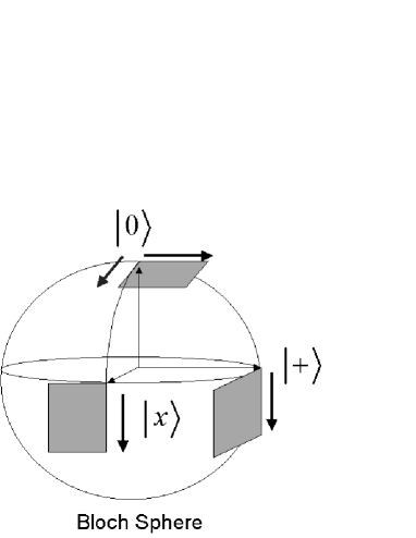
Figure 3: Parallel transport of the phase on the Bloch sphere. The presented evolution can be implemented in many different ways, one of which is the adiabatic Schrödinger equation as explained in the next section. The phase vector, initially at the North Pole and lying in the plane of the paper, for example, is then transported to the equator. After that, it moves on the equator, and makes a $90$ degrees shift, before coming back to the North Pole. The final phase vector, sticking out of the page, is at an angle to the initial vector which is also $90$ degrees.

Suppose that we now evolve from the state $|0\rangle$ to the state $|+\rangle=|0\rangle+|1\rangle$, then to $|x\rangle=|0\rangle+i|1\rangle$ and finally back to the state $|0\rangle$. On the Bloch sphere we are going from the North Pole to the Equator, then we move on the Equator by an angle of $\pi/2$ and finally we move back to the North Pole). What is the corresponding geometric phase? To see this we start with a tangential vector initially at the North Pole pointing in some direction (there are infinitely many directions corresponding to infinitely many arbitrary phases to start with). If we now parallely transport this vector along the described path, then we end up with a vector pointing in a different direction to the original one (even though, infinitesimally, the phase vector has always stayed parallel to itself!). The angle between the initial and the final vector is $\pi/2$, which is exactly equal to the area covered by the state vector during the transport, or the corresponding solid angle of the transport (the two are just different ways of phrasing the same thing and can be seen to be equivalent using Stokes’ theorem). Therefore, the two orthogonal states $|0\rangle$ and $|1\rangle$ evolve in the following way:

$$|0\rangle \rightarrow e^{i\Omega/2}|0\rangle$$ (8)

$$|1\rangle \rightarrow e^{-i\Omega/2}|1\rangle$$ (9)

where $\Omega$ is the solid angle (the factor of half is there because the orthogonal states are $\pi$ away from each other in the Bloch representation). This is important as it shows that orthogonal states pick up opposite phases of equal magnitude. The phase can be computed from the formula in eq. (6), but we note that it can also be written in a “discrete” way as

$$\arg\{\langle 0|+\rangle\langle+|x\rangle\langle x|0\rangle\}$$ (10)

This beautiful formula - originally due to Pancharatnam [1] - will be the basis of our general formulation of the geometric phase for pure states. From it we will be able to find that the space of quantum two level systems is curved. Are there, for that matter, any quantum states whose space is not curved (i.e. is flat) and how do we determine the curvature in general? If you want to measure a curvature at a point, then make a small loop around that point and compare the initial phase of your state to the phase after completing this loop. Suppose that the evolution is $|\psi(s_{i})\rangle\rightarrow|\psi(s_{i}+\delta s)\rangle\rightarrow|\psi(s_{i}+\delta s+\Delta s)\rangle\rightarrow|\psi(s_{i})\rangle$. Then, the final phase difference is (according to Pancharatnam)

$$\delta\theta = \arg\{\langle\psi(s_{i})|\psi(s_{i}+\delta s)\rangle\langle\psi(s_{i}+\delta s)|\psi(s_{i}+\delta s+\delta s^{\prime})\rangle\langle\psi(s_{i}+\delta s+\delta s^{\prime})|\psi(s_{i})\rangle\}$$ (11)

$$= \arg\{1+i(\frac{\delta}{\delta s}\langle\psi(s_{i})|\frac{\delta}{\delta s^{\prime}}|\psi(s_{i})\rangle-\frac{\delta}{\delta s^{\prime}}\langle\psi(s_{i})|\frac{\delta}{\delta s}|\psi(s_{i})\rangle)\}$$

$$= \frac{\delta}{\delta s}\langle\psi(s_{i})|\frac{\delta}{\delta s^{\prime}}|\psi(s_{i})\rangle-\frac{\delta}{\delta s^{\prime}}\langle\psi(s_{i})|\frac{\delta}{\delta s}|\psi(s_{i})\rangle$$ (12)

The definition of curvature, $K$, is $\delta\theta=K\delta A$, where $A$ is the area enclosed (this definition of curvature is due to Gauss). You can convince yourselves that for spin half particles $\delta\theta=\delta A$, which means that the curvature is $1$ (it is really $1/r^{2}$ as for any sphere, but the Bloch sphere has a unit radius). For optical coherent states, on the other hand, $\delta\theta=0$ (if we vary the phase and the amplitude of the state only), indicating that they line on a flat surface (which you can prove as an exercise, but see [6] for more details on the Riemannian structure of quantum states).

This formalism is very powerful and important in the modern formulation of physical theories (the so called gauge theories - see [4] for more details). But before we admire the beauty and cleverness of all this any further, let’s ask ourselves a very basic question: how do we actually (physically) implement the parallel transport given above?

2.3 Adiabatic implementation of parallel transport

Here we present one such implementation due to Berry [7], who actually discovered the quantum geometric phase in $1984$ in this way. A wavefunction of a system is a function of a set of parameters (which generally depend on time) and the time itself, $|\Psi(s(t),t)\rangle$. Suppose that the Hamiltonian is a function of $s$ only $H=H(s(t))$. Suppose, in addition, that these parameters change very slowly so that the system, which starts in a eigenstate of the initial Hamiltonian, stays an eigenstate of the instantaneous Hamiltonian, i.e.

$$H(s(t))|\Psi_{n}(s(t),t)\rangle=E_{n}(s(t))|\Psi_{n}(s(t),t)\rangle$$

(this is what is known as the adiabatic approximation in quantum physics- the other extreme is the sudden approximation where the Hamiltonian changes instantaneously). The Schrödinger equation for this system is

$$i\frac{d}{dt}|\Psi_{n}(s(t),t)\rangle=H(s(t))|\Psi_{n}(s(t),t)\rangle$$

(where we assume throughout that $\hbar=1$). We would like to show that the adiabatic evolution naturally implements the parallel transport of the phase of the quantum state. Note that apart from the adiabaticity assumption our analysis is completely general. Multiplying the Schrödinger equation by $\langle\Psi_{n}|$, and taking the eigenvalue equation into account we obtain:

$$i\langle\Psi_{n}|\frac{d}{dt}|\Psi_{n}\rangle=E_{n}$$

Now, every state gains a dynamical phase (as well as a geometric one) as it evolves. We’d like to get rid of the dynamical component of the phase and not take it into account when we are measuring the geometric contribution. To do so we define a new wavefunction by taking into account the dynamical phase

$$|\Phi_{n}(s(t),t)\rangle:=\exp\{iE_{n}(s(t))\}|\Psi_{n}(s(t),t)\rangle$$

which satisfies the following equation:

$$\langle\Phi(s(t),t)|\frac{d}{dt}|\Phi(s(t),t)\rangle=0$$

And this is the same as the parallel transport condition. So, the geometric part of the quantum phase is parallely transported when the state evolves under the Schrödinger equation in the adiabatic approximation. So can we derive a closed formula for the geometric phase? The answer is yes, and the solution to this equation is given by:

$$|\Phi(s(t),t)\rangle=e^{i\gamma(t)}|\Phi(s(t))\rangle$$

where

$$\frac{d}{dt}\gamma(t)=-i\langle\Phi(s(t))|\frac{d}{ds}|\Phi(s(t))\rangle\frac{ds}{dt}$$

We notice that the right hand side involves the 1-form $\beta$ describing the (symplectic) manifold of the projective Hilbert space - see Simon’s original differential geometric interpretation [8]. Therefore,

$$\frac{d}{ds}\gamma=\beta$$

where $\beta=-i\langle\Phi(s(t))|\frac{d}{ds}|\Phi(s(t))\rangle$. Integrating over a closed circuit $\partial S$ we solve for the Berry phase

$$\gamma=\oint_{\partial S}{\bf\beta}$$

Invoking Stokes’ theorem this becomes

$$\alpha=\int_{S}{\bf\sigma}$$

where $S$ is the area enclosed by the circuit $\partial S$ and ${\bf\sigma}$ is the 2-form on the symplectic manifold of the projective Hilbert space. This phase is called the Berry phase (the Berry and geometric phase are terms that I will use interchangeably, although this is by no means the standard convention in the literature).

In summary, the quantum phase arising in a general evolution of a quantum system consists of two parts: the dynamical part given by the formula

$$\delta=\int E(t)dt$$

and the geometric part, given by

$$\gamma=\int\langle\Psi(s)|\frac{d}{ds}|\Psi(s)\rangle\frac{ds}{dt}dt$$

The total phase is then the sum of the two contributions, $\phi=\delta+\gamma$.

We can encapsulate this whole subsection by saying that

The Schrödinger equation in the adiabatic limit implements the parallel transport of the phase of the evolving state.

In order to become more acquainted with the notion of geometric phases, we look at the classical analogue of this phenomenon.

2.4 Classical geometric phase

In this subsection we will talk about astronauts, cats and the Foucault pendulum in this section, all of which are classical objects. What do all these have in common? They all have the geometric phase at the root of their basic behaviour! Suppose an astronaut is in free space and initially facing away from his space ship. He wants to turn around by $180$ degrees to return to the ship, but there is nothing around him to push against or hold onto in order to turn around. His task may at first sight look impossible to achieve: his angular momentum is initially zero and in order to turn he seems to need to generate some angular momentum. But there are no forces externally, so this looks indeed impossible! However, anyone who has been observing cats knows that this reasoning is false. Cats face the same problem everyday and they manage to solve it. If a cat falls from a certain height and was initially upside down, she is still going to (almost always) land on her feet (hence the allegorical expression: “cats always land on their feet”). So, how do cats manage to apparently “violate the conservation of angular momentum”? Well, they don’t violate angular momentum conservation: they don’t use dynamics to turn, they use topology! Fig. 4 shows how the astronaut does something similar to the cat to turn around. Note that his hand movement is the same as the spin half evolution on the Bloch sphere - hence the angle by which he turns can be calculated in the same way.

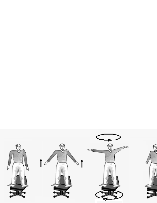
Figure 4: A person rotating while standing on the chair by using a purely geometrical effect while maintaining a zero angular momentum. In the position three, the person turns his arms around, and at the same time his body has to turn in the opposite direction to maintain zero angular momentum on the whole. Therefore by repeating the whole cycle a number of times, the person can make a rotation on the chair by any desired angle (try it for yourself!). This same effect is used by a cat to turn around in the air and land on the feel, even when initially being upside down.

Interestingly enough, the Foucault pendulum can be explained in the same geometric way [9]. Imagine that a pendulum is suspended at some latitude $\theta$, and that we observe its swinging motion as the Earth spins around its own axis. It is well known that the pendulum will after one rotation of the Earth swing in a plane at an angle to the original plane of motion. To see this, let us obtain an equation of motion of the pendulum. The Lagrangian for this problem is given by

$$L=\frac{1}{2}m(\frac{dx}{dt}^{2}+\frac{dy}{dt}^{2})-\frac{1}{2}m\omega^{2}(x^{2}+y^{2})-m\Omega\cos\theta(x\frac{dy}{dt}-y\frac{dx}{dt})$$ (13)

where $\Omega$ is the Earth’s frequency of rotation ($2\pi$ per day), $m$ is the mass of the pendulum and $\omega$ its natural frequency of swinging. The corresponding Euler-Lagrange equations of motion are easy to obtain (exercise!) and their solution written in the coordinate $z=x+iy$ is (in the adiabatic limit):

$$z(t)\approx x_{0}e^{-i\Omega\cos\theta t}e^{-i\omega t}$$ (14)

This form of the solution is convenient as it allows us to see two phases in the motion of the pendulum: the dynamical phase $\omega t$ which is the same as the quantum dynamical phase seen before and the geometric phase $\Omega\cos\theta t$. Note that after one day revolution of the earth, the geometric phase is $2\pi(1-\cos\theta)$ which is the same as the spin half geometrical phase. This is because our planet is a very good, albeit somewhat imperfect, physical representation of the Bloch sphere!

2.5 Experimental realization: The Pancharatnam connection

I now summarize the theory so far: we would like to compare phases of a quantum state at two different points. To do so we have to chose a path connecting the two points, and evolve one of the points along the path until it coincides with the other one. Then we interfere them to infer the phase. But how does this interference work?

Consider a conventional Mach-Zehnder interferometer in which the beam-pair spans a two dimensional Hilbert space $\tilde{{\cal H}}=\{|\tilde{0}\rangle,|\tilde{1}\rangle\}$ [10]. The state vectors $|\tilde{0}\rangle$ and $|\tilde{1}\rangle$ can be taken as (orthogonal) wave packets that move in two given directions defined by the geometry of the interferometer. In this basis, we may represent mirrors, beam-splitters and relative $U(1)$ phase shifts by the unitary operators

$$\tilde{U}_{M} = \left(\begin{array}[]{rr}0&1\\ 1&0\end{array}\right),\,\,\tilde{U}_{B}=\frac{1}{\sqrt{2}}\left(\begin{array}[]{rr}1&1\\ 1&-1\end{array}\right),$$ (19)

$$\tilde{U}(1) = \left(\begin{array}[]{cr}e^{i\chi}&0\\ 0&1\end{array}\right),$$ (22)

respectively. An input pure state $\tilde{\rho}_{in}=|\tilde{0}\rangle\langle\tilde{0}|$ of the interferometer transforms into the output state

$$\tilde{\rho}_{out} = \tilde{U}_{B}\tilde{U}_{M}\tilde{U}(1)\tilde{U}_{B}\tilde{\rho}_{in}\tilde{U}_{B}^{\dagger}\tilde{U}^{\dagger}(1)\tilde{U}_{M}^{\dagger}\tilde{U}_{B}^{\dagger}$$ (25)

$$= \frac{1}{2}\left(\begin{array}[]{cc}1+\cos\chi&i\sin\chi\\ -i\sin\chi&1-\cos\chi\end{array}\right)$$

that yields the intensity along $|\tilde{0}\rangle$ as $I\propto 1+\cos\chi$. Thus the relative $U(1)$ phase $\chi$ could be observed in the output signal of the interferometer.

Now assume that the particles carry additional internal degrees of freedom, e.g., spin (it is this degree of freedom that will be parallely transported). This internal spin space ${\cal H}_{i}\cong{\cal C}^{N}$ is spanned by the vectors $|k\rangle$, $k=1,2,\ldots N$. The density operator could be made to change inside the interferometer

$$\rho_{0}\longrightarrow U_{i}\rho_{0}U_{i}^{\dagger}$$ (26)

with $U_{i}$ a unitary transformation acting only on the internal degrees of freedom (we will see later on that this transformation need not be unitary, but could be a more general completely positive map). Mirrors and beam-splitters are assumed to leave the internal state unchanged so that we may replace $\tilde{U}_{M}$ and $\tilde{U}_{B}$ by ${\bf U}_{M}=\tilde{U}_{M}\otimes 1_{i}$ and ${\bf U}_{B}=\tilde{U}_{B}\otimes 1_{i}$, respectively, $1_{i}$ being the internal unit operator. Furthermore, we introduce the unitary transformation

$${\bf U}=\left(\begin{array}[]{rr}0&0\\ 0&1\end{array}\right)\otimes U_{i}+\left(\begin{array}[]{cr}e^{i\chi}&0\\ 0&0\end{array}\right)\otimes 1_{i}.$$ (27)

The operators ${\bf U}_{M}$, ${\bf U}_{B}$, and ${\bf U}$ act on the full Hilbert space $\tilde{{\cal H}}\otimes{\cal H}_{i}$. ${\bf U}$ corresponds to the application of $U_{i}$ along the $|\tilde{1}\rangle$ path and the $U(1)$ phase $\chi$ similarly along $|\tilde{0}\rangle$. We shall use ${\bf U}$ to generalize the notion of phase to unitarily evolving mixed states.

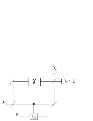
Figure 5: The Mach Zehnder interferometer intended to implement the measurement of the Pancharatnam phase. The internal degree of the system going through the interferometer is manipulated only in one branch of the interferometer. The manipulated branch is then interfered at the end with the non-manipulated branch to infer the phase difference.

Let an incoming state given by the density matrix $\varrho_{in}=\tilde{\rho}_{in}\otimes\rho_{0}=|\tilde{0}\rangle\langle\tilde{0}|\otimes\rho_{0}$ be split coherently by a beam-splitter and re-combine at a second beam-splitter after being reflected by two mirrors. Suppose that ${\bf U}$ is applied between the first beam-splitter and the mirror pair. The incoming state transforms into the output state

$$\varrho_{out}={\bf U}_{B}{\bf U}_{M}{\bf U}{\bf U}_{B}\varrho_{in}{\bf U}_{B}^{\dagger}{\bf U}^{\dagger}{\bf U}_{M}^{\dagger}{\bf U}_{B}^{\dagger}.$$ (28)

Inserting Eqs. (22) and (27) into Eq. (28) yields

$$\varrho_{out} = \frac{1}{4}\left[\left(\begin{array}[]{rr}\phantom{,}1&\phantom{-}1\\ 1&1\end{array}\right)\otimes U_{i}\rho_{0}U_{i}^{\dagger}+\left(\begin{array}[]{rr}1&-1\\ -1&1\end{array}\right)\otimes\rho_{0}\right.$$ (39)

$$+e^{i\chi}\left(\begin{array}[]{rr}1&1\\ -1&-1\end{array}\right)\otimes\rho_{0}U_{i}^{\dagger}$$

$$\left.+e^{-i\chi}\left(\begin{array}[]{rr}\phantom{,}1&-1\\ 1&-1\end{array}\right)\otimes U_{i}\rho_{0}\right].$$

The output intensity along $|\tilde{0}\rangle$ is

$$I \propto Tr\left(U_{i}\rho_{0}U_{i}^{\dagger}+\rho_{0}+e^{-i\chi}U_{i}\rho_{0}+e^{i\chi}\rho_{0}U_{i}^{\dagger}\right)$$ (40)

$$\propto 1+|Tr\left(U_{i}\rho_{0}\right)|\cos\left[\chi-\arg Tr\left(U_{i}\rho_{0}\right)\right],$$

where we have used $Tr(\rho_{0}U_{i}^{\dagger})=\left[Tr\left(U_{i}\rho_{0}\right)\right]^{\ast}$.

The important observation from Eq. (40) is that the interference oscillations produced by the variable $U(1)$ phase $\chi$ is shifted by $\phi=\arg Tr\left(U_{i}\rho_{0}\right)$ for any internal input state $\rho_{0}$, be it mixed or pure. This phase difference reduces for pure states $\rho_{0}=|\psi_{0}\rangle\langle\psi_{0}|$ to the Pancharatnam phase difference between $U_{i}|\psi_{0}\rangle$ and $|\psi_{0}\rangle$. Moreover the visibility of the interference pattern is $\nu=|Tr\left(U_{i}\rho_{0}\right)|\geq 0$, which reduces to the expected $\nu=|\langle\psi_{0}|U_{i}|\psi_{0}\rangle|$ for pure states.

It is clear from this experiment what it means to have a parallel transport of phase, i.e. no phase introduced during an infinitesimal evolution. We require that

$$\arg Tr\left(U(t,t+dt)\rho_{0}\right)=0$$ (41)

which is the same as the parallel transport condition presented before in eq. (4). Suppose for that matter that we have no dynamics and only projective transformations (the transformation $U$ is in this case no longer unitary, but the same above analysis still holds). Then $U=|\psi_{n}\rangle\langle\psi_{n-1}|...|\psi_{2}\rangle\langle\psi_{1}|$ so that the formula for the phase now becomes

$$\gamma=arg\{\langle\psi_{1}|\psi_{2}\rangle\langle\psi_{2}|\psi_{3}\rangle\ldots\langle\psi_{n}|\psi_{1}\rangle\}$$ (42)

which is known as the Pancharatnam phase. Now, this is the most general form of the phase for pure state, which leaves the motion between the states completely arbitrary: it could be adiabatic, and cyclic, but it could also be non-unitary and open. There are many advantages of expressing the phase in this way:

• it is aesthetically pleasing!

• it is manifestly gauge invariant since whenever we have the ket $|\psi_{j}\rangle$ in the expansion, we also have its bra present, $\langle\psi_{j}|$, meaning that all the extra phases of individual states cancel. Thus, states only appear as projectors which is the key to achieving independence of phase. As a slight digression, those of you who know a bit about the lattice gauge theory (see [11] for an excellent succinct introduction) will immediately notice the similarity with Wilson’s loop construction. In order to obtain the action leading to the geometric phase we have to sum up the infinitesimal loops, $W_{P}$, over all points $P$. Each loop is defined as

  $$W_{P}=\langle\psi(x_{P})|\psi(x_{P}+dx)\rangle...\langle\psi(x_{P}+dx+\delta x)|\psi(x_{P})\rangle$$ (43)

  After a simple manipulation and using the Baker-Hausdorff formula

  $$\exp(\lambda A)\exp(\lambda B)=\exp(\lambda(A+B)+\lambda^{2}/2[A,B]+O(\lambda^{3}),$$

  it can be shown that

  $$W_{P}=e^{iF_{\mu\nu}dx_{\mu}\delta x_{\nu}}$$ (44)

  where the fictitious geometric field strength is

  $$F_{\mu\nu}=\partial_{\mu}A_{\nu}-\partial_{\nu}A_{\mu}-i[A_{mu},A_{nu}]$$ (45)

  and the geometric potential (also called connection in the lectures) is

  $$A_{\nu}=\langle\psi(x)|\partial_{\nu}|\psi(x)\rangle$$ (46)

  To obtain the Wilson loop over a finite range we just need to add up all the infinitesimal loops such that $W=\sum_{P}W_{P}$. Pushing the analogy with gauge theories we can think of a fictitious topological charge $Q^{T}$ defined via Gauss’ law:

  $$\frac{1}{A}\oint B_{\mu\nu}dA=Q^{T}$$ (47)

  Also, a covariant derivative of a field $\Phi$ is given by

  $$\Phi_{;\alpha}=\partial_{\alpha}\Phi+iA_{\alpha}\Phi$$ (48)

  and the field satisfies the following well known identity

  $$F_{\mu\nu;\rho}+F_{\nu\rho;\mu}+F_{\nu\rho;\mu}=0$$ (49)

• the formulation is very general. Any most general quantum evolution (the so called Completely positive, trace preserving map) going through the states above will lead to the same phase. There are many issues in this generalization that are still unclear, but I will not make any comments on this as it would obscure the exposition (see Sjöqvist et al. [10] for details).

• offers us a way of generalizing the phase to mixed states (as averaging over the corresponding pure states).

So, the geometric phase is independent of dynamics and gauge-free, however, it does depend on the underlying geometry of the evolution. To what extent can we eliminate the sensitivity to geometry?

2.6 Topology: The Aharonov-Bohm effect

The Aharonov-Bohm effect [12] can be revisited and explained in terms of the geometrical phase notion. Whereas the curvature in the above examples was in some sense fictitious (i.e. not generated by a “real” field, but by the intrinsic curvature in the geometry of quantum states), the Aharanov-Bohm effect is a manifestation of the electro-magnetic field. From this perspective we can even say that

electro-magnetism is the gauge invariant manifestation of a non-integrable quantum phase factor.

In other words, this means that the electromegnetic field (more precisely the potential) can be derived by postulating that the Schrödinger equation is invariant under local phase change of the wavefunction.

The Aharonov-Bohm set-up is the best example that explores the effect of the electro-magnetic field on phase through a beam of electrons in a double connected region where the field strength is zero as in Fig. 6. The phase gained by the beam is

$$\exp\{\frac{-ie\Phi}{\hbar c}\}$$ (50)

where $\Phi$ is the flux of the field. This phase has been experimentally observed. We see that the phase is path dependent (which is another way of saying that it is non-integrable). Even though it is path dependent, if we make one round trip about the flux, then we always gain the same amount of phase no matter what the path is. This a nice topological feature of the Aharonov-Bohm phase; the phase is then dependent on the number of times the flux has been encircled (the so called winding number in topology). It is this topological feature that we would like to have when we implement quantum computation (this idea was first presented in a seminal paper by Kitaev [13]). However, we would like the topology to be of a non-abelian (i.e. non-commutative) character as we explain later on in the review.

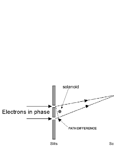
Figure 6: The Aharonov Bohm set up. A beam of electrons undergoes a double slit experiment with a solenoid placed behind the slits. The soleniod generates a magnetic field which is confined to the small region of the solenoid and is responsible for a shift in the interference pattern at a screen placed some large distance away.

3 Quantum Computation

So far we have explored connections between physics and geometry through the concept of the geometric phase which we saw is manifested both in quantum and classical mechanics. Now we plunge into another equally exciting and cross-disciplinary area: quantum information processing (see [2] for details).

All information is ultimately encoded in the most elementary quantum systems, so called quantum bits. A qubit is a quantum system in which the Boolean states $0$ and $1$ are represented by a prescribed pair of normalised and mutually orthogonal quantum states labeled as $\{|0\rangle,|1\rangle\}$. Unlike a simple Boolean variable, a qubit, typically a microscopic system such as an atom, a nuclear spin, or a polarised photon, can exist in an arbitrary superposition $\alpha|0\rangle+\beta|1\rangle$, making it more powerful as a computational resource.

In quantum computation, we set some register of qubits to an “input” state, evolve the qubits unitarily using simple building-block operations and then take the final state as “output”. More formally, a quantum logic gate is a device which performs a fixed unitary operation on selected qubits in a fixed period of time and a quantum network is a device consisting of quantum logic gates whose computational steps are synchronised in time. The outputs of some of the gates are connected by wires to the inputs of others. Also we define the size of the network to be the number of gates it contains.

3.1 Quantum logic gates and universality

The most common quantum gate is the Hadamard gate, a single qubit gate $H$ performing the unitary transformation known as the Hadamard transform. It is defined as

$$H=\frac{1}{\sqrt{2}}\left(\begin{array}[]{cc}1&1\\ 1&-1\end{array}\right)\mbox{\hskip 56.9055pt}\mbox{ \begin{picture}(30.0,0.0)(15.0,15.0)\put(-4.0,14.0){$|x\rangle$} \put(5.0,15.0){\line(1,0){5.0}} \put(20.0,15.0){\line(1,0){5.0}} \put(10.0,10.0){\framebox(10.0,10.0)[]{$H$}} \put(30.0,14.0){$\frac{(-1)^{x}\|x\rangle+|1-x\rangle}{\sqrt{2}}$} \end{picture} }$$ (51)

The matrix is written in the computational basis $\{|0\rangle,|1\rangle\}$ and the diagram on the right provides a schematic representation of the gate $H$ acting on a qubit in state $|x\rangle$, with $x=0,1$.

The addition of another single qubit gate, the phase shift gate $\mathbf{\phi}$, defined as $\left|\,0\right\rangle\mapsto\left|\,0\right\rangle$ and $\left|\,1\right\rangle\mapsto e^{i\phi}\left|\,1\right\rangle$, or, in matrix notation,

$${\mathbf{\phi}}=\left(\begin{array}[]{cc}1&0\\ 0&e^{i\phi}\end{array}\right)\mbox{\hskip 85.35826pt}\mbox{ \begin{picture}(30.0,0.0)(15.0,15.0)\put(-4.0,14.0){$|x\rangle$} \put(5.0,15.0){\line(1,0){20.0}} \put(20.0,15.0){\line(1,0){5.0}} \put(15.0,15.0){\circle*{3.0}} \put(14.0,19.0){$\phi$} \put(30.0,14.0){$e^{ix\phi}|x\rangle$} \end{picture} }$$ (52)

is actually sufficient to construct the following network (of size four), which generates the most general pure state of a single qubit (up to a global phase),

$$\mbox{ \begin{picture}(80.0,12.0)(0.0,3.0)\par\put(0.0,5.0){$|0\rangle$} \par\put(10.0,5.0){\line(1,0){10.0}} \put(20.0,0.0){\framebox(10.0,10.0)[]{H}} \put(30.0,5.0){\line(1,0){20.0}} \put(50.0,0.0){\framebox(10.0,10.0)[]{H}} \put(60.0,5.0){\line(1,0){20.0}} \par\put(40.0,5.0){\circle*{3.0}} \put(38.0,10.0){$2\theta$} \par\put(70.0,5.0){\circle*{3.0}} \put(65.0,10.0){$\frac{\pi}{2}+\phi$} \par\end{picture} }\quad\cos\theta|0\rangle+e^{i\phi}\sin\theta|1\rangle.$$ (53)

Consequently, the Hadamard and phase gates are sufficient to construct any unitary operation on a single qubit. We have used both the above gates in our discussion of the Pancharatnam phase in the Mach-Zehnder interferometer.

Thus the Hadamard gates and the phase gates can be used to transform the input state $|0\rangle|0\rangle...|0\rangle$ of $n$ qubits into any state of the type $|\Psi_{1}\rangle$ $|\Psi_{2}\rangle...$ $|\Psi_{n}\rangle,$ where $|\Psi_{i}\rangle$ is an arbitrary superposition of $|0\rangle$ and $|1\rangle.$ These are rather special $n$-qubit states, called the product states or the separable states. In general, a register of $n$ qubits can be prepared in states which are not separable, known as entangled states.

However, in order to entangle two (or more qubits) it is necessary to have access to two-qubit gates. One such gate is the controlled phase shift gate $B(\phi)$ defined as

$${B}(\phi)=\left.\left(\begin{array}[]{cccc}1&0&0&0\\ 0&1&0&0\\ 0&0&1&0\\ 0&0&0&e^{i\phi}\end{array}\right)\mbox{\hskip 42.67912pt}\mbox{ \begin{picture}(25.0,0.0)(0.0,20.0)\put(-4.0,14.0){$|y\rangle$} \put(-4.0,29.0){$|x\rangle$} \put(5.0,15.0){\line(1,0){20.0}} \put(5.0,30.0){\line(1,0){20.0}} \put(15.0,30.0){\circle*{3.0}} \put(15.0,15.0){\line(0,1){15.0}} \put(15.0,15.0){\circle*{3.0}} \end{picture}}\quad\right\}e^{ixy\phi}\left|\,x\right\rangle\left|\,y\right\rangle.$$ (54)

The matrix is written in the computational basis $\{|00\rangle,|01\rangle,|10\rangle,$ $|11\rangle\}$ and the diagram on the right shows the structure of the gate. Note: we know how to implement the single qubit phase gate geometrically, but not the other two gates aforementioned. Which gates are important to be able to implement in order to perform any quantum computation?

An important result in the theory of quantum computation states that the Hadamard gate, and all $B(\phi)$ controlled phase gates form an universal set of gates: if the Hadamard gate as well as all $B(\phi)$ gates are available then any $n$-qubit unitary operation can be simulated exactly with less than $C4^{n}n$ such gates, for some constant $C$ [2]. Consequently, being able to implement 1- and 2- qubit phase gates is of crucial importance in quantum computation. In the remaining part of the lectures we describe a new method for implementing the controlled phase gates based explicitly on geometric phases rather than dynamic ones. Thus if we show that the universal set can be implemented geometrically, then any computation can be implemented geometrically (see [14] for an NMR geometric implementation of the controlled phase gate).

3.2 Lightning review of quantum algorithms

Deutsch’s problem [15] is the simplest possible example which illustrates the advantages of quantum computation [16]. The problem is the following. Suppose that we are given a binary function of a binary variable $f:\{0,1\}\longrightarrow\{0,1\}$. Thus, $f(0)$ can either be $0$ or $1$, and $f(1)$ likewise can either be $0$ or $1$, giving altogether four possibilities. However, suppose that we are not interested in the particular values of the function at $0$ and $1$, but we need to know whether the function is: 1) constant, i.e. $f(0)=f(1)$, or 2) varying, i.e. $f(0)\neq f(1)$. Now Deutsch poses the following task: by computing $f$ only once determine whether it is constant or varying. This kind of problem is generally referred to as a promise algorithm, because one property out of a certain number of properties is initially promised to hold, and our task is to determine computationally which one holds.

First of all, classically finding out in one step whether a function is constant or varying is clearly impossible. We need to compute $f(0)$ and then compute $f(1)$ in order to compare them. There is no way out of this double evaluation. Quantum mechanically, however, there is a simple method to achieve this task by computing $f$ only once! We need to implement the following unitary transformation

$$|x\rangle\Rightarrow e^{i\pi f(x)}|x\rangle$$

where $x=0,1$. Now we can see where the power of quantum computers is fully realised: each of the components in the superposition of $|0\rangle+|1\rangle$ undergoes the same above evolution “simultaneously”, leading to the powerful “quantum parallelism”. This feature is true for quantum computation in general. Let us look at the two possibilities now:

1. if $f$ is constant, then the final state is

   $$|\Psi_{\mbox{out}}\rangle=\pm(|0\rangle+|1\rangle)\;.$$

   and

2. if, on the other hand, $f$ is varying, then, the final state is

   $$|\Psi_{\mbox{out}}\rangle=\pm(|0\rangle-|1\rangle)\;.$$

Note that the output qubit emerges in two different orthogonal states, depending on the type of $f$. These two states can be distinguished with $100$ percent efficiency. This is easy to see if we first perform a Hadamard transformation on this qubit, leading to the state $|0\rangle$ if the function is constant, and to the state $|1\rangle$ if the function is varying. Now a single projective measurement in $0,1$ basis determines the type of the function. Therefore, unlike their classical counterparts, quantum computers can solve Deutsch’s problem.

It should be emphasised that this quantum computation, although extremely simple, contains all the main features of successful quantum algorithms: it can be shown that all quantum computations are just more complicated variations of Deutsch’s problem. In particular, Shor’s algorithm for factorisation of numbers is just a scaled up version of Deutsch as it is based on period finding. Note, finally, that the main operation in Deutsch’s algorithm was the introduction of a phase conditional on the state of the qubit. This phase can, of course, be introduced in a purely geometrical way, by a spin-half encircling an area of the size of $2\pi$.

4 Topological implementation of quantum gates

Speaking somewhat loosely, we would now like to construct a universal set of quantum gates, which we know is impossible if we only have the (abelian) geometric phases (because we cannot implement a Hadamard transform with them). However, in addition to achieving the universality, we’d like to be able to achieve a certain degree of resistance to errors, but without performing any error correction. How far can this idea be pushed?

4.1 Non-abelian formalism

The best way of explaining the non-abelian phases is to look at how they arise during quantum evolution. The term “non-abelian” refers to the fact that two different phases don’t commute. Note that the ordinary (Berry) phases we discussed so far are abelian, i.e.

$$e^{i\gamma_{1}}e^{i\gamma_{2}}=e^{i\gamma_{2}}e^{i\gamma_{1}}$$

This inequality, however, would not be satisfied if we had non-abelian phases. This therefore implies that the non-abelian phases would not be represented by ordinary numbers, but by matrices. We now show that this scenario arises during the Schrödinger evolution in the adiabatic setting when our system is degenerate. Suppose that we have

$$H(t)|\psi_{1}(t)\rangle = E(t)|\psi_{1}(t)\rangle$$ (55)

$$H(t)|\psi_{1}(t)\rangle = E(t)|\psi_{1}(t)\rangle$$ (56)

and $\langle\psi_{1}(t)|\psi_{2}(t)\rangle=0$. From the Schrödinger equation we can conclude:

$$i\langle\psi_{1}|\frac{d}{dt}|\psi\rangle = E\langle\psi_{1}|\psi\rangle$$ (57)

$$i\langle\psi_{2}|\frac{d}{dt}|\psi\rangle = E\langle\psi_{2}|\psi\rangle$$ (58)

We recast this pair of equations by writing $|\psi\rangle=a_{1}(t)|\psi_{1}\rangle+a_{2}(t)|\psi_{2}\rangle$, and subtracting the dynamical phases by putting $E(t)=0$ (for all time $t$) we obtain

$$\frac{da_{1}}{dt}+a_{1}\langle\psi_{1}|\frac{d}{dt}|\psi_{1}\rangle+a_{2}\langle\psi_{1}|\frac{d}{dt}|\psi_{2}\rangle = 0$$ (59)

$$\frac{da_{2}}{dt}+a_{2}\langle\psi_{2}|\frac{d}{dt}|\psi_{2}\rangle+a_{1}\langle\psi_{2}|\frac{d}{dt}|\psi_{1}\rangle = 0$$ (60)

We can rewrite this equation as a vector-matrix equation,

$$\frac{dv}{dt}=i\left(\begin{array}[]{cc}i\langle\psi_{1}|\frac{d}{dt}|\psi_{1}\rangle&i\langle\psi_{1}|\frac{d}{dt}|\psi_{2}\rangle\\ i\langle\psi_{2}|\frac{d}{dt}|\psi_{1}\rangle&i\langle\psi_{2}|\frac{d}{dt}|\psi_{2}\rangle\end{array}\right)v$$

where

$$v(t)=\left(\begin{array}[]{c}a_{1}(t)\\ a_{2}(t)\end{array}\right)$$

The formal solution to this equation can be written in the usual “Dyson perturbative expansion”:

$$v(s)={\cal P}\exp\{i\int_{i}^{f}A^{j}(s)T_{j}ds\}v(0)$$

where ${\cal P}$ indicated the path-ordering operation of non-commuting factors $A^{j}(s)T_{j}$. This non-abelian phases is in general very difficult to evaluate, because of the path ordering operation. Note that if the state starts in the degenerate subspace it always remains there according to the adiabatic theorem .

I would like to mention potential advantages of using topological evolution to implement quantum gates. First of all, there is no dynamical phase in the evolution. This is because we are using degenerate states to encode information so that the dynamical phase is the same for both states (and it factors out as it were). Also, all the errors stemming from the dynamical phase are automatically eliminated. Secondly, the states being degenerate do not suffer from any bit flip errors between the states (like the spontaneous emission). So, the evolution is protected against these errors as well. Thirdly, the size of the error depends on the area covered and is therefore immune to random noise (at least in the first order) in the driving of the evolution. This is because the area is preserved under such a noise as formally proven by Palma [17]. Also, by tuning the parameters of the driving field it may be possible to make the phase independent of the area to a large extent and make it dependent only on a singular topological feature - such as in the Aharonov-Bohm effect where the flux can be confined to a small area - and this would then make the phase resistant under very general errors.

So, in order to see how this works in practice we take an atomic system as our model implementing the non-abelian evolution. We’ll see that quantum computation can easily be implemented in this way. The question, of course, is the one about the ultimate benefits of this implementation. Although there are some obvious benefits, as listed above, there are also some serious shortcomings, and so the jury is still out on this issue.

4.2 Example

Let’s look at the following $4$ level system analyzed by Unanyan, Shore and Bergmann [18]. They considered a four level system with three degenerate levels $1,3,4$ and one level $2$ with a different energy as in Fig 7. This system stores one bit of information in the levels $1$ and $2$ (hence there is double the redundancy in the encoding of information). We have the following Hamiltonian

$$H(t)=\left(\begin{array}[]{cccc}0&P(t)&0&0\\ P(t)&0&S(t)&Q(t)\\ 0&S(t)&0&0\\ 0&Q(t)&0&0\end{array}\right)$$

where $P,Q,S$ are some functions of time (to be chosen at leisure). It is not difficult to find eigenvalues and eigenvectors of this matrix (exercise!). There are two degenerate eigenvectors (with the corresponding zero eigenvalue for all times) which will be implementing our qubit and they are

$$\Phi_{1}(t)=\left(\begin{array}[]{c}\cos\theta(t)\\ 0\\ -\sin\theta(t)\\ 0\end{array}\right)$$

and

$$\Phi_{2}(t)=\left(\begin{array}[]{c}\sin\phi(t)\sin\theta(t)\\ 0\\ \sin\phi(t)\cos\theta(t)\\ -\cos\phi(t)\end{array}\right)$$

where $\tan\theta(t)=P(t)/Q(t)$ and $\tan\phi(t)=Q(t)/\sqrt{P(t)^{2}+Q(t)^{2}}$.

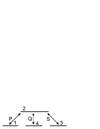
Figure 7: The four level system that can be used for non-abelian quantum computation to encode one qubit of information in two degenerate levels. The method is detailed in the text.

In the adiabatic limit (which we will assume here) these are the only important ones as the state will remain in their subspace throughout the evolution (this is guaranteed by the adiabatic theorem). Although, in general, the Dyson equation is difficult to solve, in this special example we can write down a closed form expression [18]. The unitary matrix representing the geometrical evolution of the degenerate states is

$$B(t)=\left(\begin{array}[]{cc}\cos\gamma(t)&\sin\gamma(t)\\ -\sin\gamma(t)&\cos\gamma(t)\end{array}\right)$$

where

$$\gamma(t)=\int\sin\phi(t)\frac{d\theta}{dt}dt$$ (61)

This therefore allows us to calculate the non-abelian phase for any closed path in the parametric space. After some time we suppose that the parameters return to their original value. So, at the end of the interaction we have the matrix

$$B(\infty)=\left(\begin{array}[]{cc}\cos\gamma_{f}&\sin\gamma_{f}\\ -\sin\gamma_{f}&\cos\gamma_{f}\end{array}\right)$$

where

$$\gamma_{f}=\oint_{c}\frac{Q}{(P^{2}+S^{2})\sqrt{Q^{2}+P^{2}+S^{2}}}(SdP-PdS)$$ (62)

which can be evaluated using Stokes’ theorem (the phase will in general depend on the path, as explained before). So, we can have a non-abelian phase implementing a Hadamard gate. With two systems of this type (mutually interacting) we can implement a controlled Not gate and therefore (at least in principle) have a universal quantum computer (see [19]). As an exercise I leave it to the reader to implement Deutsch’s algorithm in the purely topological way.

5 Conclusions and Outlook

We have seen what geometric phases are and appreciated their importance in physics in general. They were shown to be linked to the modern ideas of gauge theories and differential geometry, in particular the idea of parallel transport. In addition to their fundamental value, they also have a potential to implement quantum gates that are, at least in principle, more reliable than any existing gates. In order to do so I have argued that a high degree of topological dependence has to be achieved - i.e. independence of global geometry, which is certainly not that easy in practice. These topological gates will most likely have to be combined with other error correcting mechanisms in order to make a reliable quantum computer. The exact engineering design will, in the end, depend on the actual medium that is chosen to support quantum computation. It is fair to say that when this review was completed (in December 2002) there was no fully fault tolerant implementation of quantum computation. Fortunately there has been a huge number of proposals to implement such computations with various solid-state systems (such as Josephson Junctions and Quantum Dots), Nuclear Magnetic Resonance, Trapped Atoms and so on, and the whole field is, therefore, very much alive at present.

Acknowledgments. I have benefited greatly from discussions with J. Anandan, S. Bose, A. Carollo, A. Ekert, P. Falci, S. Fazio, I. Fuentes-Guridi, J. Jones, D. Markham, J. Pachos, M. Palma, M. Santos, J. Siewert and E. Sjöqvist on the subject of geometric phases. My research on this subject is supported by European Community, Engineering and Physical Research Council in UK, Hewlett-Packard and Elsag spa.

References

- [1] F. Wilczek and A. Shapre, Geometric phases in physics, (World Scientific, Singapore, 1990). All most important aspects of geometric phases, including its general formulation as well as numerous applications can be found in this book.
- [2] M. A. Nielsen and I. L. Chuang, Quantum Computation and Information, (Cambridge University Press, 2001). This is a very detailed exposition of quantum information and computation, covering both the theoretical basis as well as the more practical aspects. Excellent reference source.
- [3] C. W. Misner, K. S. Thorn and J. A. Wheeler, Gravitation, (W. H. Freeman, New York ).
- [4] T. Frankel, The Geometry of Physics, (Cambridge University Press, Cambridge, 2000).
- [5] J. Anandan, Nature 360, 307 (1992).
- [6] J.P Provost and G. Valle, Comm. Math. Phys. 76, 289 (1980).
- [7] M. V. Berry, Proc. Roy. Soc. A 329, 45 (1984).
- [8] B. Simon, Phys. Rev. Lett. 51, 2167 (1983).
- [9] R. T. Hammond, Contemp. Phys. 36, 103 (1995).
- [10] E. Sjöqvist et al, Phys. Rev. Lett. 85, 2845 (2000).
- [11] G. Münster and M. Waltrz, Lattice Gauge Theory: A Short Primer, lanl e-print archive, (2000).
- [12] Y. Aharonov and D. Bohm, Phys. Rev. 115, 485 (1959).
- [13] A. Yu. Kitaev, Fasult Tolerant Quantum Computation by Anyons, lanl e-print archive quant-ph (1997).
- [14] J. A. Jones, V. Vedral, A. Ekert and G. Castagnoli, Nature (2000); see also a proposal with Josephson Junctions in G. Falci, R. Fazio, G. M. Palma, J. Siewert, V. Vedral, Nature 407 355 (2000).
- [15] D. Deutsch and R. Jozsa, Proc. Roy. Soc. A 439, 553 (1992).
- [16] V. Vedral and M. B. Plenio, Prog. Q. Elect 22,1 (1998).
- [17] G. M. Palma, private communication.
- [18] R. G. Unanyan, B. W. Shore and K. Bergmann, Phys. Rev. A, 2910 (1999); see also L. M. Duan, J. I. Cirac and P. Zoller, Science 292, 1695 (2001).
- [19] P. Zanardi and M. Rasetti, Phys. Lett. A 264, 94 (1999).