Semiclassical Theory of Coherence and Decoherence

Abstract

A general semiclassical approach to quantum systems with system-bath interactions is developed. We study system decoherence in detail using a coherent state semiclassical wavepacket method which avoids singularity issues arising in the usual Green’s function approach. We discuss the general conditions under which it is approximately correct to discuss quantum decoherence in terms of a “dephasing” picture and we derive semiclassical expressions for the phase and phase distribution. Remarkably, an effective system wavefunction emerges whose norm measures the decoherence and is equivalent to a density matrix formulation.

I Introduction

The challenge of understanding to what extent a quantum system can retain its coherence in the presence of interactions with other degrees of freedom has attracted much attention. Much of it is motivated by recent advances in mesoscopicji ; sohn ; imry:book and cold-atom experimentsinguscio ; ketterle as well as keen interest in quantum computing, which depends crucially on quantum coherencedivincenzo ; nielson .

An essential ingredient in any discussion of coherence and decoherence is the identification of a “system” and a “bath” which interact with each other in such a way that a meaningful distinction can be made between the two. In the double slit experiment, for example, the electrons (or other quantum objects, e.g., “bucky balls”nairz ) are taken as the system and the degrees of freedom in the slits (phonons or spins, for example) are taken as the bath. Because the experiment only involves detecting the interference pattern on a screen behind the slits, no direct measurement of the bath (i.e. the slit degrees of freedom) is made. (Since one has no knowledge of the state of the bath one must sum over all possible states of the bath, i.e. one “traces over the bath”.) Only the system is directly observed. As is well knownfeyn2 , if the bath detects the path of the particle no interference pattern will be seen; the particle has therefore decohered. On the other hand, if there is no or only partial detection of the path of the particle by the bath, some interference pattern will be seen with its intensity reflecting the degree of coherence of the particlefeyn2 . We will later show how these familiar statements appear in a very transparent way in our semiclassical formalism.

The problem of a quantum system interacting with an environment has been addressed many times in the literature, e.g. feynman ; caldeira ; ady . The Feynman-Vernon influence functional approach is well known, although its usefulness beyond the context of harmonic baths has been an issue. The influence functional approach to more realistic systems has been advanced significantly by Makri and Thompsonmakri1 ; makri2 , exploiting and developing coherent state methods with smooth kernels suitable for Monte Carlo sampling. However, the generality of their approach necessarily means some detailed insights and limiting cases are lost in the machinery, so to speak.

Another approach is to make a semiclassical approximation for the system-bath evolution. Casting the system-bath interaction and the decoherence problem in terms of semiclassical wavepacket dynamics proves to be a useful and insightful exercise. Since a semiclassical approach is based on classical trajectories, one can present an intuitive picture of the criteria for coherence and decoherence in a coupled system-bath. One may imagine a more traditional van Vleck semiclassical Green’s function approach; however, this has the difficulty that caustic infinities abound in the van Vleck prefactors due ultimately to the failure of the stationary phase approximation in the limit of small action changes. For example, suppose we consider a harmonic oscillator and represent the $n^{th}$ state, $|n\rangle$, semiclassically so that $\langle x|n\rangle$ has singularities at the classical turning points for energy $E_{n}$. Suppose now we displace $|n\rangle$ slightly in position; call this $|\tilde{n}\rangle$. The semiclassical projections onto all of the original basis states $\langle n|\tilde{n}\rangle$ are completely wrong for small displacements. All but one of the projections are incorrectly predicted to be $0$ since their classical manifolds do not overlap, whereas the overlap with the undisplaced original state is nearly singular. The same displacement of the $n^{th}$ harmonic oscillator state, expanded in terms of localized Gaussians, is quite accurate; it has no such difficulties. Slight displacements of system or bath states is commonplace in the decoherence problem, so we avoid the caustic difficulties by starting with a wavepacket description, avoiding the singularities. We have called this the “oil on troubled waters” effect of using a wavepacket descriptionpostmodern .

One of the insights which emerges from this approach relates to recent discussions in the literature concerning the equivalence of a “bath overlap” picture of decoherence with a “system dephasing” picture. (See Stern, Aharonov and Imry (SAI)ady ; ady:nato ; imry:book and Feynman and Vernonfeynman .) We find that there are three main processes that contribute to decoherence: (i) Phase jitter (ii) Bath overlap decay and (iii) Shifts in the trajectory of the system wavepacket. We present explicit formulas for each of these effects within our semiclassical wavepacket description.

This paper is organized as follows. In Sec. II we develop the main ideas of our paper and derive the general expression for the coherence of a quantum system coupled to a general bath (described by a density matrix), Eq. (13). This expression can be recast in the form of a very intuitive effective system wavefunction, Eq. (14), which makes transparent the effects of system-bath interactions on the system (described by the norm of the effective wavefunction). In Sec. III we study several important cases of Eq. (13) and Eq. (14) in which certain physical process (phase jitter, etc.) dominate the system decoherence. In Sec. IV we summarize our main results and conclusions. Important supplementary material is presented in the appendixes. In Appendix A we detail how to compute the equations of motion perturbatively for Guassian wavepacket dynamics and derive expressions needed in the main text. In Appendix B we sketch the arguments of Stern, Aharonov and Imryady which equate “bath overlap” and “dephasing” in a special case system-bath interaction.

II Semiclassical Theory of Decoherence

We set out to construct a general formal context for decoherence, with the goal of reaching a useful and intuitive physical picture. The most general formal structure for decoherence (e.g. influence functionals for general anharmonic baths) would not involve semiclassical approximations, and could claim formal exactness. However such formulations must necessarily miss the mark on the issue of “useful and intuitive”.

It is helpful to have a specific model in mind. The model of a two armed device already introduced and used, for example, in the work of Stern, Ahronov and Imryady serves that purpose well. In Fig. 1, a wavepacket representing the system is coherently split into two pieces, one of which later interacts with a bath. The degree of coherence can be checked experimentally by combining the packets (as in the Aharonov-Bohm experiments of Ref.yacoby ), although it is more general to check ${\cal M}\equiv{\rm Tr}[\hat{\rho}_{\rm red}^{2}]$, where $\hat{\rho}_{\rm red}$ is the reduced density matrix for the system, after tracing over the bath variables.

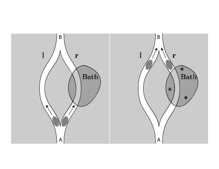
Figure 1: A wavepacket representing the “system” in a narrow waveguide is split coherently between two arms, one of which interacts with a “bath” of particles. Upon recombining on the other side, decoherence due to the system-bath interaction affects the interference (or lack of it) between the two arms.

An ambiguity in checking for interference fringes of the recombined beams is illustrated by supposing that there is a static potential maximum in the left arm but not the right, and no system-bath interaction in either arm. This will cause a time delay of the left wavepacket compared to the right, so no interference will result, even though the system is completely coherent. There are ways to avoid this, such as taking longer coherent wave trains initially for the system, but one must be careful, and other ambiguities can arise.

On the other hand, ${\cal M}$ is simply $1$ for a completely coherent system, and less than $1$ if some decoherence has taken place. For example, suppose we have a system wavepacket broken into two non-overlapping but coherent pieces, i.e. $\psi={1/\sqrt{2}}(\psi^{l}+\psi^{r})$, with $\langle\psi^{l}|\psi^{r}\rangle=0$ and $\langle\psi^{l}|\psi^{l}\rangle=\langle\psi^{r}|\psi^{r}\rangle=1$. Then the density matrix, $\hat{\rho}$, is

$$\hat{\rho}={1\over 2}\sum\limits_{i,j}|\psi^{i}\rangle\langle\psi^{j}|\;,$$ (1)

with $i$ and $j$ taking on the values $l$ and $r$. It is easily seen that ${\rm Tr}[\hat{\rho}]={\rm Tr}[\hat{\rho}^{2}]=1$, i.e. the system is completely coherent. However, if somehow the two parts $l$ and $r$ become completely decohered, (this in fact requires the action of more degrees of freedom–a bath) we loose the off diagonal elements of $\hat{\rho}$, getting

$$\bar{\hat{\rho}}={1\over 2}\left(|\psi^{l}\rangle\langle\psi^{l}|+|\psi^{r}\rangle\langle\psi^{r}|\right)\;.$$ (2)

Now we have ${\rm Tr}[\bar{\hat{\rho}}]=1$, but ${\rm Tr}[\bar{\hat{\rho}}^{2}]=1/2$.

This is not the end of decoherence for this system, if the left and right packets somehow undergo their own, “internal” decoherence. This “internal” decoherence will happen on a much longer time scale than the decoherence of the two initially coherent wavepackets because it is the difference in the interactions that each wavepacket experiences that determines the decoherence rate. This rate is almost always larger for two separated wavepackets than for a given wavepacket. All this is elementary, but it sets the stage for the more detailed work to follow.

Turning now to a discussion of our general problem of a system interacting with a bath, we cast our expressions in terms of density matrices. The most general density matrix for a bath expressed in terms of Guassian wavepackets is

$$\hat{\rho}_{\rm bath}=\sum_{i,j}w(i,j)|G_{i0}\rangle\langle G_{j0}|\;,$$ (3)

where $w(i,j)$ satisfies all the properties necessary so that $\hat{\rho}_{\rm bath}$ is a well-defined density matrix (${\rm Tr}_{\rm bath}\left[\hat{\rho}_{\rm bath}\right]=1,\left[w(i,j)\right]^{\dagger}=w^{*}(i,j)=w(j,i)$, etc.). In the special case of a pure state bath, we can write $w(i,j)=w_{i}w_{j}e^{i(\xi_{i}-\xi_{j})}$ where the $w_{i}$ are real, positive numbers and the $\xi_{i}$ are the associated phases. The states $|G_{i0}\rangle$ are multidimensional Gaussian wavepackets representing the bath states. Expanding the bath states in Gaussians allows us to make use of very intuitive notions of classical mechanics (which guide the wavepacket trajectories in the semiclassical approximation) while at the same time permitting us to overcome technical difficulties (singularities) in a more naive semiclassical treatment with van Vleck propagators.

Assuming that we take our system be the wavepacket initially split into two coherent pieces as shown in Fig. 1, the initial wavefunction of the system can be written as

$$|\psi_{\rm sys}\rangle={1\over\sqrt{2}}\left(|g_{0}^{l}\rangle+|g_{0}^{r}\rangle\right)\;,$$ (4)

where the states $|g_{0}^{r}\rangle$ and $|g_{0}^{l}\rangle$ are the right (r) and left (l) Gaussian wavepackets (coherent states) near the region A in Fig. 1. The density matrix for the system is then $\hat{\rho}_{\rm sys}=|\psi_{\rm sys}\rangle\langle\psi_{\rm sys}|$. Expressed in terms of Eq. (4),

$$\hat{\rho}_{\rm sys}={1\over 2}\left(|g_{0}^{l}\rangle+|g_{0}^{r}\rangle\right)\left(\langle g_{0}^{l}|+\langle g_{0}^{r}|\right)\;.$$ (5)

The total initial density matrix of the system and bath is then

$$\hat{\rho}_{\rm tot}(0)=\hat{\rho}_{\rm sys}\hat{\rho}_{\rm bath}\;.$$ (6)

To study the decoherence of the system due to interactions with the bath, we must compute the time evolution of Eq. (6). Our approach is to use the the perturbative wavepacket time evolution described in Appendix A. The key result is that the state

$$\left(|g_{0}^{l}\rangle+|g_{0}^{r}\rangle\right)|G_{i0}\rangle\stackrel{{\scriptstyle time}}{{\longrightarrow}}|g_{0t}^{l}\rangle|G^{l}_{it}\rangle+|g_{it}^{r}\rangle|G^{r}_{it}\rangle e^{i\phi_{i}}\;,$$ (7)

where $|g_{it}^{r,(l)}\rangle$ is the wavepacket of the system particle moving in the right (left) arm at time $t$ if the bath was in state $|G_{i0}\rangle$ initially. The state $|G^{r,(l)}_{it}\rangle$ is the perturbed wavepacket of the bath (according to Appendix A) at time $t$ for a particle moving in the right (left) arm where the bath was initially in state $|G_{i0}\rangle$. Note that since the particle in the left arm does not interact with the bath, $|G^{l}_{it}\rangle=|G^{0}_{it}\rangle$ and $|g_{it}^{l}\rangle=|g_{0t}^{l}\rangle$. The phase $\phi_{i}$ is given by Eq. (79).

We emphasize that it is the local nature of the Gaussian wavepackets combined with weak interactions that allows us to write down Eq. (7) with a product state for the piece of the wavefunction that interacted with the bath on the right arm. This approximation actually becomes exact as $\hbar\rightarrow 0$. It is precisely the lack of “local entanglement” (Eq. (7) still implies “global entanglement” of course) in the wavefunction that makes our approach conceptually convenient. In a more general basis, we would have a sum of terms for the right arm piece of the wavefunction and it would be difficult to identify physical phases of the type given by Eq. (79).

The total density matrix at later times thus becomes

$$\hat{\rho}_{\rm tot}(t)={1\over 2}\sum_{i,j}w(i,j) \left(|g_{0t}^{l}\rangle|G^{l}_{it}\rangle+|g_{it}^{r}\rangle|G^{r}_{it}\rangle e^{i\phi_{i}}\right)$$ (8)

$$\times\left(\langle g_{0t}^{l}|\langle G^{l}_{jt}|+\langle g_{jt}^{r}|\langle G^{r}_{jt}|e^{-i\phi_{j}}\right)\;,$$

which can be rewritten as

$$\hat{\rho}_{\rm tot}(t)=\hat{\rho}^{ll}(t)+\hat{\rho}^{lr}(t)+\hat{\rho}^{rl}(t)+\hat{\rho}^{rr}(t)\;,$$ (9)

where $\hat{\rho}^{ll}(t),\hat{\rho}^{lr}(t),$ etc. have the obvious meaning. To study the coherence of the system, we trace over the bath degrees of freedom to obtain the reduced density matrix,

$$\hat{\rho}_{\rm red} \equiv {\rm Tr}_{\rm bath}\left[\hat{\rho}_{\rm tot}\right]$$

$$= {\rm Tr}_{\rm bath}\left[\hat{\rho}^{rr}+\hat{\rho}^{rl}+\hat{\rho}^{lr}+\hat{\rho}^{ll}\right]\;,$$

which yields, for example,

$$\hat{\rho}_{\rm red}^{rl}={1\over 2}\sum\limits_{ij}|g_{it}^{r}\rangle\langle g_{0t}^{l}|w(i,j)e^{i\phi_{i}}{\cal O}_{ji}^{0r}\;,$$ (11)

where

$${\cal O}_{ji}^{0r}\equiv\langle G^{0}_{jt}|G_{it}^{r}\rangle\;,$$ (12)

with a similar expression for $\hat{\rho}_{\rm red}^{lr}$ (just the hermitian conjugate of $\hat{\rho}_{\rm red}^{rl}$) and the other terms. The bath wavepacket $|G_{jt}^{0}\rangle$ has a superscript $0$ to indicate that it is unperturbed from its trajectory if the system travels in the left arm. Note that $|g_{0t}^{l}\rangle$ does not interact with the bath and therefore does not develop an index $i$ depending on the bath state.

When $\hat{\rho}_{red}$ is squared and traced over to obtain the decoherence measure ${\cal M}\equiv{\rm Tr}\left[\hat{\rho}_{\rm red}^{2}\right]$, the terms ${\cal M}_{\rm coh}\equiv{\rm Tr}\left[\hat{\rho}_{\rm red}^{rl}\hat{\rho}_{\rm red}^{lr}+\hat{\rho}_{\rm red}^{lr}\hat{\rho}_{\rm red}^{rl}\right]$ contain all the information on inter-arm coherence. These give

$${\cal M}_{\rm coh} = {1\over 2}\sum\limits_{iji^{\prime}j^{\prime}}\langle g_{j^{\prime}t}^{r}|g_{jt}^{r}\rangle w(i^{\prime},j^{\prime})w(j,i){\cal O}_{j^{\prime}i^{\prime}n}^{r0}{\cal O}_{ij}^{0r}e^{i\phi_{j}-i\phi_{j^{\prime}}}$$ (13)

$$\equiv \langle\Psi^{\rm sys}|\Psi^{\rm sys}\rangle\;,$$

with

$$|\Psi^{\rm sys}\rangle={1\over\sqrt{2}}\sum\limits_{i,j}w(j,i){\cal O}_{ij}^{0r}e^{i\phi_{j}}|g_{jt}^{r}\rangle\;.$$ (14)

Remarkably, ${\cal M}_{\rm coh}$ is the self-overlap of a (generally non-normalized) effective system wavefunction. The emergence of a wavefunction form is unexpected because we have not specified that the bath was initially in a pure state; it may be in a mixed state such as a thermal bath. We can check Eq. (14) in the limit of no interaction with the bath: then, the overlap factors are all unity, the phases $\phi_{j}=0$, and all the gaussians $|g_{jt}^{r}\rangle$ are the same (normalized) unperturbed state $|g_{0t}^{r}\rangle$. Then,

$$|\Psi^{\rm sys}\rangle={1\over\sqrt{2}}\sum\limits_{i}w(i,i)|g_{0t}^{r}\rangle={1\over\sqrt{2}}|g_{0t}^{r}\rangle\;,$$ (15)

implying $\langle\Psi^{\rm sys}|\Psi^{\rm sys}\rangle={\cal M}_{\rm coh}=1/2$, i.e. maximum coherence.

Eqs. (13) and (14) are the central results of this section and they are the main formulas of this paper. They apply to any bath (harmonic or not, pure state or mixed state) with weak system-bath coupling and any number of total degrees of freedom.

Eq. (13) states that the system coherence is determined by an effective system wavefunction with wavepacket overlap factors $\langle g_{j^{\prime}t}^{r}|g_{jt}^{r}\rangle$, bath overlap factors ${\cal O}_{ij}^{0r}$, weighting factors (coming from the initial bath conditions) $w(j,i)$, and finally phase factors $e^{i\phi_{j}}$. The phases $\phi_{j}$ are classical actions divided by $\hbar$ and are given by Eq. (79). The “system wavefunction” overlap form, Eq. (14), is especially convenient for intuition and computation. Decoherence shows up as a reduction in the norm of the system wavefunction. This comes about from any or all of three factors: bath overlap decay, phase jitter, and system wavepacket displacement.

The are several more interesting facets of Eq. (13) deserving discussion. We will do this systematically, by considering important special cases which highlight aspects of this formula.

III Special Cases of Decoherence

We begin our discussion of various limits by assuming that the system overlaps and possibly also the bath overlaps are near unity. This regime is indeed accessible, since the classical action perturbation term is $\phi_{i}={1\over\hbar}\delta S_{t}$, where $\delta S_{t}$ is the action due to the perturbation along the unperturbed orbit. There is no doubt the action term can be large compared to $2\pi$ and vary widely, since the perturbing classical action can be large compared to $\hbar$. At the same time, the wavepacket displacement can remain small compared to its width, in both position and momentum space. Classical action changes are always accompanied by corresponding areas or volumes in phase space; if one plots the manifolds of the perturbed system exactly, then a phase $\phi=2\pi$ will be accompanied by a loop or area in phase space which is of this magnitude. However, the wavepacket width goes as $\sim\sqrt{\hbar}$, but the perturbing action increases as $\hbar^{-1}$. Therefore, for small enough perturbations and small enough $\hbar$, we can safely take the wavepacket overlaps to be 1, and focus on the phase terms.

Suppose that the system wavepackets $|g_{jt}^{r}\rangle$ are not displaced by the interaction with the bath, then we have

$$\langle g_{j^{\prime}t}^{r}|g_{jt}^{r}\rangle\approx 1$$ (16)

and Eq. (13) becomes

$${\cal M}_{\rm coh} = {1\over 2}\sum\limits_{iji^{\prime}j^{\prime}}w(i^{\prime},j^{\prime})w(j,i){\cal O}_{j^{\prime}i^{\prime}}^{r0}{\cal O}_{ij}^{0r}e^{i\phi_{j}-i\phi_{j^{\prime}}}$$ (17)

$$= {1\over 2}\left|\sum\limits_{i,j}w(j,i){\cal O}_{ij}^{0r}e^{i\phi_{j}}\right|^{2}\equiv{1\over 2}|\mu|^{2}\;.$$

If our bath had initially been in a pure state, $w(j,i)=w_{j}w_{i}^{*}$ so that

$$\mu = \sum_{ij}w^{*}_{i}{\cal O}_{ij}^{0r}e^{i\phi_{j}}w_{j}$$ (18)

$$= \int d\eta\,\chi_{l}^{*}(\eta)\chi_{r}(\eta)\;,$$

which is just a simple bath overlap. Here $\chi_{r(l)}$ is the state of the bath if the particle went around the right (left) arm; $\eta$ represents the set of bath coordinates. This is the notation of Appendix B.

In many physical situations, it may be the case that the largest contribution to the sum in Eq. (18) comes from $i=j$. (This might be the case because the bath overlaps ${\cal O}_{ij}^{0r}$ are small for $i\neq j$ and/or because the off-diagonal terms in $w^{*}_{i}w_{j}$ oscillate in sign from term to term.) Making this approximation, we find

$$\mu \approx \sum_{i}|w_{i}|^{2}e^{i\phi_{i}}{\cal O}_{ii}^{0r}\;.$$ (19)

This gives the interpretation of ${\cal M}_{\rm coh}$ as one half the modulus squared of a phase factor times a bath overlap averaged over different “runs”, or realizations of the bath, i.e.

$${\cal M}_{\rm coh}={1\over 2}|<e^{i\phi_{i}}{\cal O}_{ii}^{0r}>_{w_{i}}|^{2}\;.$$ (20)

From the system wavefunction viewpoint, we have (in the limit of Eq. (16)),

$$|\Psi^{\rm sys}\rangle=\left({1\over\sqrt{2}}\sum\limits_{i}|w_{i}|^{2}e^{i\phi_{i}}{\cal O}_{ii}^{0r}\right)|g_{0t}\rangle\;,$$ (21)

which lays the blame for decoherence entirely in the sum contained in the parentheses. This can be reduced in magnitude by both bath overlap decay factors or by phase jitter.

III.1 Nondynamical Bath

An important special case to consider is one in which the bath does not have any dynamics of its own, the so called “nondynamical” bath. The “nondynamical” bath limit emerges by further setting ${\cal O}_{ij}^{0r}=\delta_{ij}$ in Eq. (17) (or ${\cal O}_{ij}^{0r}=1$ in Eq. (19)), i.e. bath wavepackets undisplaced by the interaction, which would be the case indeed if the bath Hamiltonian commutes with the bath-particle interaction potential. Then,

$$|\Psi^{\rm sys}\rangle=\left({1\over\sqrt{2}}\sum\limits_{i}|w_{i}|^{2}e^{i\phi_{i}}\right)|g_{0t}\rangle\;.$$ (22)

The reduction of the norm (corresponding to decoherence) is due entirely to phase jitter. In this case we have a compelling formula emerging, in the spirit of SAI (See Appendix B),

$$\int d\eta\,\chi_{l}^{*}(\eta)\chi_{r}(\eta)=\sum\limits_{i}|w_{i}|^{2}e^{i\phi_{i}}\equiv<e^{i\phi_{i}}>\;,$$ (23)

where the phase $\phi_{i}$ is imparted with probability $|w_{i}|^{2}$: $\phi_{i}$ is the phase acquired if the bath wavepacket is $|G_{i0}\rangle$ initially, and this happens with probability $|w_{i}|^{2}$, the probability weight of that wavepacket in the initial bath. This formula gives a concrete picture of the nondynamical bath limit, and the origin of the phases which are averaged over: they are classical actions for the trajectory of the system-bath dynamics, divided by $\hbar$. In terms of ${\cal M}_{\rm coh}$, we have

$${\cal M}_{\rm coh}=\frac{1}{2}|<e^{i\phi_{i}}>|^{2}\;.$$ (24)

The limit of a nondynamical bath can also be achieved (without the bath Hamiltonian commuting with the bath-particle interaction potential) by a high temperature bath whose wavepacket description involves mostly very excited coherent states. Such coherent states are robust against self overlap decay, unless large energy exchange is occurring. This kind of nondynamical bath corresponds to classical states of the radiation field in a large cavity with high enough temperature. It is well known that this situation is described quantum mechanically in terms of excited coherent states of the field oscillators. Such baths (or similarly, externally applied fields) tend not to contribute to decoherence via a bath overlap decay mechanism for weak coupling, but rather the sort of “dephasing” expressed by Eq. (23).

III.2 Dynamical Bath

More generally, we see from Eq. (17) that the decoherence (still assuming little system displacement) arises from two sources: phase decoherence and amplitude decoherence (due to $|{\cal O}_{ii}^{0r}|<1$). The latter is caused by the bath wavepackets becoming displaced by interaction with the system. In this case, it is less compelling to associate $\langle e^{i\phi_{i}}\rangle$ with $\sum\limits_{i}|w_{i}|^{2}{\cal O}_{ii}^{0r}e^{i\phi_{i}}$, since the overlap factors are not naturally written as integrals over phase factors, although one could always do this, however absent of physical motivation. This situation corresponds to SAI’s dynamical bath. The present formulation shows a pure phase average picture for this case is somewhat forced. Bath wavepacket displacement (and in the next section, system wavepacket displacement) thus emerges as a restraint on a pure “dephasing” picture of decoherence.

The dynamical bath limit would be uninteresting if decoherence is always dominated by dephasing. But low temperature baths are prime suspects for overlap decay to dominate dephasing effects. For example, if there is just one bath coherent state, e.g. as in a $T=0$ bath whose true ground state is describe well by a single multidimensional coherent state, the Eq. (13) becomes

$${\cal M}_{\rm coh}\approx{1\over 2}|{\cal O}_{11}^{0r}|^{2}\;,$$ (25)

i.e. the decoherence is entirely caused by bath overlap decay. This is true even if the system wavepacket is strongly displaced, since the system wavepacket simply overlaps itself in Eq. (13) when there is but a single state in the sums. It is therefore possible to decohere from the zero temperature initial state or a given single coherent state of the bath, due to bath overlap decay; however, at zero temperature this requires degeneracies of the bath.

Here, it is especially clear that a phase average picture is not natural for a dynamical bath: in this case there is only one “quantum trajectory” so to speak, a single product wavepacket which describes the bath-system evolution in the right arm. Eq. (13) shows that the effect in this case is decoherence due to a displaced bath wavepacket.

III.3 System Overlap Decoherence

We now relax the artificial (though possible) condition that the system overlap terms are essentially $1$, i.e. the system wavepackets can be significantly displaced by interacting with the bath. The concepts of a dynamical and nondynamical bath still apply; the question at hand now is the further role of system overlap decay in forming the coherence measure ${\cal M}_{\rm coh}$. We assume a nondynamical bath to make the analysis simpler; this means that bath wavepacket self-overlaps are unity, and any decoherence can be blamed either on random phases (the dephasing limit) and/or on system overlap decay. We now investigate the relative importance of these two.

The relevant effective system wavefunction is then

$$|\Psi^{\rm sys}\rangle={1\over\sqrt{2}}\sum\limits_{i}|w_{i}|^{2}e^{i\phi_{i}}|g_{it}^{r}\rangle\;.$$ (26)

The self overlap of this wavefunction is

$${\cal M}_{\rm coh}={1\over 2}\sum\limits_{ij}|w_{i}|^{2}|w_{j}|^{2}\ e^{i\phi_{i}-i\phi_{j}}\langle g_{jt}^{r}|g_{it}^{r}\rangle\;.$$ (27)

The phase and overlap contributions are manifest. It is not possible to give a general rendition of the relative importance of phase and overlap contributions to this expression; this will depend on the system and bath under consideration. However, the diagonal terms always survive, even in the limit of strong kicking of the system wavepackets. (We remind the reader that even though our analysis was perturbative for the wavepacket displacements, in the sense of classical perturbation theory, the displacements can be strong in the quantum sense. “Strong” is measured by wavepacket overlap decay, which can be severe even while classical perturbations are correctly giving the wavepacket displacements. See Appendix A.) Restoring the bath overlap factors for a moment, for the diagonal terms we get

$${\cal M}_{\rm coh}\approx{1\over 2}\sum\limits_{i}|w_{i}|^{4}|{\cal O}_{ii}^{0r}|^{2}\leq{1\over 2}\sum\limits_{i}|w_{i}|^{4}\;.$$ (28)

Since $\sum\limits_{i}|w_{i}|^{2}=1$,

$$\sum\limits_{i}|w_{i}|^{4}\sim 1/N\;,$$ (29)

is an inverse participation ratio, where $N$ is the number of participating quantum states describing the bath. When $N$ is large, Eq. (29) predicts that ${\cal M}_{\rm coh}$ will be vastly smaller than $1/2$, effectively meaning the system is completely decohered in this limit. This is the limiting form in the strong system-kicking limit and makes physical sense: the broader the distribution of quantum states in the initial bath (measured by $N$ in Eq. (29), the more uncertain the “potential” felt by the system (bath has a broad distribution of possible states) and hence the greater the decoherence.

There remains a question, however: could the system overlap decay strongly as above without strong phase randomization, so that a pure dephasing picture would miss it? When one considers, for example, the harmonic model, the conclusion is soon reached that for finite temperature it is not easy to strongly displace the system wavepackets randomly without strong phase randomization.

IV Conclusions

In this paper, we have presented a semiclassical, wavepacket-based formalism for decoherence. We have limited ourselves to the case of a single system wavepacket split initially into two mutually coherent pieces, one of which interacts with a bath. We derive an expression for the measure of coherence in the system, Eq. (13), which determines the coherence in terms of wavepacket overlap factors $\langle g_{j^{\prime}t}^{r}|g_{jt}^{r}\rangle$, bath overlap factors ${\cal O}_{ij}^{0r}$, weighting factors (coming from the initial bath conditions) $w(j,i)$, and finally phase factors $e^{i\phi_{j}}$. The phases $\phi_{j}$ are classical actions divided by $\hbar$ and are given by Eq. (79).

One perhaps surprising and potentially very computationally and intuitively useful aspect of our formulation is the emergence of an effective system wavefunction, which measures the decoherence, Eq. (14): Decoherence shows up as a reduction in the norm of the system wavefunction. Similar ideas have been introduced in the context of a stochastic Schrodinger equation strunz .

After the derivation of the general formulas for the coherence of a quantum system interacting with a bath in Sec. II, we discuss several special limits of the interaction. In one limit, discussed in Sec. III.1, neither system nor bath wavepackets are significantly displaced by the interaction, but a distribution of phases develop which decohere the system. This is limit is naturally described as “dephasing” and is appropriate to a number of physical situations where the system-bath interactions are quite weak. In Sec. III.2 a situation is discussed where system wavepackets are barely perturbed but bath wavepackets are significantly displaced. In this limit, one can still force a random phase picture, but the identification with an average over random phase factors is more of a mathematical equivalence than a physically motivated idea. Finally, if the system wavepacket is strongly perturbed by the interaction, as in Sec. III.3, a new decoherence mechanism sets in: system overlap decay. Such system disturbance is hardly rare or unlikely. Strong perturbation of the system can occur with or without significant bath displacement.

Our perturbation treatment has certain similarities to linear response theory. For chaotic systems (expected for say a liquid or gaseous bath) it could suffer the same criticism vanK that the actual magnitude of the perturbation for which the formalism is valid is unreasonably small. However, it might benefit from the same saving graces as linear response theory; namely, that ensembles of trajectories are better behaved than individual trajectories.

The distinction we are making between phase randomization versus overlap decay has long been central within the context of spectroscopy of systems embedded in a bath (see, e.g. Ref. skinner ). The concepts of “dephasing”, “depopulation”, and “pure dephasing” are traditional in spectroscopy. Within the context of exponential decay, the relation

$${1\over T_{2}}={1\over 2T_{1}}+{1\over T_{2}^{*}}$$ (30)

is legion, where $T_{2}$ is the dephasing time, $T_{1}$ is the depopulation time, and $T_{2}^{*}$ is the pure dephasing time. The translation of concepts into the present discussion is: “dephasing” $\to$ “decoherence”; “pure dephasing” $\to$ “dephasing”. The time $T_{2}$ is typically the time constant for decay of the initial wavefunction created by absorption of a photon, and is measured from the width of of an absorption line. (If we had introduced a tunnel coupling between the two arms of our model device, we could also have had a natural population decay-the probability of being in each arm. This is an interesting subject for future study).

The approach we have taken to decoherence is not limited to the physical circumstances used here. The semiclassical wavepacket-perturbation approach should be applicable to wide variety of situations and physical measurables including electron decoherence in metalschakr ; altshuler ; zaikin ; cohen and studies of the classical-quantum correspondencebertet . We hope to pursue some of these in the near future.

Appendix A Coherent States and Gaussian Wavepackets

We present a brief review of Gaussian wavepacket dynamics for our approach to the decoherence problem. It is well known that the problem of the usual kinetic energy operator with a time dependent potential at most quadratic in the coordinates is exactly solvable, and is especially simple in the case of initial wavefunctions which are Gaussian; these remain exactly Gaussian wavepackets under the time evolution.

We note that our goals extend far beyond such quadratic systems; we will see that a semiclassical approximation permits the use of quadratic form dynamics in more general contexts. We make use of the so-called “thawed guassian approximation”thefirst ; thesecond ; thethird which employs the auxiliary variables ${\bf Z}$ and ${\bf P_{Z}},$ whose dynamics are given by the equations below. The “thawed Gaussian approximation” allows one to approximate the potential locally as quadratic thus taking advantage of the exactness of Gaussian propagation on quadratic potentials.

In a multidimensional form, a general Gaussian wavepacket is given by

$$\psi({\bf q},t)=\exp\{{i\over\hbar}[( {\bf q}-{\bf q_{t}})^{T}\cdot{\bf A_{t}}\cdot({\bf q}-{\bf q_{t}})$$ (31)

$$+{\bf p_{t}}\cdot({\bf q}-{\bf q_{t}})+s_{t}]\}\;,$$

where ${\bf A}_{t}$ is an $N\times N$ matrix for $N$ coordinates describing the stability of the center of the Gaussian wavepacket, and ${\bf q_{t}},\,{\bf p_{t}}$ are $N$-dimensional vectors describing the position and momentum evolution of the center of the wavepacket. We have introduced the more conventional wavepacket notation ${\bf q_{t}}={\bf q}(t)$, etc. Let the classical Hamiltonian, ${\rm H=T+V}$, have the usual Cartesian kinetic energy operator and a general time dependent potential ${\rm V}$ smooth at least up to quadratic order in the coordinates. The parameters of the Gaussian then obeytdwp ; leshouches

$${d\over dt}\bf q_{t} = \,\nabla_{p}{\rm H}$$ (32)

$${d\over dt}\bf p_{t} = \,-\nabla_{q}{\rm H}$$ (33)

$${\bf A_{t}} = {1\over 2}{{\bf P_{Z}}\cdot{\bf Z^{-1}}}$$ (34)

$${d\over dt}\left(\begin{array}[]{c}{\bf P_{Z}}\\ {\bf Z}\end{array}\right) = \,\left(\begin{array}[]{cc}{\bf 0}&{-{\bf V^{\prime\prime}}{(t)}}\\ {\bf m^{-1}}&{\bf 0}\end{array}\right)\left(\begin{array}[]{c}{\bf P_{Z}}\\ {\bf Z}\end{array}\right)$$ (41)

$$\dot{s}_{t} = \,{L_{t}}+{i\hbar\over 2}{\rm Tr[\dot{\bf Z}\cdot{\bf Z^{-1}}]}\;,$$ (42)

where $L_{t}$ is the usual classical Lagrangian. Integrating over time, we have

$$s_{t} = \,s_{0}+S_{t}+{i\hbar\over 2}{\rm Tr[\ln{\bf Z}]}\;,$$ (43)

where ${\bf V^{\prime\prime}}$ and ${\bf m^{-1}}$ are N-dimensional matrices of mixed second derivatives of the Hamiltonian with respect to position and momentum coordinates, respectively. That is,

$$\left[{\bf V^{\prime\prime}}\right]_{ij}={\partial^{2}{H}\over\partial q_{i}\partial q_{j}}\;,$$ (44)

and so forth. $S_{t}$ is the usual classical action. Eqs. (32-42) holds for a general time dependent ${\rm V}$. We focus on the stability equations, Eq. (41), which admit the solution

$$\left(\begin{array}[]{c}{\bf P_{Z_{t}}}\\ {\bf Z_{t}}\end{array}\right)={\bf M}(t)\left(\begin{array}[]{c}{\bf P_{Z_{0}}}\\ {\bf Z_{0}}\end{array}\right)\;,$$ (49)

where

$${\bf M}(t)={\hat{T}}\ e^{\int^{t}{\bf K}(t^{\prime})\ dt^{\prime}}\;,$$ (50)

and ${\hat{T}}$ denotes the time ordering operator, needed because

$${\bf K}(t)=\left(\begin{array}[]{cc}{\bf 0}&{-{\bf V^{\prime\prime}}(t)}\\ {\bf m^{-1}}&{\bf 0}\end{array}\right)$$ (53)

does not commute with itself (in general) at different times. ${\bf M}(t)$ is the usual classical stability matrix, where ${\bf M}_{11}=\partial p_{t}/\partial p_{0}$, etc.

Consider a narrow (in q) Gaussian wavepacket centered on the classical position ${\bf q_{0}}$ and momentum ${\bf p_{0}}$. Assuming a reasonably smooth potential, let us expand around ${\bf q_{0}}$ up to quadratic terms, arguing that the tails of the Gaussian are negligible where the Taylor expansion starts to break down. We use this quadratic form to propagate the packet in the next time instant. Thus the Gaussian will propagate in the next instant according to Eqs. (32-42). If we agree to move the center of the Taylor expansion to the moving mean position of the wavepacket, ${\bf q_{t}}$, then Eqs. (32-42) will hold, since the potential is now, by construction, a time dependent quadratic form. However, the interpretation has changed–the position and momentum parameters ${\bf q_{t}}$ and ${\bf p_{t}}$ are now just exactly the usual classical trajectories on the exact, anharmonic potential, but the distortion of the wavepacket is governed by the local quadratic expansion of the potential–thus keeping the wavepacket Gaussianthefirst . We illustrate the idea in Fig. 2.

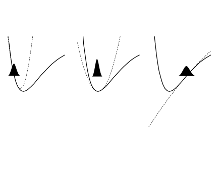
Figure 2: A Gaussian wavepacket in an anharmonic potential is approximately propagated by expanding the potential to quadratic order locally around the instantaneous center of the Gaussian.

In general this approximation breaks down after some time due to wavepacket spreading, but that time can be put off as long as we please as $\hbar\to 0$, since we can take a narrower wavepacket, with position and momentum uncertainties going as $\sqrt{\hbar}$. This delays the spreading by at least a factor $\sim 1/|\log\hbar|$ in time (for chaotic systems)logtime ; logtime2 ; logtime3 ; logtime4 .

Since any quantum state (aside from spin states) can be built out of Gaussians, we have a full semiclassical approach, exact as $\hbar\to 0$. Each Gaussian is propagated with its own optimized time-dependent Hamiltonian.

The phase $s_{t}$ of Eq. (43) is the usual action, taken along the guiding trajectory, modified by an extra term which takes the place of a Maslov phase. This term evolves smoothly in time and therefore is another advantage of a wavepacket approach as compared to the more troublesome eigenfunctions of Hermitian operators.

There are other approaches based on wavepackets which share the smoothing property, such as a full semiclassical coherent state propagatorweissman1 ; weissman2 ; cohst:little . This differs from the above Gaussian wavepacket (GWP) method in that the propagator is optimized for both the initial Gaussian and a final Gaussian onto which it is projected. It is also the “natural” semiclassical approximation if one retains stationary phase as the defining idea while passing to a coherent state basis. The coherent state method is usually more accurate at the same value of $\hbar$ compared to GWP, but it suffers several complexities. Foremost among these is that complex classical trajectories come in, (albeit for real time) with their attendant analytical difficulties including Stokes lines. Therefore, we choose the GWP approach as a best compromise between accuracy and complexity. In the semiclassical limit, $\hbar\to 0$, there is no accuracy compromise.

Perturbation theory may seem limited in scope at first glance, but we soon realize that strong interaction with many bath degrees of freedom leads to such rapid and near complete decoherence that an analysis of the strong system-bath coupling regime seems a little post mortem. We therefore focus our attention on the weak coupling limit.

In the setup in Fig. (1), we have a Hamiltonian given by

$$\hat{H}=\hat{H}_{\rm p}+\hat{H}_{\rm b}+\hat{V}\equiv\hat{H}_{0}+\lambda\hat{V}_{1}\;,$$ (54)

where $\hat{H}_{\rm p}$ ($\hat{H}_{\rm b}$) is the Hamiltonian of the particle (bath) and $\hat{V}$ is the coupling between them. Suppose we have solved the $\hat{H}_{0}=\hat{H}_{\rm p}+\hat{H}_{\rm b}$ problem, and now we wish to include the effects of $\lambda\hat{V}_{1}$, the system-bath interaction. In accordance with perturbation theory, the first order effect is determined by the extra potential felt by the wavepacket as it travels over its old trajectory. Assuming this perturbation is smooth as a function of coordinates, we include only terms linear in the interaction strength, $\lambda$. We can include perturbations to quadratic order as well, at the cost of increased complexity, but we defer this for future work. A weak interaction with a bath will show up in two ways in the wavepacket given in Eq. (31): (1) Changes to the guiding trajectory, $q_{t}$ and $p_{t}$ and (2) changes to the phase $s_{t}$.

A.0.1 Perturbation of the Guiding Trajectory

Let ${\bf q_{0}}(t)$ be the solution of the $\hat{H}_{0}$ problem for a particular trajectory. The first order perturbed solution we take to be ${\bf q}(t)={\bf q_{0}}(t)+\lambda\delta{\bf q}(t)$, ${\bf p}(t)={\bf p_{0}}(t)+\lambda\delta{\bf p}(t)$. By substituting this into Hamilton’s equations, we find that $\delta{\bf q_{t}},\delta{\bf p_{t}}$ obey

$${d\over dt}\left(\begin{array}[]{c}{\bf\delta p_{t}}\\ {\bf\delta q_{t}}\end{array}\right) = \,\left(\begin{array}[]{cc}{\bf 0}&{-{\bf V^{\prime\prime}}(t)}\\ {\bf m^{-1}}&{\bf 0}\end{array}\right)\left(\begin{array}[]{c}{\bf\delta p_{t}}\\ {\bf\delta q_{t}}\end{array}\right)+\left(\begin{array}[]{c}{\bf f}(t)\\ {\bf 0}\end{array}\right)\;,$$ (63)

where $f(t)=-V_{1}^{\prime}({\bf q_{0}}(t))$ is the time dependent forcing function. The solution is

$$\left(\begin{array}[]{c}{\bf\delta p_{t}}\\ {\bf\delta q_{t}}\end{array}\right) = {\bf\large M}(t)\left(\begin{array}[]{c}{\bf\delta p_{0}}\\ {\bf\delta q_{0}}\end{array}\right)+{\bf\large M}(t)\int\limits_{0}^{t}{\bf M}(t^{\prime})^{-1}\left(\begin{array}[]{c}{\bf f}(t^{\prime})\\ {\bf 0}\end{array}\right)dt^{\prime}$$ (71)

$$= {\bf\large M}(t)\int\limits_{0}^{t}{\bf M}(t^{\prime})^{-1}\left(\begin{array}[]{c}{\bf f}(t^{\prime})\\ {\bf 0}\end{array}\right)\ dt^{\prime},$$ (75)

since $\bf\delta p_{0}=\delta q_{0}=0$ in the present circumstances, with

$${\bf M}(t)^{-1}={\hat{T}}^{\dagger}\ e^{-\int^{t}{\bf K}(t^{\prime})\ dt^{\prime}}\;,$$ (76)

and ${\hat{T}}^{\dagger}$ forces the reverse order of times; i.e. earliest times to the left in the series expansion of ${\bf M}(t)^{-1}$. Note that $(d/dt){\bf M}(t)^{-1}={\bf M}(t)^{-1}{\bf K}(t)$. Thus, the perturbation of a general trajectory in classical mechanics generates a linearly forced oscillator problem. This is not surprising, since the small additional potential creates small new forces on the particle near its old trajectory.

A.0.2 Perturbation of the Phase

To see how the phase of the wavepacket changes under the perturbation, we examine

$$\delta s_{t} = \delta S_{t}$$ (77)

$$= \delta\int(T-V_{0}-\lambda V_{1})\ dt^{\prime}$$

$$= \delta\int(T-V_{0})\ dt^{\prime}-\delta\int\lambda V_{1}\ dt^{\prime}\;.$$

We see the change comes in two parts. The first is the change in the “old” action (it involves the old $V_{0}$) due to the new trajectory. Assuming the new one has not wandered too far, we have

$$\delta\int(T-V_{0})dt^{\prime}=\lambda\ p_{t}\delta q_{t}\;,$$ (78)

by the stationary principle of the action (the RHS of this equation is not zero since the perturbation causes a drift in final position, $\lambda\delta q_{t}$.) Thus, the wavepacket phase change, to first order, is

$$\phi_{i} = \frac{\delta s_{t}}{\hbar}$$ (79)

$$= \frac{1}{\hbar}\delta\int(T-V_{0}-\lambda V_{1})\ dt^{\prime}$$

$$= \lambda\ \frac{p_{t}\delta q_{t}}{\hbar}\ -\frac{\lambda}{\hbar}\int V_{1}(q_{0}(t^{\prime}))\ dt^{\prime}\;.$$

Appendix B The Dephasing Arguments of Stern, Aharonov and Imry

Stern, Aharonov and Imry (SAI) have arguedady ; ady:nato that decoherence may be thought of as dephasing, i.e. that a quantum particle acquires a broad distribution of possible phases so that its phase is “randomized” and thereby loses coherence. SAI argue that decoherence due to shifting a bath into an orthogonal state and decoherence due to a particle acquiring a broad distribution of possible phases are equivalent. In this appendix we give the skeleton of their argument in their original notation to provide a counter point for our discussion in the body of this paper.

SAI consider a quantum particle (coordinate $x$) moving around both arms of an Aharonov-Bohm ring threaded by magnetic flux with a bath (coordinate $\eta$) that only interacts with the particle in the right arm as shown in Fig. 1. Particles moving around the left arm are assumed not to interact with the environment. The initial wavefunction is taken to be

$$\psi(t=0)=[l(x)+r(x)]\otimes\chi_{0}(\eta)\;,$$ (80)

and corresponds to the particle having just entered the ring region (near point A in Fig. 1), but not yet interacting with the bath. Here $l(x)$ ($r(x)$) is the initial particle wavefunction on the left (right) arm, assumed to be a wavepacket, and $\chi_{0}(\eta)$ is the initial state of the bath, assumed to be localized in the right arm. SAI then take a final wavefunction (near point B in Fig. 1)

$$\psi(\tau)=l(x,\tau)\otimes\chi_{l}(\eta)+r(x,\tau)\otimes\chi_{r}(\eta)\;,$$ (81)

where $\chi_{l}(\eta)$ ($\chi_{r}(\eta)$) is the state of the bath had the particle gone around the left (right) armcomment_1 . SAI distinguish between “dynamical” and “nondynamical” environments, which either do or do not involve non-trivial dynamics on their own, respectively. From Eq. (81), SAI obtain the result that the interference term is (taking the trace over the environment)

$$2{\rm Re}\left[l^{*}(x)r(x)\int d\eta\chi_{l}^{*}(\eta)\chi_{r}(\eta)\right]\;,$$ (82)

which allows one to interpret the reduction of the interference (loss of coherence) in terms of a reduction in the overlap of the bath states for the two paths around the ringcomment_imry . SAI then argue that one can make the identification

$$\langle e^{i\hat{\phi}}\rangle=\int d\eta\,\chi_{l}^{*}(\eta)\chi_{r}(\eta)\;,$$ (83)

where $\langle e^{i\hat{\phi}}\rangle\equiv\langle\chi_{0}|e^{i\hat{\phi}}|\chi_{0}\rangle$ and where for nondynamical environments the phase angle $\phi$ is

$$\phi=-\int dt\,V[x(t)]/\hbar\;,$$ (84)

with $x(t)$ the classical trajectory of the particle around the right ring armcomment_2 . For the case of dynamical environments

$$\langle\chi_{0}|e^{i\hat{\phi}}|\chi_{0}\rangle=\langle\chi_{0}|\hat{T}e^{-{i\over\hbar}\int_{0}^{\tau}dt^{\prime}\,\hat{V}_{I}(t^{\prime})}|\chi_{0}\rangle\;,$$ (85)

where $\hat{V}_{I}(t^{\prime})$=$e^{i\hat{H}_{\rm b}t^{\prime}/\hbar}\hat{V}e^{-i\hat{H}_{\rm b}t^{\prime}/\hbar}$ is the potential in the interaction representation and $\hat{T}$ is the time ordering operator. A nondynamical environment is distinguished from a dynamical one in that the interaction picture operator $\hat{V}_{I}(t^{\prime})$ commutes with itself at different times in the nondynamical case. For a dynamical environment it is not generally possibleady ; loss to write down a simple relationship such as that expressed in Eq. (84). However, for a nondynamical environment,

$$\langle e^{i\hat{\phi}}\rangle=\int d\phi P(\phi)e^{i\phi}\;,$$ (86)

where $P(\phi)\equiv|\chi_{0}(\eta(\phi))|^{2}{d\eta\over d\phi}$.

The central result of the work of SAI is the equivalence expressed in Eq. (83) which states that the reduction of Eq. (82) can be viewed as either the shifting of the bath states for the two paths around the ring (due to the interactions in the right arm of the ring) or as the particle on the interacting arm being subject to an uncertain potential resulting in an uncertain phase shift and hence a reduction in $\langle e^{i\hat{\phi}}\rangle$.

The key approximation of SAI is the assumption that the interaction in the right arm is weak enough to neglect changes in the trajectory of the particle, while still allowing the bath to change in response to the presence of the particle. This approximation eliminates entangling on the upper arm (the overall wavefunction is, of course, still entangled) and results in the appearance of a direct product of bath states in the interference term, Eq. (82). This simplification is necessary to reach a “pure dephasing” expression. In the general situation, the trajectory of the particle is in fact altered in the interacting arm, which leads to entangling with the bath, a dephasing effect not included in the SAI picture.

References

- (1) L. L. Sohn, L. P. Kouwenhoven, and G. Schön, eds., Mesoscopic Electron Transport (Kluwer, Dordrecht, 1997).
- (2) Y. Imry, Introduction to Mesoscopic Physics (Oxford University Press, New York, USA, 1997).
- (3) Y. Ji, Y. Chung, D. Spinzak, M. Heiblum, D. Mahalu, and H. Shtrikman, Nature 422, 415 (2003).
- (4) M. Inguscio, S. Stringari, and C. Wieman, eds., Bose-Einstein Condensation in Atomic Gases, Proceedings of the International School of Physics, Enrico Fermi, Course CXL (International Organisations Services, Amsterdam, 1999).
- (5) J. R. Anglin and W. Ketterle, Nature 416, 211 (2002).
- (6) D. P. DiVincenzo, Science 270, 255 (1995).
- (7) M. A. Nielson and I. L. Chuang, Quantum Computation and Quantum Information (Cambridge University Press, Cambridge, UK, 2000).
- (8) O. Nairz, M. Arndt, and A. Zeilinger, Amer. J. Phys. 71, 319 (2003).
- (9) R. P. Feynman, R. B. Leighton, and M. Sands, The Feynman Lectures on Physics, vol. III (Addison-Weslay, Massachusetts, USA, 1965).
- (10) R. P. Feynman and F. L. Vernon, Ann. Phys. (N.Y.) 24, 118 (1963).
- (11) A. O. Caldeira and A. J. Leggett, Ann. Phys. (N.Y.) 149, 374 (1983).
- (12) A. Stern, Y. Aharonov, and Y. Imry, Phys. Rev. A 41, 3436 (1990).
- (13) N. Makri and K. Thompson, Chem. Phys. Lett. 291, 101 (1998).
- (14) K. Thompson and N. Makri, J. Chem. Phys. 110, 1343 (1999).
- (15) E. J. Heller and S. Tomsovic, Physics Today 46, 38 (1993).
- (16) A. Stern, Y. Aharonov, and Y. Imry, in Quantum Coherence in Mesoscopic Systems,ed. by B. Kramer (Plenum Press, New York, USA, 1991).
- (17) A. Yacoby, M. Heiblum, D. Mahalu, and H. Shtrikman, Phys. Rev. Lett. 74, 4047 (1995).
- (18) W. T. Strunz, L. Diósi, and N. Gisin, Phys. Rev. Lett. 66, 4931 (1999).
- (19) N. van Kampen, Physica Norvegica 5, 279 (1971).
- (20) J. L. Skinner and D. Hsu, J. Phys. Chem. 90, 4931 (1986).
- (21) S. Chakravarty and A. Schmid, Phys. Rep. 140, 193 (1986).
- (22) B. L. Altshuler, A. G. Aronov, and D. E. Khemlnitsky, J. Phys. C Solid State 15, 7367 (1982).
- (23) D. S. Golubev and A. Zaikin, Phys. Rev. B 59, 9195 (1999).
- (24) D. Cohen and Y. Imry, Phys. Rev. B 59, 11143 (1999).
- (25) P. Bertet, S. Osnaghi, A. Rauschenbeutel, G. Nogues, A. Auffeves, M. Brune, J. Raimond, and S. Haroche, Nature 411, 166 (2001).
- (26) E. J. Heller, J. Chem. Phys. 62, 1544 (1975).
- (27) E. J. Heller, J. Chem. Phys. 65, 4979 (1976).
- (28) E. J. Heller, J. Chem. Phys. 67, 3339 (1977).
- (29) E. J. Heller, J. Chem. Phys. 62, 1544 (1975).
- (30) E. J. Heller, in 1989 NATO Les Houches Summer School on Chaos and Quantum Physics,ed. by M-J. Giannoni, A.Voros, and J. Zinn-Justin (Elsevier, 1991).
- (31) P. W. O’Connor, S. Tomsovic, and E. J. Heller, Physica D 55, 340 (1992).
- (32) P. W. O’Connor, S. Tomsovic, and E. J. Heller, J. Stat. Phys. 68, 131 (1992).
- (33) E. J. Heller, S. Tomsovic, and M. A. Sepulveda, Chaos 2, 105 (1992).
- (34) M. A. Sepulveda, S. Tomsovic, and E. J. Heller, Phys. Rev. Lett. 69, 402 (1992).
- (35) Y. Weissman, J. of Phys. A (Mathematical and General) 16, 2693 (1983).
- (36) Y. Weissman, J. Chem. Phys. 76, 4067 (1982).
- (37) D. Huber, E. J. Heller, and R. G. Littlejohn, J. Chem. Phys. 89, 2003 (1988).
- (38) This innocent looking final wavefunction actually neglects entangling on the right arm between the particle and the bath by writing the term as a direct product which is not correct in general.
- (39) One must also also be careful when interpreting the extrema of the interference term of Eq. (82) (as a function of magnetic field in the Ahronov-Bohm experiment, for example) as a measure of the coherence. The difference of the maximum and minimum of the interference term must be normalized by the direct terms to divide out Debye-Waller factors which reduce both the the direct terms above and the interference cross termsimry:dephase . In general one must normalize the interference term by a flux dependent term to prevent “flux blocking” effects from being interpreted as decoherence.
- (40) As SAI point out, what matters is the relative phase of the two arms of the Aharonov-Bohm ring. We are taking in the left arm.
- (41) D. Loss and K. Mullen, Phys. Rev. B 43, 13252 (1991).
- (42) Y. Imry, cond-mat/0202044 .