Approaching the Heisenberg limit with two mode squeezed states

Abstract

Two mode squeezed states can be used to achieve Heisenberg limit scaling in interferometry: a phase shift of $\delta\varphi\approx 2.76/\langle N\rangle$ can be resolved. The proposed scheme relies on balanced homodyne detection and can be implemented with current technology. The most important experimental imperfections are studied and their impact quantified.

The best possible phase resolution for an interferometer is given by the Heisenberg limit for the minimum detectable phase shift $\delta\varphi=1/\langle N\rangle$; here $\langle N\rangle$ is the average intensity (number of photons or other bosons). Present optical interferometers typically operate at the shot noise resolution limit $\delta\varphi\sim 1/\sqrt{\langle N\rangle}$. Interest in reaching the Heisenberg-limit is great because it presents a fundamental limit and overcomes the shot-noise limit leading to potential applications in high resolution distance measurements, for instance, to detect gravitational waves Scully.buch ; Caves80 ; Caves81 ; Bondurant84 ; Yurke86 ; Xiao87 ; Grangier87 ; Burnett93 ; Hillery93 ; Jacobson95 ; Sanders95 ; Ou96 ; Brif96 ; Kim98 ; Dowling98 ; Gerry02 ; Soederholm.0204031 .

Known, feasible schemes use degenerate squeezed vacuum combined with Glauber-coherent light to increase the phase sensitivity achieving sub-shot noise resolution, but do not reach the Heisenberg limit Xiao87 ; Grangier87 . Indeed, no practical scheme has been found that shows scaling like the Heisenberg limit $\delta\varphi=\kappa/\langle N\rangle$ for large intensities (and preferably a small constant $\kappa$).

More recent publications describing schemes that theoretically reach the Heisenberg limit have mostly considered quantum states which are very hard to synthesize Burnett93 ; Hillery93 ; Jacobson95 ; Ou96 ; Brif96 ; Dowling98 ; Gerry02 ; Soederholm.0204031 and suggest to use unrealistically high non-linearities to guide the light through the interferometer Jacobson95 or detectors which have single photon resolution even when dealing with very many photons Bondurant84 ; Yurke86 ; Burnett93 ; Hillery93 ; Ou96 ; Brif96 ; Kim98 ; Dowling98 ; Gerry02 ; Soederholm.0204031 .

This Letter proposes to use a standard linear two-path interferometer fed with two mode squeezed vacuum states degenerate in energy and polarization Yurke86 ; Hillery93 , see FIG. 1. But rather than measuring photon numbers (intensities) we want to measure the product of the output ports’ quadrature components, i.e. perform balanced homodyne detection Scully.buch ; Smithey93 . The only non-linearities used in the setup proposed here are those of the crystal for parametric down-conversion to generate the two mode squeezed vacuum state. It turns out that modest squeezing, i.e. low intensities, suffice to reach interferometric resolution at approximately three times the Heisenberg limit

$$\delta\varphi\approx\frac{2.76}{\langle N\rangle}\;.$$ (1)

Figure 1: Sketch of the setup: $\sf M$ stands for mirrors and $\sf B$ for balanced beam-splitters. A non-degenerate parametric amplifier (down-converter DC) generates two-mode squeezed vacuum in modes $\hat{a}_{1}$ and $\hat{b}_{1}$. These are fed into an interferometer, with a phase shifter $\Phi$; its output modes $\hat{a}_{3}$ and $\hat{b}_{3}$ are detected by homodyne detectors H_a and H_b whose signals are multiplied. Note, that neither the amplifier’s pump-laser nor the laser for homodyne detection is shown, also, typically, the polarization of modes $\hat{a}_{1}$ and $\hat{b}_{1}$ does not conform and has to be adjusted.

The use of balanced homodyne detection removes the detection problems mentioned above. Because only well established technology is required Smithey93 ; Smithey92 ; Lamas-Linares01 a proof-of-principle experiment will be immediately possible.

In order to derive our main result (1) we follow the conventions of reference Agarwal01 : In the Heisenberg picture the action of the parametric amplifier is described by photon operator transformations $\hat{a}_{1}=U\hat{a}_{0}+V\hat{b}_{0}^{\dagger}$ and $\hat{b}_{1}=U\hat{b}_{0}+V\hat{a}_{0}^{\dagger}$ where $U=\cosh G$ and $V=-i\exp(i\xi)\sinh G$ with the single pass gain $G=g|E_{p}|L$ and a relative phase $\xi$ which we will assume to be zero. $L$ is the interaction path length, $E_{p}$ the pump laser’s amplitude, and $g$ the gain coefficient proportional to the nonlinear susceptibility $\chi^{(2)}$ of the down-conversion medium $DC$. Beam splitter ${\sf B}_{1}$ is described by $\hat{a}_{2}=\exp(i\Phi)(\hat{a}_{1}-i\hat{b}_{1})/\sqrt{2}$ and $\hat{b}_{2}=(-i\hat{a}_{1}+\hat{b}_{1})/\sqrt{2}$; note that the interferometric phase shift $\Phi$ in arm $\hat{a}_{2}$ is included. The action of the beam mixer ${\sf B}_{2}$ is analogously described by $\hat{a}_{3}=-(\hat{a}_{2}-i\hat{b}_{2})/\sqrt{2}$ and $\hat{b}_{3}=(-i\hat{a}_{2}+\hat{b}_{2})/\sqrt{2}$ and the total transformation thus reads

$$\hat{a}_{3} = \frac{1-e^{i\Phi}}{2}(U\hat{a}_{0}+V\hat{b}_{0}^{\dagger})+\frac{i+ie^{i\Phi}}{2}(U\hat{b}_{0}+V\hat{a}_{0}^{\dagger})$$ (2)

$$\hat{b}_{3} = \frac{1+e^{i\Phi}}{2i}(U\hat{a}_{0}+V\hat{b}_{0}^{\dagger})+\frac{1-e^{i\Phi}}{2}(U\hat{b}_{0}+V\hat{a}_{0}^{\dagger})\;.\;$$ (3)

Since we assume that modes $\hat{a}_{0}$ and $\hat{b}_{0}$ are in the vacuum state, two mode squeezed vacuum in modes $\hat{a}_{1}$ and $\hat{b}_{1}$ results, parameterized by the squeezing or gain parameter $G$. The corresponding intensity $\langle N\rangle$ is Scully.buch

$$\langle N\rangle\doteq\langle\hat{a}_{3}^{\dagger}\hat{a}_{3}+\hat{b}_{3}^{\dagger}\hat{b}_{3}\rangle=\langle\hat{a}_{1}^{\dagger}\hat{a}_{1}+\hat{b}_{1}^{\dagger}\hat{b}_{1}\rangle=2\sinh(G)^{2}\;.$$ (4)

It is well know that balanced homodyne detection measures the quadrature components of the monitored fields. We assume a relative phase of zero between local oscillator and our interferometric modes $\hat{a}_{3}$ and $\hat{b}_{3}$. In this case the photo currents of detectors $A$ and $B$ are proportional to the expectation values of $\hat{a}_{3}^{\dagger}+\hat{a}_{3}$ and $\hat{b}_{3}^{\dagger}+\hat{b}_{3}$ Scully.buch ; Gardiner.buch . The product $P$ of the photo-currents is the signal we are interested in, it amounts to

$$\langle\hat{P}\rangle=\langle(\hat{a}_{3}^{\dagger}+\hat{a}_{3})(\hat{b}_{3}^{\dagger}+\hat{b}_{3})\rangle=\sinh(G)\cosh(G)\sin(2\Phi).$$ (5)

Note, that we observe a double period in the phase interval $\Phi=0,...,2\pi$ in Eq. (5) and in FIG. 2 because our signal stems from the product of two homodyne currents. The corresponding second moment $\langle\hat{P}^{2}\rangle$ is

$$\langle\hat{P}^{2}\rangle=1+[\frac{7}{4}+\cos(2\Phi)-\frac{3}{4}\cos(4\Phi)]\left(\frac{\langle N\rangle^{2}}{2}+\langle N\rangle\right),$$ (6)

where we used the intensity expression (4). This yields the standard deviation $\sigma=\sqrt{\langle\hat{P}(\Phi)^{2}\rangle-\langle\hat{P}(\Phi)\rangle^{2}}$

$$\sigma(\Phi)=\sqrt{\left(\frac{\langle N\rangle^{2}}{2}+\langle N\rangle\right)[\frac{3}{2}+\cos(2\Phi)-\frac{\cos(4\Phi)}{2}]+1},$$ (7)

which is minimal for $\Phi_{min}\doteq\phi=\pi/2$. Consequently the associated standard expression for the phase resolution limit $\delta\phi=\sigma(\Phi)/|\partial P/\partial\Phi|_{\Phi=\pi/2}$ is $1/|\partial P/\partial\Phi|_{\Phi=\phi}=1/\sqrt{\langle N\rangle^{2}+2\langle N\rangle}\approx 1/\langle N\rangle$.

Figure 2: Signal $\langle\hat{P}\rangle$ and the square root of the signals second moment $\langle\hat{P}^{2}\rangle$, see eqns. (5) and (6), give us an idea of the behavior of the noise when measuring the homodyne current product (5).

This result seems to indicate that we can reach the Heisenberg limit since the minimal detected phase difference $\delta\phi\approx 1/\langle N\rangle$. But an inspection of the behavior of the second moment of the signal in FIG. 2 shows that the noise varies greatly in the vicinity of the optimal point $\phi=\pi/2$. We therefore have to analyze the behavior of the noise-valley around $\phi$ more closely. It turns out that the rapid growth of noise away from the optimal point does not let us achieve Heisenberg-limit resolution but the gradient of the slopes is sufficiently low to allow for a reduced phase resolution that scales like the Heisenberg limit, namely, according to our main result (1). Note, that a similar problem was encountered in reference Bondurant84 which was resolved by the stipulation that the interferometer acted ’phase-conjugated’, meaning, when arm $\hat{a}_{2}$ lengthens $\hat{b}_{2}$ contracts by the same amount. In the present case this solution does not help and we have to accept a diminished performance. To derive our limit (1), let us remind ourselves of the standard derivation for the noise-induced phase-spread that limits interferometric resolution.

Figure 3: Logarithmic plot of minimum phase spread $\log_{10}(\delta\varphi)$ as a function of the single pass gain $G$ determined from (8) (curved black line) and of four times the inverse intensity $\log_{10}(4/(2\sinh(G)^{2}))$ (straight red line) confirming that $\delta\varphi=4/(2\sinh(G)^{2})=4/\langle N\rangle$.

Assuming that we encounter a noisy signal $P(\Phi)\pm\sigma(\Phi)$ with standard deviation $\sigma$ we want to be able to tell the parameter $\phi$ apart from $\phi+\Delta\phi$. We therefore require (assuming, for definiteness, that $P\geq 0$ and growing with increasing $\Phi$) that, according to the Rayleigh-criterion, $P(\phi)+\frac{\sigma(\phi)}{2}\lessapprox P(\phi+\Delta\phi)-\frac{\sigma(\phi+\Delta\phi)}{2}$. Approximating $P(\phi+\Delta\phi)\approx P(\phi)+\Delta\phi\cdot\partial P(\phi)/\partial\phi$, assuming equality of left and right hand side in order to determine the smallest permissible $\delta\phi$ and that the variance does not change appreciably $\sigma(\phi+\Delta\phi)\approx\sigma(\phi)$ this yields the standard expression for the phase resolution limit $\delta\phi=\sigma(\phi)/|\partial P/\partial\Phi|_{\Phi=\phi}$. In our case, however, we need to look at an expression which accounts for the changing variance; we therefore have to include both variances $\sigma(\varphi)$ and $\sigma(\varphi+\delta\varphi)$, according to the above discussion this leads to the modified criterion

$$\delta\varphi=\frac{\sigma(\varphi)+\sigma(\varphi+\delta\varphi)}{2}\cdot\frac{1}{|\partial P/\partial\Phi|_{\Phi=\varphi}}\;.$$ (8)

Choosing the optimal working point $\varphi=\pi/2$, this yields an implicit equation for $\delta\varphi$ which is not too easy to solve in the general case but for sufficiently high intensities ($G>2.5\hookrightarrow\langle N\rangle>2\sinh(2.5)^{2}\approx 73$ photons) we find $\delta\varphi=4/\langle N\rangle$. This is illustrated by FIG. 3 and can be verified by direct substitution into (8). Because in our scheme the noise is phase sensitive it only works at particular phase settings (odd multiples of $\pi/2$, see FIG. 2) and our setup has to include a feedback mechanism – not mentioned in FIG. 1.

Robustness and further increase in sensitivity:
Having shown that our scheme allows for Heisenberg-limit–like scaling in interferometric sensitivity we would also like to look at its sensitivity to experimental imperfections. Balanced homodyne detection amplifies quantum features to the classical level Scully.buch . For strong fields detector losses can be kept small Smithey93 ; Smithey92 ; Gardiner.buch and will therefore not be discussed further.

More importantly, losses and imbalances in the state preparation and interferometric part of the setup sketched in FIG. 1 deserve consideration. The main question we want to address is whether the introduction of experimental imperfections leads to a gradual loss of performance or whether we might be unlucky and a qualitative change in behavior results from any minute imperfection. It turns out that the former is the case, yet, experimental demands on the state preparation part of the setup are very high.

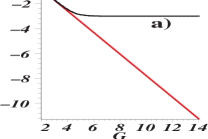
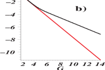
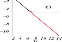
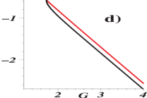
Figure 4: Logarithmic plot of minimum phase spread $\log_{10}(\delta\varphi)$ determined from (8) (curved black lines) and of four times the inverse intensity $\log_{10}(4/(2\sinh(G)^{2}))$ (straight red lines) comparing various loss mechanisms: a) $\alpha_{1}=\beta_{1}=\pi/300$, b) $\alpha_{2}=\beta_{2}=\pi/300$, c) $\Delta_{1}=1/300000$, d) $\Delta_{2}=-1/3$. Note the different orders of magnitude in the values of $\Delta_{1}$ and $\Delta_{2}$ and the fact that ’d)’, surprisingly, shows a slight improvement in performance for a large negative imbalance $\Delta_{2}=-1/3$.

FIG. 4 compares the various cases for losses and imbalances and shows that the system is more forgiving for losses in the interferometer part than in the state preparation part: the utilized quantum state has to be prepared with great skill but the scheme is comparatively robust to imperfections of the interferometer. When all imperfections are studied simultaneously their effects add up, i.e., tend to be dominated by the largest effect(s).

Let us first consider losses in the state preparation part of the setup, i.e. losses in modes $\hat{a}_{1}$ and $\hat{b}_{1}$ extending from inside the crystal to the first beam-splitter ${\sf B}_{1}$. They are described by the mode-transformations $\hat{a}_{1}\mapsto\cos(\alpha_{1})\hat{a}_{1}+\sin(\alpha_{1})\hat{u}_{1}$ and $\hat{b}_{1}\mapsto\cos(\beta_{1})\hat{b}_{1}+\sin(\beta_{1})\hat{v}_{1}$ plus subsequent tracing over the loss modes (not mentioned) and the admixed vacuum modes $\hat{u}_{1}$ and $\hat{v}_{1}$. It turns out that the qualitative picture does not depend much on the details such as whether the loss parameters $\alpha_{1}$ and $\beta_{1}$ are equal or the losses occur in one channel only. Thus, with experiments in mind, let us assume symmetric losses, namely $\alpha_{1}=\beta_{1}=\pi/300\approx 0.01$ leading to $0.0001=0.01$ % losses in both channels. For example, mode-mismatch at the beam splitter ${\sf B}_{1}$ leads to such symmetrical admixture of vacuum. This scheme is very sensitive to losses in the state preparation part of the setup and shows saturation of performance, see FIG. 4 a): to gain an order of magnitude in performance $\alpha_{1}$ and $\beta_{1}$ have to be decreased by half an order of magnitude, namely, $\delta\varphi$ saturates at about $9\alpha_{1}^{2}$.

Losses in the interferometric part of the setup (modes $\hat{a}_{2}$ and $\hat{b}_{2}$) are analogously described by loss parameters $\alpha_{2}$ and $\beta_{2}$ which parameterize the admixture of two more vacuum modes $\hat{u}_{2}$ and $\hat{v}_{2}$ to the path modes $\hat{a}_{2}$ and $\hat{b}_{2}$. FIG. 4 b) illustrates the greater tolerance of our scheme to losses in the interferometer part of the setup. For the same loss values, $\alpha_{2}=\beta_{2}=\pi/300$ as for $\alpha_{1}$ and $\beta_{1}$ before, the scheme shows a relatively better performance, indeed, the performance does not show saturation at all. Instead, at the threshold intensity $\approx 4/(9\alpha^{2})$ it switches from $\delta\varphi\approx 4/\langle N\rangle$ to the poorer scaling $\delta\varphi=\kappa/\sqrt{\langle N\rangle}$, maintaining the ground it has gained. Namely, beyond the threshold intensity we find $\delta\varphi\approx 6\,|\alpha_{2}|/\sqrt{\langle N\rangle}$.

Analogously to the case of losses, the scheme is also much more sensitive to imbalances of the first beam-splitter ${\sf B}_{1}$ than to those of ${\sf B}_{2}$, which is described by

$$\hat{\sf B}_{2}\left[\begin{array}[]{cc}\hat{a}_{2}\\ \hat{b}_{2}\end{array}\right]=\left[\begin{array}[]{lr}-\cos(\frac{\pi}{4}+\Delta_{2})&i\sin(\frac{\pi}{4}+\Delta_{2})\\ \vskip 6.0pt plus 2.0pt minus 2.0pt\cr-i\sin(\frac{\pi}{4}+\Delta_{2})&\cos(\frac{\pi}{4}+\Delta_{2})\end{array}\right]\left[\begin{array}[]{cc}\hat{a}_{2}\\ \hat{b}_{2}\end{array}\right]$$ (15)

conforming with the case $\Delta_{2}=0$ used in the derivation of Eqs. (2) and (3). The imbalance in transformation $\hat{\sf B}_{1}$ is described, in full analogy, by an imbalance angle $\Delta_{1}$. Similarly to the case of $\alpha_{1}$ a non-zero $\Delta_{1}$ leads to saturation: for positive imbalances the saturation level is $\delta\varphi\approx 4\Delta_{1}$ and it is $\delta\varphi\approx 12|\Delta_{1}|$ for negative $\Delta_{1}$.

It turns out that variation of $\Delta_{2}$ modifies the coefficient $\kappa$ but not the scaling exponent in $\delta\varphi=\kappa/\langle N\rangle$; as mentioned above, for $\Delta_{2}=0$ we find $\delta\varphi=4/\langle N\rangle$. Note that, surprisingly, a large (negative) imbalance $\Delta_{2}$, as is displayed in FIG. 4 d), yields a small increase in performance quality ($\kappa$ is being reduced). I cannot explain this finding and I think it deserves further investigation and might even lead to a trick to reduce the scaling reported here down to the Heisenberg-limit $\delta\varphi=1/\langle N\rangle$. Variation of the value of the imbalance parameter $\Delta_{2}$ alone, leads to an optimal value for the imbalance of approximately $\Delta_{2}\approx-0.2375\hat{=}-13.61^{o}$ and to our central result Eq. (1). This probably is the best our scheme can offer.

Over recent years a consensus has emerged that a sharp photon number distribution is needed to reach the Heisenberg-limit Sanders95 ; Dowling98 ; Gerry02 ; Soederholm.0204031 . It was therefore even concluded that the perceived need of a sub-poissonian photon number distribution renders the two-mode squeezed vacuum state unsuitable for interferometry because of its super-poissonian thermal photon number distribution Sanders95 ; Gerry02 ; in the light of these claims our central result Eq. (1) is rather surprising.

Note, that we did not discuss a criterion for the power of the pump beam driving the parametric down-conversion source and of the power needed for the strong local oscillator fields necessary to perform the balanced homodyne measurements H_a and H_b, see FIG. 1. If this is included, the effective performance of our scheme could be reclassified as less efficient, yet, it remains a scheme with Heisenberg-limit–like scaling. The penalty to pay is not too large for large intensities because the local oscillator’s shot-noise-to-signal-ratio diminishes with increasing signal strength thus yielding very accurate homodyning signals. In this context I would also like to mention that there are promising recent ideas for efficient and bright down-conversion sources DeRossi02 .

Also note, that the considerations of this paper might turn out to be of importance for atom-beam interferometry Dowling98 since four-wave mixing has been reported yielding correlated atom beams in states similar to the two-mode squeezed vacuum states discussed here Vogels02 .

Conclusions: We have found that bosonic two-mode squeezed states can be used in an interferometer to achieve phase resolution near the Heisenberg-limit, see Eq. (1). This only works at particular phase settings, the noise is phase sensitive and the setup therefore needs a feedback mechanism. The degrading influence of experimental imperfections is analyzed and it is shown that requirements on the state-preparation part of the setup are very stringent. On the other hand our scheme is more robust with respect to imperfections of the interferometer part of the setup and it does not suffer from single-photon detection problems because it relies on balanced homodyne-detection.

- (1) M. O. Scully and M. S. Zubairy, Quantum Optics, (Cambridge Univ. Press, Cambridge, 1997).
- (2) C. M. Caves, Phys. Rev. Lett. 45, 75 (1980).
- (3) C. M. Caves, Phys. Rev. D 23, 1693 (1981).
- (4) R. S. Bondurant and J. H. Shapiro, Phys. Rev. D 30, 2548 (1984).
- (5) B. Yurke, S. L. McCall, and J. R. Klauder, Phys. Rev. A 33, 4033 (1986).
- (6) M. Xiao, L.-A. Wu, and H. J. Kimble, Phys. Rev. Lett. 59, 278 (1987).
- (7) P. Grangier, R. E. Slusher, B. Yurke, and A. LaPorta, Phys. Rev. Lett. 59, 2153 (1987).
- (8) M. J. Holland and K. Burnett, Phys. Rev. Lett. 71, 1355 (1993).
- (9) M. Hillery and L. Mlodinow, Phys. Rev. A 48, 1548 (1993).
- (10) J. Jacobson, G. Björk, I. Chuang, and Y. Yamamoto, Phys. Rev. Lett. 74, 4835 (1995).
- (11) B. C. Sanders and G. J. Milburn, Phys. Rev. Lett. 75, 2944 (1995).
- (12) Z. Y. Ou, Phys. Rev. Lett. 77, 2352 (1996); Phys. Rev. A 55, 2598 (1997).
- (13) C. Brif and A. Mann, Phys. Rev. A 54, 4505 (1996).
- (14) T. Kim, O. Pfister, M. J. Holland, J. Noh, and J. L. Hall, Phys. Rev. A 57, 4004 (1998).
- (15) J. Dowling, Phys. Rev. A 57, 4736 (1998).
- (16) C. C. Gerry and A. Benmoussa, Phys. Rev. A 65, 033822 (2002).
- (17) J. Söderholm et al., quant-ph/0204031.
- (18) D. T. Smithey, M. Beck, M. G. Raymer, and A. Faridani, Phys. Rev. Lett. 70 1244 (1993).
- (19) D. T. Smithey, M. Beck, M. Belsley, and M. G. Raymer, Phys. Rev. Lett. 69, 2650 (1992).
- (20) A. Lamas-Linares, J. C. Howell, and D. Bouwmeester, Nature 412, 887 (2001).
- (21) G. S. Agarwal, R. W. Boyd, E. M. Nagasako, and S. J. Bentley, Phys. Rev. Lett. 86, 1389 (2001).
- (22) C. W. Gardiner and P. Zoller, Quantum Noise, (Springer, Berlin, 2000).
- (23) A. De Rossi and V. Berger, Phys. Rev. Lett. 88, 043901 (2002).
- (24) J. M. Vogels, K. Xu, and W. Ketterle, Phys. Rev. Lett. 89, 020401 (2002); L. Deng et al., Nature (London) 398, 218 (1999).