Driving non-Gaussian to Gaussian states with linear optics

Abstract

We introduce a protocol that maps finite-dimensional pure input states onto approximately Gaussian states in an iterative procedure. This protocol can be used to distill highly entangled bi-partite Gaussian states from a supply of weakly entangled pure Gaussian states. The entire procedure requires only the use of passive optical elements and photon detectors that solely distinguish between the presence and absence of photons.

I Introduction

Gaussian entangled states may be prepared quite simply in optical systems: one only has to mix a pure squeezed state with a vacuum state at a beam splitter, both of which are special instances of Gaussian states in systems with canonical coordinates generation ; Gauss . The beam splitter acts as a Gaussian unitary operation which modifies the quantum state, but does not alter the Gaussian character of the state. The resulting pure state is a two-mode squeezed state. This state may be used as the resource for protocols in quantum information processing. In fact, teleportation teleportation , dense coding densecoding and cryptographic schemes cryptography on the basis of such two-mode squeezed states have been either studied theoretically or already experimentally realised. For the theory of quantum information processing in systems with canonical degrees Gaussian states play a role closely analogous to that of entangled states of qubits, for which most of the theory of quantum information processing has been developed.

However, there are significant limits to what accuracy highly entangled two-mode squeezed states may be prepared and distributed over large distances. Firstly, the degree of single-mode squeezing that can be achieved limits the degree of two-mode squeezing of the resulting state. Secondly, decoherence is unavoidable in the transmission of states through fibres, and the original highly entangled state will deteriorate into a very weakly entangled mixed Gaussian state Stefan . For finite-dimensional systems, it has been one of the key observations that in fact, from weakly entangled states one can obtain highly entangled states by means of local quantum operations supported by classical communication Bennett at the price of starting from a large number of weakly entangled systems but ending with a smaller number of more strongly entangled systems. The term entanglement distillation has been coined for such procedures. Importantly, such methods function also as the basis for security proofs of quantum cryptographic schemes HansHans .

It was generally expected that an analogous procedure should exists for the distillation of Gaussian states by means of local Gaussian operations and classical communication only. Surprisingly however, it was recently proven that this is not the case Dist ; Dist2 . For example, no matter how the local Gaussian quantum operations are chosen, one cannot map a large number of weakly entangled two-mode squeezed states onto a single highly entangled Gaussian state. Gaussian quantum operations Dist ; Dist2 ; operations correspond in optical systems to the application of optical elements such as beam splitters, phase shifts and $\chi^{(2)}$-squeezers, together with homodyne detection. All these operations are, to some degree of accuracy, experimentally accessible. With non-Gaussian quantum operations, in turn, one can distill finite-dimensional states out of a supply of Gaussian states Duan , but the resulting states are not Gaussian, and the experimental implementation of the known protocols constitutes a significant challenge.

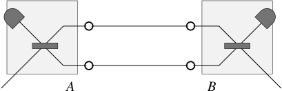
Figure 1: A single step of the protocol. Two pairs of entangled two-mode states are mixed locally at 50:50 beam splitters and absence or presence of photons is detected in one of the output arms on both sides.

One may be tempted to think that this observation renders all attempts to increase the degree of entanglement in Gaussian states impossible. In this article, however, we discuss the possibility of obtaining a Gaussian state with arbitrarily high fidelity from a supply of non-Gaussian states employing only Gaussian operations, namely linear optical elements and projections onto the vacuum. We describe a protocol that prepares approximate Gaussian states from a supply of non-Gaussian states, which shall be called ’Gaussification’ from now on. The non-Gaussian states that we use could in particular be obtained from weakly two-mode squeezed vacua, by the application of a beam splitter and a photon detector. Together with this step, the proposed procedure offers a complete distillation procedure of Gaussian states to (almost exact) Gaussian states, but via non-Gaussian territory. It is important to note that the protocol introduced below is by no means restricted to a bi-partite setting. The bi-partite case is only practically the most important one, as it allows in effect for distillation of Gaussian states with non-Gaussian operations. But this method can, in particular, also be used in a mono-partite setting to approximately obtain a Gaussian state from a supply of unknown non-Gaussian states.

The paper is organised as follows: First, we will describe the protocol, that generates Gaussian states from a supply of non-Gaussian states. This protocol requires only passive optical elements and photon detectors that can distinguish between the absence or presence of photons but that do not determine their exact number. We then proceed by discussing the effect of the protocol in more detail. We will discuss the special case of pure states in Schmidt form as well as general pure states. The fixed points of the iteration map will be identified as pure Gaussian states and a proof of convergence will be given. Finally, we will discuss the feasible preparation of finite-dimensional states from a supply of pure Gaussian states.

II The protocol

The protocol is very simple indeed. We start with a supply of identically prepared bi-partite non-Gaussian states. The overall protocol then amounts to an iteration of the following basic steps:

1. The states will be mixed pairwise locally at 50:50 beam splitters (see Fig. 1).

2. On one of the outputs of each beam splitter a photon detector distinguishes between the absence and presence of photons. It should be noted that we do not require photon counters that can discriminate between different photon numbers.

3. In case of absence of photons at both detectors for a particular pair one keeps the remaining modes as an input for the next iteration, otherwise the state is discarded.

This is one iteration of the protocol which we will continue until we finally end up with a small number of states that closely resemble Gaussian states. This is clearly a probabilistic protocol. However, the success probability, as we will see later, can be quite high. It should also be noted that the operations in a successful run are indeed Gaussian operations, namely the use of linear optical elements and vacuum projections. Each of these steps can be realised with present-day technology.

III Examples of the protocol

III.1 Pure states in Schmidt form

In order to demonstrate the general mechanism, we start by discussing a particularly simple case, namely pure states in Schmidt form. We do not require any prior knowledge of the actual un-normalised state vectors except that they can be expressed in the following form

$$|\psi^{(0)}\rangle=\sum_{n=0}^{\infty}\alpha_{n,n}^{(0)}|n,n\rangle,$$ (1)

where $\{\alpha_{n,n}^{(0)}\}_{n=0}^{\infty}$ with $\alpha_{n,n}^{(0)}\!\geq\!0$ are proportional to the real Schmidt coefficients of the state vector, and $\{|n\rangle:n\in{\mathbb{N}}\}$ denotes the Fock basis. We only assume $\alpha_{0,0}^{(0)}\!>\!0$ and it is then convenient to consider un-normalized states for which we set $\alpha_{0,0}^{(0)}\!=\!1$. The un-normalized states arising in later steps $i\!=\!1,2,\ldots$ are characterised by coefficients $\{\alpha_{n,n}^{(i)}\}_{n=0}^{\infty}$. These coefficients then become identical to the Schmidt coefficients only after appropriate normalisation. Starting from two identical copies of state vectors that have been obtained in the $i$th step of the protocol , i.e.

$$|\psi^{(i)}\rangle|\psi^{(i)}\rangle$$ (2)

one obtains after application of the 50:50 beam splitters the state vector $(\hat{U}_{12}\otimes\hat{U}_{12})|\psi^{(i)}\rangle|\psi^{(i)}\rangle$. Here, the beam splitter is described by (see, e.g., vogelwelsch )

$$\hat{U}_{12}=T^{\hat{n}_{1}}e^{-R^{\ast}\hat{a}_{2}^{\dagger}\hat{a}_{1}}e^{R\hat{a}_{2}\hat{a}_{1}^{\dagger}}T^{-\hat{n}_{2}}\,,$$ (3)

where $\hat{U}_{12}$ acts on the amplitude operators of the field modes as

$$\hat{U}_{12}\left(\begin{array}[]{c}\hat{a}_{1}\\ \hat{a}_{2}\end{array}\right)\hat{U}_{12}^{\dagger}=\left(\begin{array}[]{cc}T&R\\ -R^{\ast}&T^{\ast}\end{array}\right)\left(\begin{array}[]{c}\hat{a}_{1}\\ \hat{a}_{2}\end{array}\right)$$ (4)

where we set $T\!=\!R\!=\!1/\sqrt{2}$. The resulting un-normalised state vector, conditional on vacuum outcomes in both detectors, is given by

$$|\psi^{(i+1)}\rangle := \langle 0,0|(\hat{U}_{12}\otimes\hat{U}_{12})|\psi\rangle|\psi\rangle$$ (5)

$$= \sum_{n=0}^{\infty}\left[2^{-n}\sum_{r=0}^{n}{n\choose r}\alpha_{r,r}^{(i)}\alpha_{n-r,n-r}^{(i)}\right]|n,n\rangle$$

$$= \sum_{n=0}^{\infty}\alpha_{n,n}^{(i+1)}|n,n\rangle,$$

where

$$\alpha_{n,n}^{(i+1)}:=2^{-n}\sum_{r=0}^{n}{n\choose r}\alpha_{r,r}^{(i)}\alpha_{n-r,n-r}^{(i)}$$ (6)

for $n=0,1,\ldots$.The probability of vacuum outcomes being detected in both modes is $\langle\psi^{(i+1)}|\psi^{(i+1)}\rangle/\lvert\langle\psi^{(i)}|\psi^{(i)}\rangle\rvert^{2}$. The protocol is a Gaussian quantum operation, in the sense that it is a completely positive map that maps all Gaussian states onto Gaussian states. The interesting feature is that by repeated application it also maps non-Gaussian states arbitrarily close to Gaussian states, as will be demonstrated below.

In effect, in each iteration one maps one sequence of coefficients $\alpha^{(i)}\!=\!\{\alpha_{n,n}^{(i)}\}_{n=0}^{\infty}$ onto another sequence $\alpha^{(i+1)}\!=\!\{\alpha_{n,n}^{(i+1)}\}_{n=0}^{\infty}$, defining the map $\Phi$ via

$$\alpha^{(i+1)}=:\Phi(\alpha^{(i)})\,.$$ (7)

In the following we use the notation $\Phi^{(1)}\!=\!\Phi$ and $\Phi^{(i+1)}\!=\!\Phi\circ\Phi^{(i)}$ for $i=0,1,...$. The main observation is that in fact, provided $\alpha_{1,1}^{(0)}\!<\!\alpha_{0,0}^{(0)}$, the sequence of coefficients $\{\alpha^{(i)}\}_{i=1}^{\infty}$ converges to a distribution corresponding to a Gaussian state, in this special case a two-mode squeezed vacuum.

In other words, although the initial state was not Gaussian, but say, a state corresponding to a finite-dimensional state vector of the form

$$|\psi^{(0)}\rangle=|0,0\rangle+\alpha_{1,1}^{(0)}|1,1\rangle,$$ (8)

where $\alpha_{1,1}^{(0)}\in[0,1)$, after a number of steps the resulting state is Gaussian to a high degree of accuracy. We will first show that this convergence is a general feature of this protocol, and we will then discuss the consequences. We start by demonstrating that those distributions associated with pure Gaussian states are fixed points of the map $\Phi$.

Proposition 1. – The distributions $\alpha=\{\alpha_{n,n}\}_{n=0}^{\infty}$ of the form

$$\alpha_{n,n}=\lambda^{n},$$ (9)

$\lambda\geq 0$, corresponding to two-mode squeezed states, are the only fixed points of the map $\Phi$.

Proof. This can be immediately derived from the definition of $\Phi$: Let us assume that

$$\alpha\!=\!\Phi(\alpha)$$ (10)

holds. It can be verified by substitution that $\alpha_{n,n}=\lambda^{n}$ is a solution of this equation. The uniqueness of this solution can be verified by observing that Eq. (10) also implies $\alpha_{0,0}\!=\!\alpha_{0,0}^{2}$, that is, $\alpha_{0,0}\!=\!1$. Then $\alpha_{1,1}$ is a free parameter and once set (i.e. as $\alpha_{1,1}=\lambda$) the remaining coefficients are uniquely determined.

These coefficients, for $\lambda\in[0,1)$, in turn correspond exactly to two-mode pure Gaussian states. If $\lambda$ lies outside this range, the state is not normalizable. The next Proposition states that those distributions associated with Gaussian states are not only fixed points of the map $\Phi$, but provided $\alpha_{0,0}^{(0)}\!\neq\!0$, each sequence of coefficients converges to such a fixed point.

Proposition 2. – Let $\alpha^{(0)}\!=\!\{\alpha_{n,n}^{(0)}\}_{n=0}^{\infty}$ with $a_{0,0}^{(0)}=1$ and $0\!\leq\!\alpha_{1,1}^{(0)}\!<\!1$. Then

$$\lim_{i\rightarrow\infty}\alpha^{(i)}_{n,n}=\alpha^{(\infty)}_{n,n}$$ (11)

for all $n=0,1,...$, where $\alpha^{(\infty)}$ is a distribution of the type of Proposition 1.

Proof. As before, let us set $\alpha^{(i)}\!:=\!\Phi^{(i)}(\alpha^{(0)})$ for $i\!=\!1,2,\ldots$. The first step is to see that

$$\frac{\alpha_{1,1}^{(i+1)}}{\alpha_{0,0}^{(i+1)}}=\frac{\alpha_{1,1}^{(i)}}{\alpha_{0,0}^{(i)}}=\alpha_{1,1}^{(0)}$$ (12)

for all $i\!=\!0,1,\ldots$. Let us first assume that $\alpha_{1,1}^{(0)}>0$. Then, as can be seen from the definition of $\Phi$,

$$\alpha_{2,2}^{(i+1)}\alpha_{1,1}^{(i)}=\frac{1}{2}\left(\alpha_{2,2}^{(i)}+\alpha_{1,1}^{(0)}\alpha_{1,1}^{(i)}\right)\alpha_{1,1}^{(i+1)}.$$ (13)

Hence, as $\alpha_{1,1}^{(i)}=\alpha_{1,1}^{(0)}>0$ for all $i=0,1,...$,

$$\lim_{i\rightarrow\infty}\frac{\alpha_{2,2}^{(i)}}{\alpha_{1,1}^{(i)}}=\alpha_{1,1}^{(0)}.$$ (14)

Now let us assume that already $\alpha_{n-1,n-1}^{(i)}>0$ for all $i=0,1,...$ and

$$\lim_{i\rightarrow\infty}\frac{\alpha_{n,n}^{(i)}}{\alpha_{n-1,n-1}^{(i)}}=\alpha_{1,1}^{(0)}$$ (15)

for some $n\!=\!1,2,\ldots$. Then, from

$$\frac{\alpha_{n+1,n+1}^{(i+1)}}{\alpha_{n,n}^{(i+1)}} = \frac{1}{2}\frac{\sum_{r=0}^{n+1}\alpha_{r,r}^{(i)}\alpha_{n-r+1,n-r+1}^{(i)}{n+1\choose r}}{\sum_{r=0}^{n}\alpha_{r,r}^{(i)}\alpha_{n-r,n-r}^{(i)}{n\choose r}}$$ (16)

it follows after a few steps that $a_{n,n}^{(i)}>0$ for all $i=0,1,...$, and

$$\begin{split}&\lim_{i\rightarrow\infty}\frac{\alpha_{n+1,n+1}^{(i+1)}}{\alpha_{n,n}^{(i+1)}}=\\ &\lim_{i\rightarrow\infty}\frac{1}{2^{n+1}}\left[\frac{2\alpha_{n+1,n+1}^{(i)}}{\alpha_{n,n}^{(i)}}+(2^{n+1}-2)\alpha_{1,1}^{(0)}\right],\end{split}$$ (17)

which means that

$$\lim_{i\rightarrow\infty}\frac{\alpha_{n+1,n+1}^{(i+1)}}{\alpha_{n,n}^{(i+1)}}=\alpha_{1,1}^{(0)}.$$ (18)

Hence, by induction we find that the ratios of $\alpha_{n+1,n+1}^{(i)}$ and $\alpha_{n,n}^{(i)}$ converge to the ratio of $0\!<\!\alpha_{1,1}^{(0)}\!<\!1$ and $\alpha_{0,0}^{(0)}\!=\!1$ as $i\!\to\!\infty$. This means that the coefficients correspond to a Gaussian state as specified in Proposition 1. In case that $\alpha_{1,1}^{(0)}=0$ an analogous argument can be applied in order to arrive at $\alpha_{0,0}^{(i)}=1$ for all $i=0,1,...$ and

$$\lim_{i\rightarrow\infty}\alpha_{n,n}^{(i)}=0$$ (19)

for all $n\!=\!1,2,\ldots$.

This shows formally that the (pointwise) convergence to an effectively Gaussian state is generic Gen . Putting aside the restriction that $\alpha_{0,0}^{(0)}=1$, three cases shall be discussed in more detail.

1. If $\alpha_{0,0}^{(0)}\!>\!0$ and $\alpha_{1,1}^{(0)}\!<\!\alpha_{0,0}^{(0)}$, then the states converge to a Gaussian state.

2. A special instance is when $\alpha_{0,0}^{(0)}\!>\!0$, but $\alpha_{1,1}^{(0)}\!=\!0$. Then the states converge to a Gaussian state, but to the product of two vacua.

3. If $\alpha_{0,0}^{(0)}\leq\alpha_{1,1}^{(0)}$, then the sequence does not converge to a sequence of coefficients corresponding to a Gaussian state. In particular, this is always the case when

   $$\alpha_{0,0}^{(0)}\!=\!0.$$ (20)

   This follows immediately from Eq. (6) as $\alpha_{0,0}^{(i)}\!=\!0$ for all $i$.

In practice, one can actually expect a state that is very close to a Gaussian state already after a very small number of steps, say, three or four steps. As has already been mentioned, the whole scheme is probabilistic. That is, the success probability of actually obtaining the desired state is always less than one. In Fig. 2 we show the total probability of success, $p_{\text{success}}^{(i)}$, and in Fig. 3 the corresponding fidelity $F^{(i)}$, i.e. the overlap with the Gaussian state to which the protocol converges, after $i\!=\!1,2,3$ iteration steps. Here, we started with coefficients $\alpha_{0,0}^{(0)}\!=\!1$ and $\alpha_{1,1}^{(0)}\!=\!\lambda$.

Figure 2: Success probability $p_{\text{success}}^{(i)}$ after $i\!=\!1$ (dotted line), $i\!=\!2$ (dashed line) and $i\!=\!3$ (solid line) iteration steps, where the initial states were $\propto|0,0\rangle+\lambda|1,1\rangle$.

Figure 3: Fidelity $F^{(i)}$ of the approximately Gaussian state after $i\!=\!1$ (dotted line), $i\!=\!2$ (dashed line) and $i\!=\!3$ (solid line) iterations where the initial states were $\propto|0,0\rangle+\lambda|1,1\rangle$.

We see that for a large range of values for $\lambda$ the fidelity is just below unity, and for $\lambda\!=\!0.5$ the probability of success is still above 0.5.

III.2 General pure states

Suppose now we have a supply of pure states with state vectors of the general form

$$|\psi^{(0)}\rangle=\sum_{m,n=0}^{\infty}\alpha^{(0)}_{m,n}|{m,n}\rangle,$$ (21)

where $\alpha^{(0)}_{m,n}\in{\mathbbm{C}}$ for all $n,m$. If the procedure described in Sec. II is carried out, using 50:50 beam splitters with appropriate phases, such that $T\!=\!R\!=\!1/\sqrt{2}$, then, for a large class of input states, after repeated iterations of the protocol, a state closely approximating a Gaussian state will be obtained. If the identical retained states after $i$ iterations of the procedure are labeled

$$|\psi^{(i)}\rangle\!=\!\sum_{m,n}\alpha^{(i)}_{m,n}|m,n\rangle,$$ (22)

we can describe each iteration in terms of the following recurrence relation,

$$\begin{split}\alpha_{m,n}^{(i)}\longmapsto\alpha_{m,n}^{(i+1)}&=2^{-\frac{m+n}{2}}\sum_{r=0}^{m}\sum_{s=0}^{n}(-1)^{(m+n)-(r+s)}\\ &\times\alpha_{r,s}^{(i)}\alpha_{m-r,n-s}^{(i)}\left[{{m\choose r}{n\choose s}}\right]^{1/2},\end{split}$$ (23)

where again

$$\alpha^{(i+1)}=\Phi(\alpha^{(i)}),$$ (24)

with $\alpha^{(i)}=\{\alpha^{(i)}_{n,m}\}_{n,m=0}^{\infty}$ for $i=0,1,...$. We will in the following write

$$\alpha_{n,m}^{(\infty)}:=\lim_{i\rightarrow\infty}\alpha_{n,m}^{(i)},$$ (25)

whenever this limit exists. The fixed points of $\Phi$, characterised by $\alpha_{m,n}^{(\infty)}\in{\mathbbm{C}}$, correspond to states which are unchanged by one or more iterations of the procedure, and satisfy $\Phi(\alpha^{(\infty)})\!=\!\alpha^{(\infty)}$, thus

$$\begin{split}\alpha_{m,n}^{(\infty)}&=2^{-\frac{m+n}{2}}\sum_{r=0}^{m}\sum_{s=0}^{n}(-1)^{(m+n)-(r+s)}\\ &\times\alpha_{r,s}^{(\infty)}\alpha_{m-r,n-s}^{(\infty)}\left[{{m\choose r}{n\choose s}}\right]^{1/2}\end{split}$$ (26)

for all $n,m$. We immediately see that

$$\alpha_{0,0}^{(\infty)}\!=\!(\alpha_{0,0}^{(\infty)})^{2}$$ (27)

and thus $\alpha_{0,0}^{(\infty)}\!=\!1$. (The other possibility, $\alpha_{0,0}^{(\infty)}\!=\!0$ leads to the trivial solution $\alpha_{m,n}^{(\infty)}\!=\!0$ for all $m,n$.) We also find that the coefficients $\alpha_{1,1}^{(\infty)}$, $\alpha_{2,0}^{(\infty)}$ and $\alpha_{0,2}^{(\infty)}$ are the only free parameters. When these values are specified, all other coefficients are determined. The general solution of Eq. (26) is

$$\alpha_{2m,2n+1}^{(\infty)}=\alpha_{2m+1,2n}^{(\infty)}=0\,,$$ (28)

$$\alpha_{2m,2n}^{(\infty)}=\sqrt{(2m)!}\sqrt{(2n)!}$$ (29)

$$\times\sum_{0\leq s\leq m;s\leq n}\left[\frac{\gamma_{12}^{2s}}{(2s)!}\frac{\left(\gamma_{1}/{2}\right)^{m-s}}{(m-s)!}\frac{\left(\gamma_{2}/{2}\right)^{n-s}}{(n-s)!}\right]\,,$$

$$\alpha_{2m+1,2n+1}^{(\infty)}=\sqrt{(2m+1)!}\sqrt{(2n+1)!}$$ (30)

$$\times\sum_{0\leq s\leq m;s\leq n}\left[\frac{\gamma_{12}^{2s+1}}{(2s+1)!}\frac{\left(\gamma_{1}/{2}\right)^{m-s}}{(m-s)!}\frac{\left(\gamma_{2}/{2}\right)^{n-s}}{(n-s)!}\right]\,,$$

where the coefficients $\gamma_{1},\gamma_{2}$ and $\gamma_{12}$ are usefully expressed as elements of the symmetric $2\times 2$ matrix

$$\bm{\Gamma}=\left(\begin{array}[]{cc}\gamma_{1}&\gamma_{12}\\ \gamma_{12}&\gamma_{2}\end{array}\right)$$ (31)

and are determined uniquely by the free parameters $\alpha_{2,0}^{(\infty)},\alpha_{0,2}^{(\infty)}$ and $\alpha_{1,1}^{(\infty)}$. A specific form for this correspondence is given in Proposition 4. The coefficients $\alpha_{mn}^{(\infty)}$ determine an un-normalized state vector $|\psi(\bm{\Gamma})\rangle$. In the Fock state representation this state vector is given by

$$|\psi(\bm{\Gamma})\rangle=\hat{Q}(\bm{\Gamma})|0,0\rangle,$$ (32)

where the operator $\hat{Q}(\bm{\Gamma})$ is expressed in terms of $\bm{\Gamma}$ and the vector $\hat{\bm{a}}^{\dagger}\!=\!(\hat{a}^{\dagger}_{1},\hat{a}^{\dagger}_{2})^{T}$ as

$$\hat{Q}(\bm{\Gamma})=\exp\left[\frac{1}{2}(\hat{\bm{a}}^{\dagger})^{T}\bm{\Gamma}(\hat{\bm{a}}^{\dagger})\right]\,.$$ (33)

The state vectors $|\psi(\bm{\Gamma})\rangle$ are not normalized, and the requirement that they be normalizable, i.e. $\langle\psi(\bm{\Gamma})|\psi(\bm{\Gamma})\rangle$ is finite, places a restriction on $\bm{\Gamma}$. The following proposition takes its most concise form when we use the spectral norm which is defined as Horn

$$\lvert\lvert\bm{X}\rvert\rvert_{\infty}=\sqrt{\lambda_{\text{max}}}$$ (34)

where $\lambda_{\text{max}}$ is the largest eigenvalue of $\bm{X}\bm{X}^{\dagger}$.

Proposition 3. – If and only if $\lvert\lvert\bm{\Gamma}\rvert\rvert_{\infty}\!<\!1$, then $|\psi(\bm{\Gamma})\rangle\!:=\!\hat{Q}(\bm{\Gamma})|0,0\rangle$ is normalizable and represents a pure Gaussian state.

Proof: The matrix $\bm{\Gamma}$ in Eq. (31) is a complex symmetric $2\times 2$-matrix. Following Takagi’s Lemma Horn , there exists a unitary matrix $\bm{U}$ such that

$$\bm{U}^{T}\bm{\Gamma}\bm{U}\!=:\!\bm{\Delta},$$ (35)

where $\bm{\Delta}$ is a diagonal matrix the entries of which are the eigenvalues of $\sqrt{\bm{\Gamma}\bm{\Gamma}^{\dagger}}$. With $\hat{\bm{b}}\!:=\!\bm{U}\hat{\bm{a}}$ we have

$$|\psi(\bm{\Gamma})\rangle=\exp\left[\frac{1}{2}(\hat{\bm{b}}^{\dagger})^{T}\bm{\Delta}(\hat{\bm{b}}^{\dagger})\right]|0,0\rangle\,.$$ (36)

Because the $\hat{b}_{1}$ and $\hat{b}_{2}$ commute, this is a tensor product of two single-mode Gaussian states. It is now straightforward to show that the single mode state vectors are normalizable if and only if both diagonal elements of $\bm{\Delta}$ are smaller than one. Then, each of the modes is in a single-mode squeezed state Ma90 . The transformation $\hat{\bm{a}}\!\longmapsto\!\bm{U}\hat{\bm{a}}$ represents a beam-splitter transformation mapping the original modes $\hat{\bm{a}}$ onto the modes $\hat{\bm{b}}$, i.e. it is a passive transformation. Hence, the resulting state vector Eq. (32) is also normalizable.

In fact, as can be shown, the state vector $\hat{Q}(\bm{\Gamma})|0,0\rangle$ is, apart from normalisation, equal to the state vector of the two-mode squeezed vacuum state $\hat{S}(\bm{Z})|0,0\rangle$, where

$$\hat{S}(\bm{Z})=\exp\left[\frac{1}{2}(\hat{\bm{a}}^{\dagger})^{T}\bm{Z}(\hat{\bm{a}}^{\dagger})-\frac{1}{2}(\hat{\bm{a}})^{T}\bm{Z}^{\dagger}(\hat{\bm{a}})\right]\,.$$ (37)

$\hat{S}(\bm{Z})$ is a generalized two-mode squeezing operator Ma90 ,

$$\bm{Z}=-\left(\begin{array}[]{cc}\zeta_{1}&\zeta_{12}\\ \zeta_{12}&\zeta_{2}\end{array}\right),$$ (38)

where $\bm{Z}\!=\!\mbox{\rm arctanh}(\bm{r_{\Gamma}})e^{i\bm{\theta_{\Gamma}}}$ with the polar decomposition

$$\bm{\Gamma}\!=\!\bm{r_{\Gamma}}e^{i\bm{\theta_{\Gamma}}}.$$ (39)

Proposition 4. – Suppose we are given a supply of identical two-mode pure states with state vectors $|\psi^{(0)}\rangle\!=\!\sum_{m,n}\alpha_{m,n}^{(0)}|m,n\rangle$, and let

$$\bm{\Gamma}:=\left(\begin{array}[]{cc}\sqrt{2}\beta_{2,0}-\beta_{1,0}^{2}&\beta_{1,1}-\beta_{1,0}\beta_{0,1}\\ \beta_{1,1}-\beta_{1,0}\beta_{0,1}&\sqrt{2}\beta_{0,2}-\beta_{0,1}^{2}\end{array}\right),$$ (40)

where $\beta_{m,n}\!:=\!\alpha_{m,n}^{(0)}/\alpha_{0,0}^{(0)}$. If $\lvert\lvert\bm{\Gamma}\rvert\rvert_{\infty}\!<\!1$ then

$$\lim_{i\rightarrow\infty}\alpha_{m,n}^{(i)}=\alpha_{m,n}$$ (41)

for all $n,m=0,1,...$, where

$$\alpha_{m,n}:=\langle m,n|\hat{Q}(\bm{\Gamma})|0,0\rangle.$$ (42)

Proof. To make the proof simpler, we shall use $\alpha_{0,0}^{(0)}\!=\!1$ as above. This is merely a change of normalization and does not alter the general validity of the argument. Before proving the convergence of all coefficients $\alpha_{m,n}^{(i)}$ under $\Phi$ to the fixed point $\alpha_{m,n}^{(\infty)}$ as $i\!\to\!\infty$, let us first show that a certain subset of coefficients actually reach their final value after a single iteration of $\Phi$.

The coefficients $\alpha_{2m+1,2n}^{(1)}$ and $\alpha_{2m,2n+1}^{(1)}$ reach zero, their fixed point, after a single iteration corresponding to $i=1$, for all $m,n$. To see this, note that in the following equation,

$$\begin{split}\alpha_{m,n}^{(1)}&=2^{-\frac{m+n}{2}}\sum_{r=0}^{m}\sum_{s=0}^{n}(-1)^{(m+n)-(r+s)}\\ &\times\alpha_{r,s}^{(0)}\alpha_{m-r,n-s}^{(0)}\left[{{m\choose r}{n\choose s}}\right]^{1/2}\,,\end{split}$$ (43)

renaming the summation indices $(r,s)\!\mapsto\!(m-r,n-s)$, yields an identical sum except for an overall factor of $(-1)^{m+n}$. Consequently, for odd values of $m\!+\!n$ the whole sum must vanish and coefficients of the form $\alpha^{(1)}_{2m+1,2n}$ and $\alpha^{(1)}_{2m,2n+1}$ vanish after a single iteration step. As a consequence of this, the coefficients $\alpha_{1,1}^{(i)}$, $\alpha_{2,0}^{(i)}$ and $\alpha_{0,2}^{(i)}$ also do not change after one iteration. For example,

$$\alpha_{1,1}^{(i+1)}=\alpha_{1,1}^{(i)}-\alpha_{0,1}^{(i)}\alpha_{1,0}^{(i)}$$ (44)

for all $i=0,1,...$. Similarly, $\alpha_{2,0}^{(1)}$ and $\alpha_{0,2}^{(1)}$ also assume their respective fixed points after the first iteration, and thus the matrix $\bm{\Gamma}$ is determined to be as in Eq. (40).

Now let us show that all coefficients $\alpha_{m,n}^{(i)}$ do indeed converge to their respective fixed points $\alpha_{m,n}^{(\infty)}$ as $i\!\to\!\infty$. The recurrence relations in Eq. (23) can be re-written as

$$\begin{split}\alpha_{m,n}^{(i+1)}&=2^{-\frac{m+n}{2}}\biggl{[}2\alpha_{m,n}^{(i)}+\underbrace{\sum_{r=0}^{m}\sum_{s=0}^{n}}_{(r,s)\neq(0,0)\neq(m,n)}(-1)^{(m+n)-(r+s)}\\ &\qquad\times\alpha_{r,s}^{(i)}\alpha_{m-r,n-s}^{(i)}\left[{{m\choose r}{n\choose s}}\right]^{1/2}\biggr{]}\,.\end{split}$$ (45)

Let us assume that all coefficients $\alpha_{r,s}^{(i)}$, where $r\!\leq\!m$, $s\!\leq\!n$ but $r\!+\!s\!<\!m\!+\!n$, do converge to the fixed points $\alpha_{r,s}^{(\infty)}$ as $i\to\infty$. Then

$$\begin{split}&\lim_{i\to\infty}\alpha_{m,n}^{(i+1)}=2^{(1-\frac{m+n}{2})}\lim_{i\to\infty}\alpha_{m,n}^{(i)}\\ &+2^{(-\frac{m+n}{2})}\underbrace{\sum_{r=0}^{m}\sum_{s=0}^{n}}_{(r,s)\neq(0,0)\neq(m,n)}(-1)^{(m+n)-(r+s)}\\ &\times\alpha_{r,s}^{(\infty)}\alpha_{m-r,n-s}^{(\infty)}\left[{{m\choose r}{n\choose s}}\right]^{1/2}\,.\end{split}$$ (46)

Now let us use the substitution $\delta_{m,n}^{(i)}\!:=\!\alpha_{m,n}^{(i)}\!-\!\alpha_{m,n}^{(\infty)}$ and we obtain, using Eq. (26),

$$\lim_{i\to\infty}\delta_{m,n}^{(i+1)}=2^{(1-\frac{m+n}{2})}\lim_{i\to\infty}\delta_{m,n}^{(i)}\,.$$ (47)

We see that $\delta_{m,n}^{(i)}$ converges to zero as long as

$$2^{(1-\frac{m+n}{2})}<1,$$ (48)

which is the case whenever $m+n>2$. However, since we have already shown that all coefficients $\alpha_{m,n}^{(i)}$, where $m+n\leq 2$, i.e. $\alpha_{0,0}^{(i)}$, $\alpha_{0,1}^{(i)}$, $\alpha_{1,0}^{(i)}$, $\alpha_{1,1}^{(i)}$, $\alpha_{0,2}^{(i)}$ and $\alpha_{2,0}^{(i)}$, converge to a final value after a single iteration, the convergence of all other coefficients follows by induction. Note that whenever $\lvert\lvert\bm{\Gamma}\rvert\rvert_{\infty}\!\geq\!1$, although the coefficients individually converge to their respective fixed points, the state as a whole does not, since $\hat{Q}(\bm{\Gamma})|0,0\rangle$ is not a normalizable state vector.

IV Generation of the initial states from Gaussian states

So far we did not specify where the supply of initial states should come from. In fact, one could use two (weakly) entangled Gaussian states and feed them into one of the iteration components shown in Fig. 1. Then, instead of retaining the state in the case of measuring the vacuum, we now retain the state whenever any nonzero photon number is obtained. Again, only detectors that distinguish between absence or presence of photons are needed. Let us start with a supply of two-mode squeezed vacuum states the state vectors of which can be written in Schmidt basis as

$$|\psi_{q}\rangle=\sqrt{1-q^{2}}\sum\limits_{n=0}^{\infty}q^{n}|n,n\rangle\,,$$ (49)

with $q\in[0,1)$.

In general, it will be easier to generate two-mode squeezed states with low values of $q$ in an experiment, and using the following simple protocol one can use a supply of such states to generate a supply of non-Gaussian states which, when used as the input of the procedure described in Sec. II, lead to the generation of two-mode squeezed states with much higher $q$.

Let us feed two copies of the state of the form as in Eq. (49) with $q\ll 1$ into the device schematically depicted in Fig. 1 and retain those outcomes that correspond to a ‘click’ in both detectors. It does not matter how many photons have been measured, and we do not assume that a different classical signal is associated with different photon numbers. The projection operator Bartlett02 describing this process is

$$\hat{P}=(\hat{\openone}-|0\rangle\langle 0|)\otimes(\hat{\openone}-|0\rangle\langle 0|)\,.$$ (50)

Although the vacuum projection (as well as the identity operation) are Gaussian, the difference of them is not, and, indeed, we find that when the states used in the protocol have sufficiently small $q$, then this projection approximates $|1\rangle\langle 1|\otimes|1\rangle\langle 1|$ with high accuracy. Thus, we are not in the situation as in Refs. Dist ; Dist2 . Acting with (50) on two copies of the state (49) after rotating them at the beam splitters gives the non-Gaussian state with un-normalised state vector

$$|\Psi(q;T_{A},R_{A};T_{B},R_{B})\rangle:=$$ (51)

$$\hat{P}\left[\hat{U}_{12}(T_{A},R_{A})\otimes\hat{U}_{12}(T_{B},R_{B})\right]|\psi_{q}\rangle^{\otimes 2}\,,$$

where again

$$\hat{U}_{12}(T,R)=T^{\hat{n}_{1}}e^{-R^{\ast}\hat{a}_{2}^{\dagger}\hat{a}_{1}}e^{R\hat{a}_{2}\hat{a}_{1}^{\dagger}}T^{-\hat{n}_{2}}$$ (52)

and $T_{A},T_{B},R_{A},R_{B}\in{\mathbbm{C}}$ with

$$|T_{A}|^{2}+|R_{A}|^{2}=|T_{B}|^{2}+|R_{B}|^{2}=1.$$ (53)

For simplicity of notation, let

$$\omega(q;T_{A},R_{A};T_{B},R_{B}):=$$ (54)

$$\frac{\text{tr}_{M}[|\Psi(q;T_{A},R_{A};T_{B},R_{B})\rangle\langle\Psi(q;T_{A},R_{A};T_{B},R_{B})|]}{\text{tr}[|\Psi(q;T_{A},R_{A};T_{B},R_{B})\rangle\langle\Psi(q;T_{A},R_{A};T_{B},R_{B})|]}$$

be the normalised state after application of the beam splitters and the two projections, where $\text{tr}_{M}$ is the partial trace over the measured modes. The most appropriate choice for the reflectivities and transmittivities clearly depends on the value of $q$ and on the figure of merit of how one quantifies the quality of the output state. However, when $q\!\in\![0,1)$ is very small, the output state can be made arbitrarily close to a maximally entangled state

$$\rho^{+}=\frac{1}{\sqrt{2}}\big{[}|0,0\rangle+e^{-i\phi}|1,1\rangle\big{]}\big{[}\langle 0,0|+e^{i\phi}\langle 1,1|\big{]}$$ (55)

in $2\times 2$ dimensions. Where the phase $e^{i\phi}$ depends on the phases of $T$ and $R$ in the beam splitter chosen. More precisely,

$$\lim_{q\rightarrow 0}\left\|\omega(q;t(q),r(q);0,1)-\rho^{+}\right\|_{1}=0,$$ (56)

where

$$\lvert t(q)\rvert := \left\lvert\frac{1-(1+8q^{2})^{1/2}}{4q}\right\rvert,$$ (57)

$$\lvert r(q)\rvert := \left[1-\lvert t(q)\rvert^{2}\right]^{\frac{1}{2}},$$ (58)

and $\|.\|_{1}$ denotes the trace-norm Horn . In other words, in the limit of very small two-mode squeezing the maximally entangled state can be obtained to a high degree of accuracy. So the appropriate choice for the beam splitters on one side does depend on the value of $q$, whereas the beam splitter on the other side becomes redundant. In a similar manner, one can generate states of the form $|0,0\rangle+\alpha_{1,1}^{(0)}|1,1\rangle$. If one does not care about the phase of $\alpha_{1,1}$, the correct choice for the above transmittivities and reflectivities is then

$$\lvert t(q)\rvert := \Biggl{|}\frac{\lvert\alpha_{1,1}^{(0)}\rvert-\left[\lvert\alpha_{1,1}^{(0)}\rvert^{2}+8q^{2}\right]^{1/2}}{4q}\Biggr{|}$$ (59)

and $\lvert r(q)\rvert\!:=\![1-\lvert t(q)\rvert^{2}]^{\frac{1}{2}}$. This analysis shows that with the help of passive optical elements and photon detectors, quantum states of the appropriate kind can in fact be prepared. There is, however, a trade-off concerning accuracy of the protocol and success probability: For any finite $q$, the resulting states are not exactly pure, whereas the probability of success (such that the non-vacuum outcome is obtained in both detectors) is a monotone decreasing function of $q$.

The resulting states of this protocol can then form the starting point of the generation of Gaussian states via the protocol in Sec. II. In effect, this scheme allows one to generate approximate Gaussian states (in fact, two-mode squeezed vacua) with a higher $q$ than the initial supply, which is nothing other than a distillation procedure.

An example of the results of such a distillation protocol, where the initial step is followed by three iterations of the protocol from Sec. II, is illustrated in Fig. 4. The overall probability is far lower than for three steps of the protocol from Sec. II alone (cf. Fig. 2), due to the low success probability of the initial step. This is largely due to the low probability of measuring the presence of photons on the side where no beam splitter is employed, i.e. Alice’s side. Since the effect of this measurement is to prepare a single photon on Bob’s, this low probability step could be avoided if a single photon source were available.

Figure 4: This figure illustrates a full distillation procedure. Beginning with a supply of two-mode squeezed vacua, with $q=0.01$, the protocol outlined in Sec. IV is then applied, which maps this state onto a non-Gaussian state of higher entanglement, followed by three iterations of the protocol described in Sec. II. The properties of state produced depend on the transmittivity $T$ of the beam splitter employed in the first step. Here, the factor by which the entanglement of the final achieved state $E_{\text{final}}$ is greater than the entanglement of the initial supply $E_{\text{int}}$, (where the entanglement is calculated as the Von Neumann entropy of the reduced density matrix of a single mode) is plotted as a solid line, and the overall success probability of the entire process, when this initial step is followed by three iterations of the protocol to generate Gaussian states, is plotted as a dashed line.

In light of the fact that distillation with Gaussian operations alone was shown to be impossible Dist ; Dist2 , it is then significant that this scheme does, in fact, realise pure-state distillation into approximate Gaussian states via suitable non-Gaussian operations, here photon detection.

This simple protocol is not suitable when the initial supply consists of two-mode squeezed states with a high $q$, and another method of generating non-Gaussian states of higher entanglement must be used. A more detailed analysis of optimal preparation protocols that only include passive optical elements and photon detectors will be investigated elsewhere. Here, we concentrate on the proof-of-principle that Gaussian states can indeed be distilled to approximately Gaussian states.

V Discussion and Conclusions

We have shown that, using passive optical elements and photon detectors that do not distinguish different photon numbers, one can distill pure Gaussian states to arbitrarily high precision, in spite of the impossibility of distilling Gaussian states with Gaussian operations Dist ; Dist2 . It should be noted that in our discussion we have assumed the photon detectors to have unit efficiency, in order to show that how one can in principle generate Gaussian states from a non-Gaussian supply. Needless to say, in any experimental realisation, one would have to deal with detector efficiencies significantly less than one. Such detectors can, e.g., be modeled by employing perfect detectors, together with an appropriate beam splitter with an empty input port Nemoto . If the detector efficiency is still close to one, one would expect – after a small number of iterations of the procedure – the resulting states to be still close to those presented in this idealised protocol. The convergence properties will in general be different from the ideal situation. Dark counts of the detector, in turn, do not affect the performance of the protocol, except that the success probability is decreased. These matters will be discussed in more detail elsewhere.

In several practical applications of the procedure, one can actually assume the initial state to be known. This is the case, for example, if one uses the above protocol in order to purify a state in a quantum privacy amplification procedure HansHans . Then, one may use homodyne detection together with passive optical elements in order to implement a positive-operator-valued measure (POVM) $\{|\alpha\rangle\langle\alpha|:\,\alpha\in{\mathbbm{C}}\}$, where $|\alpha\rangle$ denotes the state vector of a coherent state, instead of photon detection Dist2 ; Leonhardt . This would render a displacement in phase space necessary in the last step, depending on the measurement outcomes in each step. Such a modification, however, would transform the originally probabilistic protocol into a deterministic one. Also, the detector efficiencies can be assumed to be significantly larger. Even the displacement could be accounted for in the classical analysis of the measured data in the final stage of a protocol that makes use of the prepared entangled Gaussian state, e.g., a quantum cryptography protocol.

In this article we have restricted our analysis to pure states. In practical implementations it would clearly also be useful to be able to distill highly entangled Gaussian staes from a mixed initial supply. However, the full treatment of these protocols for general mixed states is lengthy and will be presented elsewhere. To summarize, we have identified a procedure, that asymptotically produces Gaussian states from a supply of non-Gaussian, finite-dimensional states by means of Gaussian operations . In fact, the limiting Gaussian state for a pure given input can be found analytically. We have seen that even after a very small number of iteration steps the degree of overlap between the resulting state and the theoretical limit state is close to unity. Moreover, the probability of obtaining this approximate state is of the order of 0.1. In that respect the whole protocol is experimentally feasible with present technology. This result should contribute to the search for strategies to distribute continuous-variable entanglement over large distances.

- (1) R.E. Slusher, L.W. Hollberg, B. Yurke, J.C. Mertz, and J.F. Valley, Phys. Rev. Lett. 55, 2409 (1985); L.A. Wu, H.J. Kimble, J.L. Hall, and H. Wu, Phys. Rev. Lett. 57, 2520 (1986); M.D. Reid and D.F. Walls, Phys. Rev. A 34, 1260 (1986); Ch. Silberhorn, P.K. Lam, O. Weiss, F. König, N. Korolkova, and G. Leuchs, Phys. Rev. Lett. 86, 4267 (2001); C. Schori, J.L. Sørensen, and E.S. Polzik, Phys. Rev. A 66, 033802 (2002); M.M. Wolf, J. Eisert, and M.B. Plenio, Phys. Rev. Lett. 90, 047904 (2003).
- (2) Gaussian states of systems with canonical degrees of freedom are those states with a Gaussian Wigner function (or equivalently, a Gaussian characteristic function) vogelwelsch .
- (3) L. Vaidman, Phys. Rev. A 49, 1473 (1994); S.L. Braunstein and H.J. Kimble, Phys. Rev. Lett. 80, 869 (1998); G.J. Milburn and S.L. Braunstein, Phys. Rev. A 60, 937 (1999).
- (4) S.L. Braunstein and H.J. Kimble, Phys. Rev. A 61, 042302 (2000).
- (5) T.C. Ralph and P.K. Lam, Phys. Rev. Lett. 81, 5668 (1998); M. Hillery, Phys. Rev. A 61, 022309 (2000); D. Gottesman and J. Preskill, Phys. Rev. A 63, 22309 (2001); F. Grosshans and P. Grangier, Phys. Rev. Lett. 88, 057902 (2002); P. Navez, Eur. Phys. J. 18, 219 (2002); Ch. Silberhorn, T.C. Ralph, N. Lütkenhaus, and G. Leuchs, Phys. Rev. Lett. 89, 167901 (2002).
- (6) S.J. van Enk, J.I. Cirac, and P. Zoller, Science 279, 205 (1998); S. Scheel and D.-G. Welsch, Phys. Rev. A 64, 063811 (2001); S. Scheel and D.-G. Welsch, quant-ph/0207114.
- (7) C.H. Bennett, D.P. DiVincenzo, J.A. Smolin, and W.K. Wootters, Phys. Rev. A 54, 3824 (1996); see also Refs. Ex .
- (8) J.-W. Pan, C. Simon, C. Brukner, and A. Zeilinger, Nature 410, 1067 (2001); X.B. Wang, quant-ph/0208166.
- (9) H. Aschauer and H.J. Briegel, Phys. Rev. Lett. 88, 047902 (2002); H. Aschauer and H.J. Briegel, Phys. Rev. A 66, 032302 (2002).
- (10) J. Eisert, S. Scheel, and M.B. Plenio, Phys. Rev. Lett. 89, 137903 (2002).
- (11) J. Fiurášek, Phys. Rev. Lett. 89, 137904 (2002); G. Giedke and J.I. Cirac, Phys. Rev. A 66, 032316 (2002).
- (12) B. Demoen, P. Vanheuverzwijn, and A. Verbeure, Lett. Math. Phys. 2, 161 (1977); B. Demoen, P. Vanheuverzwijn, and A. Verbeure, Rep. Math. Phys. 15, 27 (1979); J. Eisert and M.B. Plenio, Phys. Rev. Lett. 89, 097901 (2002); J. Fiurášek, Phys. Rev. A 66, 012304 (2002).
- (13) L.-M. Duan, G. Giedke, J.I. Cirac, and P. Zoller, Phys. Rev. Lett. 84, 2722 (2000); T. Opatrný, G. Kurizki, and D.-G. Welsch, Phys. Rev. A 61, 032302 (2000); L.-M. Duan, G. Giedke, J.I. Cirac, and P. Zoller, Phys. Rev. A 62, 032304 (2000); G. Giedke, L.-M. Duan, J.I. Cirac, and P. Zoller, Quant. Inf. Comp. 1(3), 79 (2001); P.T. Cochrane, T.C. Ralph, and G.J. Milburn, Phys. Rev. A 65, 062306 (2002).
- (14) Note that this convergence is pointwise convergence for the coefficients specifying the state vector.
- (15) W. Vogel, D.-G. Welsch, and S. Wallentowitz, Quantum Optics, An Introduction (Wiley-VCH, Weinheim, 2001).
- (16) R.A. Horn and C.R. Johnson, Matrix Analyis (Cambridge University Press, Cambridge, 1987).
- (17) X. Ma and W. Rhodes, Phys. Rev. A 41, 4625 (1990).
- (18) S.D. Bartlett and B.C. Sanders, Phys. Rev A 65, 042304 (2002).
- (19) K. Nemoto and S.L. Braunstein, Phys. Rev. A 66, 032306 (2002).
- (20) U. Leonhardt, Measuring the quantum state of light (Cambridge University Press, Cambridge, 1997).