Dynamical aspects of quantum entanglement for weakly coupled kicked tops

Abstract

We investigate how the dynamical production of quantum entanglement for weakly coupled, composite quantum systems is influenced by the chaotic dynamics of the corresponding classical system, using coupled kicked tops. The linear entropy for the subsystem (a kicked top) is employed as a measure of entanglement. A perturbative formula for the entanglement production rate is derived. The formula contains a correlation function that can be evaluated only from the information of uncoupled tops. Using this expression and the assumption that the correlation function decays exponentially which is plausible for chaotic tops, it is shown that the increment of the strength of chaos does not enhance the production rate of entanglement when the coupling is weak enough and the subsystems (kicked tops) are strongly chaotic. The result is confirmed by numerical experiments. The perturbative approach is also applied to a weakly chaotic region, where tori and chaotic sea coexist in the corresponding classical phase space, to reexamine a recent numerical study that suggests an intimate relationship between the linear stability of the corresponding classical trajectory and the entanglement production rate.

I Introduction

Quantum entanglement (in short, entanglement) in composite systems has been discussed as a paradoxical issue WZ82 , but it is experimentally confirmed, and utilized in quantum information processing NC00 . Although the definition of entanglement itself is not of dynamical nature, entangled states are often generated dynamically ZP94 ; decoherence . That is, even if subsystems are not entangled initially, the interaction between them produces entanglement in the system as time elapses. It is easily expected that the dynamical production of quantum entanglement heavily depends on the qualitative nature of dynamics. An important qualitative distinction of quantum dynamics is provided by the corresponding classical dynamics, whether it is regular or chaotic, as is well known in the literature of “quantum chaos” Guztwiller . Hence, there have been investigations to answer the following question Adachi92 ; Tanaka96 ; SKO96 ; FNP98 ; Lakshminarayan01 : Does the production of entanglement depend on whether the corresponding classical system is chaotic or regular? The authors of Refs. Adachi92 ; Tanaka96 ; SKO96 ; FNP98 ; Lakshminarayan01 concluded that chaotic systems tend to produce larger entanglement than the regular systems in general (exceptions are shown in Refs. Tanaka96 ; AFNP99 ). Accordingly, it is natural to raise the next question: For chaotic systems, does the strength of chaos increase the degree of entanglement? This issue was first investigated by Miller and Sarkar MS99 . They employed coupled kicked tops (CKTs) as their model system, and numerically found that the von Neumann entropy of the subsystem linearly depends on the sum of positive (finite-time) Lyapunov exponents of the corresponding classical systems. To authors’ knowledge, however, there has been no theoretical explanation for their result.

In this paper we examine the same system (CKTs) to elucidate the mechanism of the entanglement production. In particular, we clarify how dynamical aspects of quantum entanglement for CKTs are affected by the chaotic dynamics of the corresponding classical CKTs when the coupling is weak and the chaos is strong enough. This limiting case should be examined first, and has not been fully investigated in previous studies.

This paper is organized as follows: In Sec. II, we introduce a quantum kicked top and its classical counterpart. Although this system is well-known in the literature, we again mention them for this paper to be self-contained. In Sec. III, we introduce the coupled kicked tops (CKTs). We also introduce the von Neumann and linear entropies of the subsystem as measures of entanglement. We numerically find that, for both von Neumann and linear entropies, the time variation is nearly a linear function of time when the nonlinearity parameter $k$ is large enough. We also find that, when the coupling is weak, the production rate of the linear entropy is nearly proportional to $\epsilon^{2}$ where $\epsilon$ is the interaction strength between two tops. This result implies that a perturbative treatment is possible. In Sec. IV, we derive a perturbative expression for the linear entropy of CKTs. It consists of a correlation function for a single kicked top which decays rapidly when the kicked top is chaotic. We also compare numerical results with the perturbative expression, and show that the agreement is good up to the long time where the entanglement production rate can be defined. In Sec. V, using the formula in the previous section, we show that the increment of the strength of chaos does not enhance the entanglement production rate in the strongly chaotic region. We also numerically confirm that this phenomenon actually happens for CKTs TFM02 . The relationship between our result and previous results for the weakly chaotic region is discussed in Sec. VI. Finally, we summarize this paper in Sec. VII.

II Quantum and classical kicked top

A kicked top Haake00 is described by the following Hamiltonian:

$$H(t)=\frac{k}{2j}J_{z}^{2}\sum_{n}\delta(t-n)+\frac{\pi}{2}J_{y},$$ (1)

where $(J_{x},J_{y},J_{z})$ are angular momentum operators that satisfy $[J_{x},J_{y}]=iJ_{z}$ etc., $j$ is their magnitude, which is a conserved quantity, and $k$ is the nonlinear parameter. Since we take $\hbar=1$, $1/j$ plays an effective Planck’s constant. The nonlinear parameter $k$ changes the qualitative nature of the classical dynamics (see Eqs. (5) below): On one hand, the classical kicked top exhibits chaotic behavior, i.e. the phase space of the classical top is dominated by chaotic seas, when $k\gtrsim 3$. On the other hand, the classical phase space is dominated by tori when $k\lesssim 2.5$ Haake00 . A Floquet operator (i.e. a one-step time-evolution operator) corresponding to the Hamiltonian (1) is

$$U=\exp(-ikJ_{z}^{2}/j)\exp(-i\pi J_{y}/2).$$ (2)

In the numerical computations, we employ the $|jm\rangle$-representation, where $J^{2}|jm\rangle=j(j+1)|jm\rangle$ and $J_{z}|jm\rangle=m|jm\rangle$. The $|jm\rangle$-representation of $U$ (Eq. (2)) is (note that $j$ is a conserved quantity),

$$U_{m^{\prime}m}=\langle jm^{\prime}|e^{-i\pi J_{y}/2}|jm\rangle e^{-ikm^{2}/(2j)}=d_{m^{\prime}m}^{(j)}(\pi/2)e^{-ikm^{2}/(2j)}$$ (3)

where $d_{m^{\prime}m}^{(j)}(\beta)$ is the Wigner rotational matrix Sakurai94 ; VMK88 :

$$d_{m^{\prime}m}^{(j)}(\beta) = \sum_{l}(-1)^{l-m+m^{\prime}}\frac{\sqrt{(j+m)!(j-m)!(j+m^{\prime})!(j-m^{\prime})!}}{(j+m-l)!l!(j-l-m^{\prime})!(l-m+m^{\prime})!}$$ (4)

$$\times\cos^{(2j-2l+m-m^{\prime})}(\beta/2)\sin^{(2l-m+m^{\prime})}(\beta/2).$$

In the numerical evaluation of the Wigner matrix, we employ its Jacobi polynomial expression VMK88 .

The corresponding classical dynamics is described by the following mapping

$$x^{\prime} = z\cos(kx)+y\sin(kx),$$ (5a)

$$y^{\prime} = -z\sin(kx)+y\cos(kx),$$ (5b)

$$z^{\prime} = -x,$$ (5c)

where $x=J_{x}/j$, $y=J_{y}/j$, and $z=J_{z}/j$. Note that $x^{2}+y^{2}+z^{2}$ is a conserved quantity, since $j$ is conserved. We hence employ polar coordinates $\theta=\cos^{-1}z$ and $\phi=\tan^{-1}(y/x)$ to concisely describe both classical and quantum dynamics.

In studying the correspondence between quantum and classical dynamics, it is useful to employ a spin-coherent state $|\theta,\phi\rangle$ spincoherent

$$\langle jm|\theta,\phi\rangle=\frac{\gamma^{j-m}}{(1+|\gamma|^{2})^{j}}\sqrt{\frac{2j!}{(j+m)!(j-m)!}}$$ (6)

where $\gamma=e^{i\phi}\tan(\theta/2)$. We accordingly employ the Husimi representation of a state vector $|\Psi\rangle$:

$$Q(\theta,\phi)=|\langle\theta,\phi|\Psi\rangle|^{2}.$$ (7)

To study the classical counterpart of the spin-coherent state $|\theta_{0},\phi_{0}\rangle$, we employ a “Gaussian” distribution function on the classical phase space $(\theta,\phi)$

$$f_{0}(\theta,\phi)\sim e^{-(\theta-\theta_{0})^{2}/2\sigma^{2}-(\phi-\phi_{0})^{2}/2\sigma^{2}}$$ (8)

where the fluctuation $\sigma=1/\sqrt{j}$ is determined by the Husimi function of $|\theta_{0},\phi_{0}\rangle$.

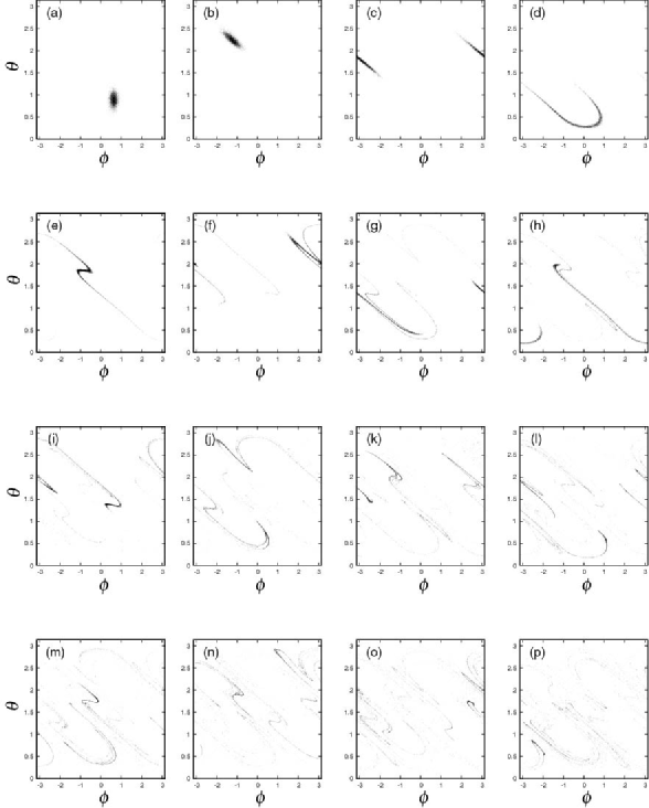
Figure 1: Classical dynamics of the distribution function with $k=3.0$. (a), (b), …, (p) corresponds to $t=0,1,\ldots,15$, respectively. The center of the initial “Gaussian” distribution function (width $\sigma=0.1$) is located at $(\theta_{0},\phi_{0})=(0.89,0.63)$.

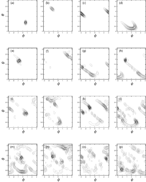
Figure 2: Quantum dynamics of the Husimi function with $j=80$ and $k=3.0$. (a), (b), …, (p) corresponds to $t=0,1,\ldots,15$, respectively. The center of the initial spin-coherent state is located at $(\theta_{0},\phi_{0})=(0.89,0.63)$.

Figures 1 and 2 show the classical dynamics of the distribution function and quantum dynamics of the Husimi function for the kicked top in a semiclassical regime ($j=80$), respectively. As is mentioned above, at the initial stage of the dynamics, the quantum-classical correspondence holds well. That is, both quantum and classical distribution functions behave very similarly. Such a precise correspondence between the distribution functions is lost as time elapses, due to quantum interference. However, even in a much longer time period, the variances of $z(t)=J_{z}(t)/j$,

$$\sigma_{\rm cl}^{2}(t) = \langle z(t)^{2}\rangle_{\rm cl}-\langle z(t)\rangle_{\rm cl}^{2},$$ (9)

$$\sigma_{\rm qu}^{2}(t) = \langle z(t)^{2}\rangle_{\rm qu}-\langle z(t)\rangle_{\rm qu}^{2},$$ (10)

have a good quantum-classical correspondence. See Fig. 3. Here $\langle\ldots\rangle_{\rm cl}$ and $\langle\ldots\rangle_{\rm qu}$ are the expectation values for the classical and the quantum systems, respectively. An explanation in terms of the classical phase-space dynamics is as follows: In the classically regular region ($k=0.5,1.0$), trajectories are trapped by tori, and the variances exhibits periodic modulations. According to the sizes (along the $J_{z}$ direction) of the trapping tori, the variances takes various values. Furthermore, the variances exhibit recurrence phenomena within a rather short time period (not shown here). On the other hand, in the classically chaotic region ($k=3.0$), both $\sigma_{\rm cl}^{2}(t)$ and $\sigma_{\rm qu}^{2}(t)$ increase rather quickly and saturate to the value $\sigma_{\rm sat}^{2}=1/3$ which is estimated by assuming a uniform distribution. In other words, the phase-space distribution functions spread uniformly all over the whole phase space, which is bounded in the case of the top.

Figure 3: Time evolution of the variances for (a) the classical and (b) quantum kicked tops. The dotted, dashed, and solid lines correspond to $k=0.5$, $1.0$, and $3.0$, respectively. The initial states of (a) and (b) are the same as in Figs. 1 and 2, respectively. Since the regular evolutions ($k=0.5,1.0$) are trapped by tori whose sizes are large in the $J_{z}$ direction, the variances takes larger value than that for the chaotic case ($k=3.0$).

III Numerical experiment of quantum kicked tops

Here we return to our motivation: How does classical chaotic dynamics affect the entanglement production of the corresponding quantum system? To investigate this issue, we employ coupled kicked tops (CKTs), which is introduced by Miller and Sarkar MS99 , as a target system of numerical experiments. The CKTs are described by the following Hamiltonian:

$$H(t)=H_{1}(t)+H_{2}(t)+H_{\epsilon}(t)$$ (11)

where

$$H_{1}(t) = \frac{k_{1}}{2j}J_{z_{1}}^{2}\sum_{n}\delta(t-n)+\frac{\pi}{2}J_{y_{1}},$$ (12)

$$H_{2}(t) = \frac{k_{2}}{2j}J_{z_{2}}^{2}\sum_{n}\delta(t-n)+\frac{\pi}{2}J_{y_{2}},$$ (13)

$$H_{\epsilon}(t) = \frac{\epsilon}{j}J_{z_{1}}J_{z_{2}}\sum_{n}\delta(t-n),$$ (14)

with $[J_{x_{l}},J_{y_{m}}]=iJ_{z_{l}}\delta_{lm}$ etc. ($l,m=1,2$). Here $k_{l}$ is the nonlinear parameter of the $l$-th top, and $\epsilon$ is the strength of the coupling between these two tops. Corresponding to the Hamiltonian, Eq. (11), we employ a Floquet operator (a one-step time-evolution operator)

$$U\equiv U_{\epsilon}U_{1}U_{2}$$ (15)

where $U_{1}=e^{-ik_{1}J_{z_{1}}^{2}/2j}e^{-i\pi J_{y_{1}}/2}$, $U_{2}=e^{-ik_{2}J_{z_{2}}^{2}/2j}e^{-i\pi J_{y_{2}}/2}$ and $U_{\epsilon}=e^{-i\epsilon J_{z_{1}}J_{z_{2}}/j}$.

Since we will consider only the case where the density operator of the total system at time $t$, $\rho(t)$, describes a pure state, we employ entropies of subsystems as measures of quantum entanglement EntanglementMeasure . More precisely, we employ von Neumann and linear entropies of the first top:

$$S_{\rm vN}(t) = -{\rm Tr}_{1}\{\rho^{(1)}(t)\ln\rho^{(1)}(t)\},$$ (16)

$$S_{\rm lin}(t) = 1-{\rm Tr}_{1}\{\rho^{(1)}(t)^{2}\},$$ (17)

where $\rho^{(1)}(t)={\rm Tr}_{2}\{\rho(t)\}$ is the reduced density operator for the first top. Note that the von Neumann entropy (or the linear entropy) of the second top takes the same value as that of the first top, when the whole system is in a pure state. To calculate $S_{\rm vN}(t)$ and $S_{\rm lin}(t)$ numerically, we use the eigenvalues $\lambda_{i}(t)$ of $\rho^{(1)}(t)$ as

$$S_{\rm vN}(t) = -\sum_{i}\lambda_{i}(t)\ln\lambda_{i}(t),$$ (18)

$$S_{\rm lin}(t) = 1-\sum_{i}\{\lambda_{i}(t)\}^{2}.$$ (19)

We numerically examine the productions of quantum entanglement, using separable states as initial states. In particular, we focus on the the system parameter dependence, i.e. $k_{1}$, $k_{2}$ and $\epsilon$ dependence, of the entanglement productions (measured by the entropies of the subsystems). For simplicity, we only show the cases where $k=k_{1}=k_{2}$. As an initial state, we employ the following pure and separable state

$$\rho(0)=|\Psi(0)\rangle\langle\Psi(0)|,$$ (20)

where $|\Psi(0)\rangle=|\theta_{1},\phi_{1}\rangle\otimes|\theta_{2},\phi_{2}\rangle$ is a direct product of spin coherent states. In studying the chaotic region, the center of the initial spin coherent state is located in the chaotic sea. Even such numerical experiments with a restricted class of initial states provides an insight about the typical behavior of chaotic CKTs, when the fraction of tori is small in phase space for the corresponding classical system (in the case of CKTs, $k>3.0$).

Figure 4 shows the time evolutions of the entropies with various values of $k$. The entropies stick to nearly zero until the “rising time”, and then they increase nearly linearly as a function of time for chaotic cases (see Figs. 4 (b),(c),(d)). Though not shown here, they saturate to finite values after the long time evolution, due to the finiteness of the dimension of the Hilbert space. In the following, we focus on the “intermediate” region where the entropies increase monotonically as a function of time. Our extensive numerical experiments conclude that, in the intermediate region, the linear entropy as well as the von Neumann entropy increases nearly linearly as a function of time, when the chaos is strong enough and the coupling is weak enough.

Figure 5 shows $\epsilon$ dependence of the linear and von Neumann entropies at $T=128$. When the coupling is weak (i.e., $\epsilon<10^{-3}$), the linear entropy obeys a perturbative behavior $S_{\rm lin}(T)\propto\epsilon^{2}$ (see Fig. 5(a)). At the same time, the time step $T=128$ belong to the region where the linear entropy increases linearly in time. In contrast to this, when $\epsilon$ is much larger than $10^{-3}$, the entropy does not belong to the perturbative region, and saturates to a finite value, which is determined by the finite size of the Hilbert space of CTKs. These observations suggests us to analyze the behavior of the linear entropy using a perturbation treatment for the interaction strength $\epsilon$. This is the subject of the next section. On the other hand, we confirmed that $S_{\rm vN}(T)\propto\epsilon^{1.8}$ when $\epsilon$ is small enough (Fig. 5 (b)). It seems that an usual perturbative treatment is difficult to explain the exponent $1.8$, so we will concentrate on the linear entropy below.

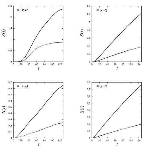
Figure 4: Time evolutions of the linear (dashed line) and von Neumann (solid line) entropies. Parameters are $\epsilon=10^{-3}$ (in an weak coupling region) and $j=80$ (in a semiclassical region). The initial state is Eq. (20) with $\theta_{1}=\theta_{2}=0.89$ and $\phi_{1}=\phi_{2}=0.63$. The center of the initial state is located in the chaotic seas for the cases of (b), (c), and (d).

Figure 5: $\epsilon$ dependence of (a) the linear and (b) von Neumann entropies at $T=128$ with $k=3.0$. The dashed lines denote $10^{6}\epsilon^{2}$ and $10^{6}\epsilon^{1.8}$ for (a) and (b), respectively. The initial state is the same as in Fig. 4.

IV Perturbative expression for the linear entropy

IV.1 Perturbation treatment

We evaluate $S_{\rm lin}(t)$, Eq. (17), the linear entropy of the first top, by using the time-dependent perturbation theory with a small parameter $\epsilon$. First, we introduce the interaction pictures, of the density matrix $\tilde{\rho}(t)=U_{0}^{\dagger}(t)\rho(t)U_{0}(t)$, and, of the operator $\hat{A}(t)=U_{0}^{\dagger}(t)AU_{0}(t)$, where $U_{0}(t)=(U_{1}\otimes U_{2})^{t}$. That is, $\hat{A}(t)$ corresponds to the “free” evolution of the operator $A$. Accordingly, the time evolution of $\tilde{\rho}(t)$ is described by the unitary mapping $\tilde{\rho}(t)=\hat{U}_{\epsilon}(t)\tilde{\rho}(t-1)\hat{U}^{\dagger}_{\epsilon}(t)$, where the expansion of $\hat{U}_{\epsilon}(t)$ by small $\epsilon$ takes the following form

$$\hat{U}_{\epsilon}(t)=1-\frac{i\epsilon}{j}\hat{V}(t)-\frac{\epsilon^{2}}{2j^{2}}\hat{V}^{2}(t)+{\cal O}(\epsilon^{3})$$ (21)

with $\hat{V}(t)=\hat{J}_{z1}(t)\hat{J}_{z2}(t)$. Hence, the unitary mapping of $\tilde{\rho}(t)$ becomes

$$\tilde{\rho}(t) = \tilde{\rho}(t-1)+\frac{i\epsilon}{j}[\tilde{\rho}(t-1),\hat{V}(t)]-\frac{\epsilon^{2}}{2j^{2}}[[\tilde{\rho}(t-1),\hat{V}(t)],\hat{V}(t)]+{\cal O}(\epsilon^{3}).$$ (22)

By induction, we have

$$\tilde{\rho}(t) = {\rho}(0)+\frac{i\epsilon}{j}\sum_{l=1}^{t}[{\rho}(0),\hat{V}(l)]$$ (23)

$$-\frac{\epsilon^{2}}{j^{2}}\sum_{l=2}^{t}\sum_{m=1}^{l-1}[[{\rho}(0),\hat{V}(l)],\hat{V}(m)]-\frac{\epsilon^{2}}{2j^{2}}\sum_{l=1}^{t}[[{\rho}(0),\hat{V}(l)],\hat{V}(l)]+{\cal O}(\epsilon^{3}).$$

By tracing out the second system, we have

$$\tilde{\rho}^{(1)}(t) = {\rho}^{(1)}(0)+\frac{i\epsilon}{j}\sum_{l=1}^{t}[{\rho}^{(1)}(0),\hat{J}_{z1}(l)]\langle\hat{J}_{z2}(l)\rangle_{2}$$ (24)

$$+\frac{\epsilon^{2}}{2j^{2}}\sum_{l=1}^{t}\left\{[\hat{J}_{z1}(l){\rho}^{(1)}(0),\hat{J}_{z1}(l)]+[\hat{J}_{z1}(l),{\rho}^{(1)}(0)\hat{J}_{z1}(l)]\right\}\langle\hat{J}^{2}_{z1}(l)\rangle_{2}$$

$$+\frac{\epsilon^{2}}{j^{2}}\sum_{l=2}^{t}\sum_{m=1}^{l-1}\left\{[\hat{J}_{z1}(l),{\rho}^{(1)}(0)\hat{J}_{z1}(m)]\langle\hat{J}_{z2}(m)\hat{J}_{z2}(l)\rangle_{2}\right.$$

$$\left.+[\hat{J}_{z1}(m){\rho}^{(1)}(0),\hat{J}_{z1}(l)]\langle\hat{J}_{z2}(l)\hat{J}_{z2}(m)\rangle_{2}\right\}+{\cal O}(\epsilon^{3})$$

where $\langle A\rangle_{2}={\rm Tr}_{2}\{\rho^{(2)}(0)A\}$ is an average for subsystem 2. Finally, we obtain a second order perturbation formula of $S_{\rm lin}(t)=S^{\rm PT}_{\rm lin}(t)+{\cal O}(\epsilon^{3})$:

$$S^{\rm PT}_{\rm lin}(t)=S_{0}\sum_{l=1}^{t}\sum_{m=1}^{t}D(l,m)$$ (25)

where $S_{0}=2\epsilon^{2}j^{2}$ and $D(l,m)$ is a correlation function of the uncoupled system. Since the interaction Hamiltonian $H_{\epsilon}(t)$, Eq. (14), is in a bilinear form, $D(l,m)$ is decomposed into a product of correlation functions of uncoupled subsystems

$$D(l,m)=C_{1}(l,m)C_{2}(l,m)$$ (26)

where

$$C_{i}(l,m)=\langle\hat{z_{i}}(l)\hat{z_{i}}(m)\rangle_{i}-\langle\hat{z_{i}}(l)\rangle\langle\hat{z_{i}}(m)\rangle_{i}\quad$$ (27)

and $\hat{z_{i}}(l)=\hat{J}_{z_{i}}(l)/j$ ($i=1,2$). In the perturbation formula, Eq. (25), $S_{0}$ is a rather trivial factor implying $S^{\rm PT}_{\rm lin}(t)\propto\epsilon^{2}$ as is observed in Fig. 5(a). The nature of the dynamics for the tops is reflected in $D(l,m)$.

Let us remark important points of our perturbation formula: (i) In common with the exact case, $S^{\rm PT}_{\rm lin}(t)$ has a symmetric form about the exchange of the first and the second tops. That is, our perturbative treatment preserves this symmetry, although we start from a perturbative treatment of the linear entropy of the first top. (ii) Our formula has a similarity with those in phenomenological descriptions of linear irreversible processes Kubo1985 , in the sense that these theories use time correlation functions to describe relaxation phenomena. This is useful both for making phenomenological arguments and for establishing a link between a phenomenological theory and a microscopic theory (cf. the linear response theory of nonequilibrium statistical mechanics Kubo1985 ); (iii) Since our approach does not take into account the effect of the recurrence, the formula (25) would have qualitatively different applicability to the classically regular and chaotic systems. For classically regular systems, our theory would break down in relatively short time period, due to the smallness of the period of the recurrence. On the other hand, for chaotic systems, we numerically confirmed that our theory works for a rather long time period.

IV.2 Comparison with numerical results

We numerically examine our formula, Eq. (25). In Fig. 6, we plot both $S_{\rm lin}(t)$ and $S^{\rm PT}_{\rm lin}(t)$ for the intermediate coupling and weak coupling cases with regular and chaotic conditions. The initial state is the direct product of the spin-coherent state as before. As shown in Fig. 5, $\epsilon=10^{-4}$ is the perturbative region, so the agreement between $S_{\rm lin}(t)$ and $S^{\rm PT}_{\rm lin}(t)$ is very good for different $k$’s up to $t\simeq 100$ (Figs. 6 (a) and (b)). Note that our perturbative expression works for such a long time to reproduce the linear increment of the entanglement productions in time. Such a correspondence degrades as $\epsilon$ gets larger, of course, as shown in Figs. 6 (c) and (d). However, as far as concerning the chaotic case $k=3.0$, our expression describes the entanglement production, at least, qualitatively.

Figure 6: Estimations of linear entropies by the perturbative formula, Eq. (25). It is compared with the exact numerical result (in dashed lines). The parameters are (a) $\epsilon=10^{-4}$ (perturbative region) with $k=1$ (regular) (b) $\epsilon=10^{-4}$ (perturbative region) with $k=3$ (chaotic), (c) $\epsilon=10^{-3}$ (intermediate region) with $k=1$ (regular), (d) $\epsilon=10^{-3}$ (intermediate region) with $k=3$ (chaotic).

V Dynamical aspects of entanglement

V.1 Harder chaos does not mean larger entanglement production

In this section, the perturbative formula, Eq. (25), is employed to answer the following question: how does the strength of chaos influence on the entanglement production rate in the strongly chaotic regions where the influences from tori are negligible.

We examine $C_{i}(l,m)$, Eq. (27), which describes the fluctuation of $z_{i}=J_{z_{i}}/j$. Since the tops are strongly chaotic, we impose several phenomenological assumptions on $C_{i}(l,m)$. Since the phase space of the kicked top is bounded, the distribution function in the phase space becomes quickly uniform in the strongly chaotic region. Hence we assume $C_{i}(l,l)\simeq\sigma_{\rm sat}^{2}$, where we ignore a short transient before the distribution function becomes uniform (see Fig. 3). The magnitude of the fluctuation $\sigma_{\rm sat}^{2}=1/3$ is determined by the assumption that the distribution function is uniform on sphere $(\theta,\phi)$. The boundedness of the phase space allows us to employ another assumption that the relaxation of $C_{i}(l,m)$ ($l\neq m$) is exponential with an exponent $\gamma_{i}$ BK83 . Furthermore, it is natural to assume that the exponent $\gamma_{i}$ becomes larger as the positive Lyapunov exponent of the corresponding classical system becomes larger. The simplest function that satisfies the assumptions above is

$$C_{i}(l,m)\simeq\sigma_{\rm sat}^{2}e^{-\gamma_{i}|l-m|}.$$ (28)

Hence $D(l,m)$, Eq. (26), becomes

$$D(l,m)\simeq D_{0}e^{-\gamma|l-m|}$$ (29)

where $D_{0}=\sigma_{\rm sat}^{4}$ and $\gamma=\gamma_{1}+\gamma_{2}$. Accordingly, Eq. (25) provides the following evaluation of the linear entropy

$$S^{\rm PT}_{\rm lin}(t)\simeq S_{0}D_{0}\left[\coth(\gamma/2)t-\frac{1-e^{-\gamma t}}{\sinh\gamma-1}\right].$$ (30)

When the relaxation time of $D(l,m)$ is much shorter than the time scale of the stationary entanglement production region, we have an entanglement production rate $\Gamma$

$$\Gamma\equiv\left.\frac{dS^{\rm PT}_{\rm lin}(t)}{dt}\right|_{t\gg 1/\gamma}\simeq\Gamma_{0}\coth(\gamma/2),$$ (31)

where $\Gamma_{0}\equiv S_{0}D_{0}$. From this relation, it is shown that $\Gamma$ decreases as $\gamma$ becomes larger, i.e. the chaos of the corresponding classical system becomes stronger. That is, the increment of the strength of chaos does not enhance the production rate of entanglement. Furthermore, in the limit $\gamma\rightarrow\infty$, $\Gamma$ quickly saturates to a finite value, $\Gamma_{0}$.

At first glance, our prediction seem to be counter-intuitive. Hence we provide an explanation of the prediction to summarize this subsection: The entanglement productions are induced by the fluctuation of the interaction Hamiltonian $H_{\epsilon}(t)$, in the interaction picture. Since the time dependence of $H_{\epsilon}(t)$ looks like very “random” in classically chaotic systems, the contribution from $H_{\epsilon}(t)$ to the linear entropy is reduced due to dynamical averaging. We note that this mechanism is similar to that of the so called motional narrowing in spin relaxation phenomena Kubo1985 ; Slichter .

V.2 Properties of the correlation function and linear entropy production rate — Saturation of the entanglement production

We test the prediction of the phenomenological argument above with numerical experiments. First, we examine the correlation function $D$, Eq. (26) (see Fig. 7). We confirmed the assumption, Eq. (29), for $D$ when the classical counterpart is chaotic ($k\geq 3.0$): The correlation function decays very quickly, althogh it is difficult to detemine the exponent $\gamma$ directly from the numerical evaluation of $D$ (see another estimation of $\gamma$ below). On the other hand, the value of $D(t,t)$ is almost independent with $k$, and approximately equal to $D_{0}=\sigma_{\rm sat}^{4}=1/9$.

Figure 7: Plot of $D^{R}(t,t-\tau)/D_{0}$ ($\equiv\Re D(t,t-\tau)/D_{0}$) as a function of $\tau$ with different $t$’s ($t=40,50,60,70$) and $k$’s. (a), (b), (c), (d) corresponds to $k=1$, $3$, $5$, $7$, respectively. The initial state is Eq. (20) with $\theta_{1}=\theta_{2}=0.89$ and $\phi_{1}=\phi_{2}=0.63$.

Second, we examine the nonlinear parameter $k$-dependence of the entanglement production rate $\Gamma$, Eq. (31). For each initial states, whose center of the spin-coherent states is placed in the chaotic sea, we obtain $\Gamma$ using the least square fitting for the time region from $t=20$ to 100, where $t$-linearity holds (Fig. 8). Hence we confirm that the increment of the strength of chaos does not enhance entanglement production rate in the perturbative regime, where $\epsilon$ is small enough. It is also confirmed that the entropy production rate $\Gamma$ saturates to $\Gamma_{0}$ for large $k$, which is also consistent with Eq. (31). At the same time, we numerically find that $\Gamma_{\rm vn}$, the entanglement production rate measured by von Neumann entropy also exhibits a saturation in the large $k$ limit. Although we do not have any analytical theory for $\Gamma_{\rm vn}$, we expect that the saturation of $\Gamma_{\rm vn}$ is explained by the similar explanation as that of the linear entropy $\Gamma$ (see Sec. V.1).

In Fig. 9, we plot $k$-dependences of two quantities: One is $\lambda_{\rm sum}\equiv\lambda_{1}+\lambda_{2}$, where $\lambda_{i}$ is the short-time (up to $t=100$) and phase-space averaged Lyapunov exponent for the initial classical distribution of $i$-th subsystem. We note that $\lambda_{\rm sum}=2\lambda_{1}$ since $k_{1}=k_{2}$. The other is the decay rate $\gamma$ of the correlation function $D$, Eq. (26). We estimate $\gamma$ from the phenomenological estimation of $\Gamma$, Eq. (31), i.e.

$$\gamma=\ln\left(\frac{\Gamma/\Gamma_{0}+1}{\Gamma/\Gamma_{0}-1}\right),$$ (32)

instead of the direct estimation from the assumption, Eq. (29). Figure 9 suggests $\gamma\simeq\lambda_{\rm sum}$. This shows an evidence that the decay rates of the correlations of tops are determined by the positive Lyapunov exponents of the classical counterparts. Thus our numerical experiments confirm the estimation, Eq. (31), and it is concluded that the entanglement production rate is not increased by the increment of the strength of chaos in the strongly chaotic region, and saturate to a finite value in the strong chaos limit.

Finally, we point out that it is natural to generalize our study on CKTs to any strongly chaotic system with bounded phase space. We note that we have already confirmed this for coupled kicked rotors SKO96 ; Lakshminarayan01 ; TAI89 with periodic boundary conditions of both position and momentum coordinates.

V.3 An extension to flow systems

In this subsection, we extend the above argument to flow systems with continuous time. Consider the case where flow systems are weakly coupled. When the initial state is a pure product state (as is the case above), the linear entropy produced in the composite system is

$$S^{\rm PT}_{\rm lin}(t)\simeq S_{0}\int_{0}^{t}d\tau\int_{0}^{t}d\tau^{\prime}D(\tau,\tau^{\prime}),$$ (33)

where $D(\tau,\tau^{\prime})$ is a correlation function determined by the form of the interaction Hamiltonian. When the subsystems are strongly chaotic with bounded phase space, we assume again

$$D(\tau,\tau^{\prime})\simeq D_{0}e^{-\gamma|\tau-\tau^{\prime}|}.$$ (34)

Substituting this into Eq. (33), we have

$$\Gamma\simeq\frac{2S_{0}D_{0}}{\gamma}(1-e^{-\gamma t})\rightarrow\frac{2S_{0}D_{0}}{\gamma}\quad(t\gg 1/\gamma).$$ (35)

Hence, if the subsystem is strongly chaotic (i.e. $\gamma\rightarrow\infty$), the entanglement production rate becomes zero. That is, strong chaos completely suppresses entanglement production! Although we have not numerically confirmed this suppression yet, the similar suppressions of quantum relaxations in strongly chaotic systems have been observed by Prosen and Žnidarič Prosen:PRE-65-036208 ; Znidaric:qph-0209145 . We will discuss this point further in Sec. VII.

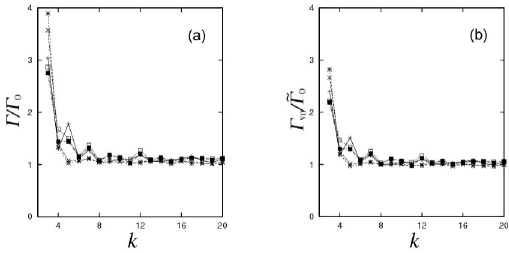
Figure 8: (a) $k$ dependence of the normalized linear entropy production rate for various initial conditions located in the chaotic sea. Note that $\Gamma$ saturates to $\Gamma_{0}$ as $k$ increases. (b) $k$ dependence of the normalized von Neumann entropy production rate $\Gamma_{\rm vN}$ for various initial conditions (the same as those of (a)) located in the chaotic sea. Note that $\Gamma_{\rm vN}$ is scaled by $\tilde{\Gamma}_{0}\equiv 2\epsilon^{1.8}j^{2}D_{0}$ instead of $\Gamma_{0}=2\epsilon^{2}j^{2}D_{0}$ (cf. Fig. 5).

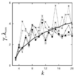
Figure 9: $k$ dependence of the correlation decay rate $\gamma$, which is determined from Eq. (32), for various initial conditions located in the chaotic sea (scattered symbols). The sum of the Lyapunov exponent $\lambda_{\rm sum}$ is also shown as a bold curve, which correspond to a single initial condition. We note that $\lambda_{\rm sum}$ depends on the initial condition only very weakly.

VI Discussion on a weakly chaotic region

In the previous section, we investigated the strongly chaotic region of the CKTs and concluded that the increment of the strength of chaos does not enhance entanglement productions, which is measured by the linear entropy of the subsystem, with the help of the perturbative formula, Eq. (25). With this in mind, we discuss the recent study by Miller and Sarkar MS99 , who investigated the weakly chaotic region (where chaotic seas and tori coexist) of the CKTs, and claimed that the increment of the strength of chaos enhances entanglement. More precisely, they numerically found that the entanglement production rate, which is measured by the von Neumann entropy, linearly depends on the sum of positive (finite-time) Lyapunov exponents of the corresponding classical CKTs, without any theoretical justification. As is well known, it is much harder to develop a theory of weakly chaotic systems (in other words, mixed phase space systems) than strongly chaotic systems. This is actually the case with the numerical result of Miller and Sarkar. To accommodate these two qualitatively different results, we employ our perturbative formula, Eq. (25), in the analysis for the weakly chaotic region ($k=3.0$, Fig. 10(a)).

In order to justify the application of our formula, Eq. (25), we confirm that the entanglement productions measured by the linear entropy, instead of the von Neumann entropy, reproduce Miller and Sarkar’s fitting. See Fig. 10(b). Furthermore, we numerically examined that the perturbative evaluation of the entanglement production rate $\Gamma$, Eq. (25), is applicable to the weakly chaotic regions, in particular the case above. Hence, in the following, we reexamine the inputs of the formula, Eq. (25), which is the correlation functions of the uncoupled systems.

We focus on our assumption, Eq. (29), for the correlation functions $D(l,m)$, Eq. (26), which is derived from Eq. (28) for strongly chaotic regions: (i) Due to the absence of tori in the corresponding classical system, the fluctuation of $z_{i}$ takes a saturated value which agrees with that of the uniform distribution in the classical phase space (i.e., $C_{i}(l,l)\simeq\sigma_{\rm sat}^{2}$); (ii) Due to the strongly chaotic dynamics, the correlation functions decays exponentially (i.e. $C_{i}(l,m)\propto e^{-\gamma_{i}|l-m|}$).

First, we examine our assumption that $\sigma_{2}$, the fluctuation of $z_{2}=J_{z}/j$, is independent of $\theta_{2}$. In the weakly chaotic region, this assumption breaks down due to the confinement of phase-space dynamics by tori. Actually, $\sigma_{2}$ becomes smaller as the “overlapping” between the initial state and tori become larger (see Fig. 11(a)). By taking account of this fact into the assumption Eq. (29) on $D(l,m)$, the decrement of $\sigma_{2}$ in tori provides a crudest explanation of the $\theta_{2}$ dependence of $\Gamma$ (denoted by $\square$ in Fig. 11(b)). That is, the decrement of the fluctuation of $z_{2}$ (denoted by $\square$ in Fig. 11 (a)) due to the influence from tori inhibits the entanglement production. See the line with $\square$ in Fig. 11 (b). However, the improved estimation denoted by $\bigcirc$ in Fig. 11 (b) still exhibits a qualitative discrepancy.

Second, to overcome this discrepancy, we improve the assumption for $D(l,m)$ as

$$D(l,m)=\sigma_{1}^{2}\sigma_{2}^{2}e^{-\gamma|l-m|}e^{i\omega(l-m)},$$ (36)

where we introduce a real-valued parameter $\omega$. This characterizes oscillations due to the regular motion of the second top. The resultant oscillation of $D(l,m)$ tends to reduce the value of $\Gamma$ in Eq. (25) (cf. Eq. (31)) :

$$\Gamma=\frac{\left({\sigma_{1}}/{\sigma_{\rm sat}}\right)^{2}\left({\sigma_{2}}/{\sigma_{\rm sat}}\right)^{2}}{1+\{\sin(\omega/2)/\sinh(\gamma/2)\}^{2}}\times\Gamma_{0}\coth(\gamma/2).$$ (37)

We determine the value of $\omega$ in Eq. (36) from the Fourier transformation of $D(l,m)$ (see Fig. 11(a)). We depict the estimation Eq. (37) (denoted by $\triangle$) also in Fig. 11 (b). We conclude that the assumption Eq. (36) provides a satisfactory improvement of the evaluation of $\Gamma$ for the weakly chaotic region that Miller and Sarkar investigated.

From our argument, it is seen that the contribution from tori also play a role for the determination of the entanglement production rate via $\sigma_{2}$ and $\omega$. Thus it is suggested that the linear dependence of $\Gamma$ with the sum of the positive Lyapunov exponents of the corresponding classical system is not intrinsic for the weakly coupling region.

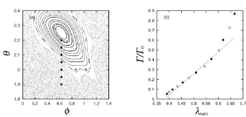
Figure 10: (a) A magnification of Poincare section of the kicked top with $k=3.0$. (b) The correlation between $\lambda_{\rm sum}$ and $\Gamma$ in a weakly chaotic region. In particular, solid circles correspond to those in (a). A linear fitting is depicted by a dashed line ($\Gamma/\Gamma_{0}=a\lambda_{\rm sum}+b$ with $a=2.2$ and $b=-0.84$). Parameters are $\epsilon=10^{-4}$ (perturbative region) and $j=80$. The center of the initial state of the first top is located at $(\phi_{1},\theta_{1})=(0.63,0.89)$, and those of the second top are depicted by solid circles in (a).

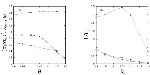
Figure 11: (a) $\theta_{2}$ dependences of $(\sigma_{2}/\sigma_{\rm sum})^{2}$ ($\square$), $\lambda_{\rm sum}$ ($\bigcirc$), and $\omega$ ($\triangle$). (b) The $\theta_{2}$ dependence of $\Gamma/\Gamma_{0}$ ($\square$). The perturbative estimations with the assumptions (29) and (36) are indicated by $\bigcirc$ and $\triangle$, respectively. Parameters and initial conditions are the same as in Fig. 10 (b). At the same time, we assume $({\sigma_{1}}/{\sigma_{\rm sat}})^{2}=1$ for the perturbative estimations.

VII Summary and outlook

We have studied how the strength of chaos affects the production rate of quantum entanglement of the coupled kicked tops (CKTs). When the coupling constant $\epsilon$ is small enough, the entanglement productions obey the perturbative formula, Eq. (25). When the classical counterpart exhibits chaotic behavior, there appears a “stationary” entanglement production regime where the entanglement production rate is well-defined. In the strongly chaotic limit, where the correlation functions of the uncoupled tops decay exponentially fast, the perturbative formula, Eq. (25), predicts that the entanglement production rate saturates to a certain value. Our numerical experiment confirmed this prediction. This is a unexpected result since the previous works show that the chaotic dynamics promotes a larger amount of quantum entanglement compared with the regular dynamics Adachi92 ; Tanaka96 ; SKO96 ; FNP98 ; Lakshminarayan01 .

Our perturbative argument of the strongly chaotic region depends only on the two points: (i) the time-correlation function of the interaction Hamiltonian decays exponentially; (ii) the phase space distributions of the corresponding classical subsystems become quickly uniform before the stationary entanglement production starts. Hence we expect that our result also holds for a wide variety of classically chaotic systems.

At the same time, we reexamined the weakly chaotic region which is recently investigated by Miller and Sarkar, who showed numerically that the entanglement production rate linearly depends on the sum of the positive linear stability exponents MS99 . Our perturbative approach provides a theoretical way to explain their result: The entanglement production rate is controlled by the combination of the decay rate, the magnitude and the oscillation frequency of the time-correlation function of the interaction Hamiltonian. It is hard to believe that these factors are generally determined only by the Lyapunov exponents. Rather, it is natural to expect that the behavior of the correlation function is strongly influenced by the existence of tori.

We point out that the investigation of dynamical production of quantum entanglement has relevance with that of quantum fidelity (measured by an overlapping integral of two states that are evolved by slightly different Hamiltonians) Fidelity ; Prosen:PRE-65-036208 . The decay of fidelity and the production of entanglement correspond to the quantum relaxations against static and dynamic disturbances, respectively. When the disturbance is small enough, the perturbative approach will describe the leading (“linear”) response. We showed that this is the case for the dynamical production of quantum entanglement. On the other hand, concerning the evaluations of quantum fidelity, Prosen et al. reported the success of a perturbative approach Prosen:PRE-65-036208 . Both works predict that the strong chaos suppresses the quantum relaxations in flow systems. Furthermore, Prosen et al. reported that their theoretical prediction on the static disturbances agrees with their numerical experiments Prosen:PRE-65-036208 . The recent studies of quantum fidelity for nonperturbative regimes NPTQF will be applicable to the studies on dynamical productions of quantum entanglement. We believe that such an effort will be fruitful to investigate “quantum chaos” in many degrees of freedom systems (see, e.g., Refs. TAI89 ; Znidaric:qph-0209145 ).

Finally, we point out a possible application of our work to the studies of realistic systems. In the investigations of chemical systems with large degrees of freedom SBPR96 including biological systems WC01 , it is important to estimate the entanglement (decoherence) rate. Most studies on this problem rely on the approaches using the master equations or the influence functional technique. However, these approaches have a serious difficulty in practical applications to chemical reaction dynamics, since the time-scale separation of the two constituents (“the system” and “the environment”) in the whole system often breaks down. In contrast to this, our approach only assumes the weakness of the coupling between the subsystems, which dynamically causes entanglement in the whole system. Hence it has an ability to cope with the breakdown of the the time-scale separation. We expect that our approach will provide a useful tool to investigate chemical reaction dynamics.

- (1) J.A. Wheeler and W.H. Zurek (editor), Quantum Theory and Measurement (Princeton University Press, Princeton, 1982).
- (2) M.A. Nielsen and I.L. Chuang, Quantum Computation and Quantum Information (Cambridge University Press, Cambridge, 2000).
- (3) W.H. Zurek and J.P. Paz, Phys. Rev. Lett. 72, 2508 (1994); G. Casati and B.V. Chirikov, ibid. 75, 350 (1995); W.H. Zurek and J.P. Paz, ibid. 75, 351 (1995).
- (4) D. Giulini, E. Joos, C. Keifer, J. Kupsch, I.-O. Stamatescu, and H.D. Zeh, Decoherence and the Appearance of a Classical World in Quantum Theory (Springer, Berlin, 1996); W.H. Zurek, Physics Today, 44, 36 (1991); Prog. Theor. Phys. 89, 281 (1993); e-print quant-ph/0105127.
- (5) M.C. Gutzwiller, Chaos in Classical and Quantum Mechanics (Springer-Verlag, New York, 1990).
- (6) S. Adachi, in Proceedings of ISKIT ’92, edited by I. Tsuda and K. Takahashi (ISIP, Iizuka, 1992), p. 76.
- (7) A. Tanaka, J. Phys. A: Math. Gen. 29, 5475 (1996).
- (8) M. Sakagami, H. Kubotani, and T. Okamura, Prog. Theor. Phys. 95, 703 (1996).
- (9) K. Furuya, M.C. Nemes, and G.Q. Pellegrino, Phys. Rev. Lett. 80, 5524 (1998).
- (10) A. Lakshminarayan, Phys. Rev. E 64, 036207 (2001).
- (11) R.M. Angelo, K. Furuya, M.C. Nemes, and G.Q. Pellegrino, Phys. Rev. E 60, 5407 (1999).
- (12) P.A. Miller and S. Sarkar, Phys. Rev. E 60, 1542 (1999).
- (13) For a brief account of this paper, see A. Tanaka, H. Fujisaki, and T. Miyadera, Phys. Rev. E 66, 045201(R) (2002).
- (14) F. Haake, M. Kuś, and R. Scharf, Z. Phys. B 65, 381 (1987); F. Haake, Quantum Signatures of Chaos, 2nd edition (Springer-Verlag, Berlin, 2000).
- (15) J.J. Sakurai, Modern Quantum Mechanics, revised edition (Benjamin/Cummings, New York, 1994).
- (16) D.A. Varshalovich, A.N. Moskalev, and V.K. Khersonskii, Quantum Theory of Angular Momentum (World Scientific, Singapore, 1988).
- (17) J.M. Radcliffe, J. Phys. A 4, 3313 (1971); F.T. Arecchi, E. Courtens, and R. Gilmore, and H. Thomas, Phys. Rev. A 6, 2211 (1972).
- (18) S.M. Barnett, and S.J.D. Phoenix, Phys. Rev. A 40, 2404 (1989).
- (19) G.P. Berman and A.R. Kolovsky, Physica D 8, 117 (1983); D.L. Shepelyansky, ibid. 8, 208 (1983).
- (20) R. Kubo, M. Toda, and N. Hashitsume, Statistical Physics II (Springer-Verlag, Berlin, 1985).
- (21) C.P. Slichter, Principles of Magnetic Resonance (Harper & Row, New York, 1963).
- (22) G. Casati, B.V. Chirikov, F.M. Izailev, and J. Ford, in Stochastic Behavior in Classical and Quantum Hamiltonian Systems, ed. by G. Casati and J. Ford, Lecture Notes in Physics, Vol. 93 (Springer, Berlin, 1979).
- (23) M. Toda, S. Adachi, and K. Ikeda, Prog. Theor. Phys. Suppl. 98, 323 (1989).
- (24) H.M. Pastawski, P.R. Levstein, and G. Usaj, Phys. Rev. Lett. 75, 4310 (1995).
- (25) T. Prosen, Phys. Rev. E 65, 036208 (2002); T. Prosen and M. Žnidarič, J. Phys. A: Math. Gen. 35, 1455 (2002).
- (26) F.M. Cucchietti, C.H. Lewenkopf, E.R. Mucciolo, H.M. Pastawski, and R.O. Vallejos, Phys. Rev. E 65, 046209 (2002) and references therein.
- (27) M. Žnidarič and T. Prosen, e-print quant-ph/0209145.
- (28) B. J. Schwartz, E. R. Bittner, O. V. Prezhdo, and P. J. Rossky, J. Chem. Phys. 104, 5942 (1996); O.V. Prezhdo and P.J. Rossky, Phys. Rev. Lett. 81, 5294 (1998); S. Okazaki, Adv. Chem. Phys. 118, 191 (2001).
- (29) A. Warshel and Z. T. Chu, J. Phys. Chem. B 105, 9857 (2001); S. Hayashi, private communication.