Path Integrals over Measurement Amplitudes:
Practical Quantum Foundations for Signal Processing and Control

Abstract

It is shown that classical control diagrams can be mapped one-to-one onto quantum path integrals over measurement amplitudes. To show the practical utility of this method, exact closed-form expressions are derived for the control dynamics and quantum noise levels of a test mass observed by a Fabry-Perot interferometer. This formalism provides an efficient yet rigorous method for analyzing complex systems such as interferometric gravity wave detectors and magnetic resonance force microscopy (MRFM) experiments. Quantum limits are conjectured for the sensitivity of interferometric observation of test mass trajectories.

I Introduction

As reviewed by Mensky Mensky (1993), the formalism of path integrals over measurement amplitudes was first suggested by Feynman Feynman (1948) and was subsequently worked out in greater detail by Mensky Mensky (1979a, b) and by Caves Caves (1986, 1987).

We show in this article that the formalism of path integrals over measurement amplitudes can provide practical quantum foundations for control theory, and we illustrate these foundations by the worked example of resonant interferometric observation of a test mass.

From a physics point of view we will work everything backwards. We will start, rather than finish, with a block diagram that describes the dynamics of a classical system that is subject to closed-loop control. We will show that such diagrams can be mapped one-to-one onto path integrals over measurement amplitudes. Then we will illustrate the physical and control-theoretic significance of each path integral term by analyzing a test mass observed by resonant optical interferometry. Finally, we will suggest that the dynamical behavior of such systems is connected to unsolved problems in quantum signal processing and cryptography.

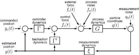
Figure 1: The control theory block diagram associated with equations (1–c), or equivalently the path integral (4–b).

II Control Theory Foundations

Engineers commonly formulate control theory in terms of block diagrams and signal-flow graphs Kuo (1991). A block diagram is conceptually similar to a Feynman diagram: it is a graphical representation of a set of equations.

Figure 1 shows a block diagram for a test mass whose position $q(t)$ is continuously measured and controlled. The control force $f_{\text{c}}(t)$ is determined from the commanded position $y_{\text{c}}(t)$ and the estimated position $y(t)$ via kernels $\Gamma$ and ${\Gamma^{\prime}}$:

$$f_{\text{c}}(t)= \int_{-\infty}^{t}\!\!\!d{t^{\prime}}\,\big{[}\Gamma(t-{t^{\prime}})(y_{\text{c}}({t^{\prime}})-y({t^{\prime}}))\big{]}$$

$$-\int_{t}^{\infty}\!\!\!d{t^{\prime}}\,{\Gamma^{\prime}}(t-{t^{\prime}})y({t^{\prime}})\,.$$ (1a)

Here by convention the feedback has been separated into a control kernel $$\Gamma {\Gamma^{\prime}}$$ that is causal and a backaction kernel that is anticausal.

Anticausal backaction kernels are a natural idiom in control theory. To see why, consider a present fluctuation in $y({t^{\prime}})$ that represents a photon detected at time ${t^{\prime}}$, having bounced off the test mass at past times $t$. It follows that the backaction kernel ${\Gamma^{\prime}}(t-{t^{\prime}})$ must be anticausal, in order to describe the past-time force exerted by those bounces. There is no implication that the backaction physics is noncausal.

To anticipate, all the other kernels of Fig. 1 are explicitly causal, and so is the path integral that we will derive for the system dynamics. The overall formalism is therefore explicitly causal, as we will discuss following (IV).

The controller kernel $\Gamma$ is the main subject of control theory; it typically serves some useful purpose like moving the test mass to a commanded position or stabilizing the system dynamics. Such kernels can be designed for optimal performance Garbini et al. (1996), and essentially any desired causal kernel can be realized by digital technology Bruland et al. (1996).

The estimated position $y(t)$ is determined from the test mass position $q(t)$ and the measurement noise $q_{\text{n}}(t)$ via the measurement kernel $\xi$:

$$y(t)=\int_{-\infty}^{t}\!\!\!d{t^{\prime}}\,\xi(t-{t^{\prime}})\big{(}q({t^{\prime}})+q_{\text{n}}({t^{\prime}})\big{)}.\\$$ (1b)

It follows that $q(t)$ cannot be observed directly, but rather must be estimated from $y(t)$; such estimation plays a central role in control theory.

Finally, the dynamical behavior of $q(t)$ is determined by the external force $f_{\text{e}}(t)$, the process noise $f_{\text{n}}(t)$, and the control force $f_{\text{c}}(t)$ via the process kernel $G$:

$$q(t)=\int_{-\infty}^{t}\!\!\!d{t^{\prime}}\,G(t-{t^{\prime}})\big{(}f_{\text{e}}({t^{\prime}})+f_{\text{n}}({t^{\prime}})+f_{\text{c}}({t^{\prime}})\big{)}.$$ (1c)

Our main statistical assumption is that $q_{\text{n}}(t)$ and $f_{\text{n}}(t)$ are stationary zero-mean random processes; we will show that path integrals naturally generate quantum noise with this property. Without loss of generality, we can further specify that $q_{\text{n}}(t)$ and $f_{\text{n}}(t)$ are statistically independent; for any given block diagram this can be arranged by “pulling” correlated noise through $G$ and suitably redefining $q_{\text{n}}(t)$ and $f_{\text{n}}(t)$.

Then the Fourier-domain solution to (1–c) is such that $\tilde{y}(\omega)$ has mean value

$$\langle\tilde{y}(\omega)\rangle=\frac{\tilde{\xi}(\omega)\tilde{G}(\omega)\,(\tilde{f}_{\text{e}}(\omega)+\tilde{\Gamma}(\omega)\tilde{y}_{\text{c}}(\omega))}{1+\tilde{\xi}(\omega)\tilde{G}(\omega)\big{(}\tilde{\Gamma}(\omega)+{\tilde{\Gamma}^{\prime}}(\omega)\big{)}}$$ (2a)

and spectral density

$$S_{y}(\omega) =\frac{|\tilde{\xi}(\omega)|^{2}\,\big{(}S_{q}(\omega)+|\tilde{G}(\omega)|^{2}S_{f}(\omega)\big{)}}{\big{|}1+\tilde{\xi}(\omega)\tilde{G}(\omega)\big{(}\tilde{\Gamma}(\omega)+{\tilde{\Gamma}^{\prime}}(\omega)\big{)}\big{|}^{2}}.$$ (2b)

The form of this result reflects our convention that the measurement noise $q_{\text{n}}(t)$ and the process noise $f_{\text{n}}(t)$ are uncorrelated. Here our notation and normalization convention for Fourier transforms and spectral densities is

$$S_{f}(\omega) \overset{\scriptscriptstyle\text{def}}{=}\int_{-\infty}^{\infty}d\tau\,\langle f(0)f(\tau)\rangle e^{-i\omega\tau},$$ (3a)

$$\tilde{f}(\omega) \overset{\scriptscriptstyle\text{def}}{=}\int_{-\infty}^{\infty}d\tau\,f(\tau)e^{-i\omega\tau},$$ (3b)

$$\tilde{\psi}(\omega,{\omega^{\prime}}) \overset{\scriptscriptstyle\text{def}}{=}\int_{-\infty}^{\infty}d\tau d{\tau^{\prime}}\,\psi(\tau,\tau^{\prime})e^{-i(\omega\tau+{\omega^{\prime}}{\tau^{\prime}})},$$ (3c)

with $\langle\ldots\rangle$ designating an ensemble average. Thus our spectral densities are “two-sided.” We regard the kernels of (1–c) as defined for all times $\tau$ with $\Gamma(\tau)=\xi(\tau)=G(\tau)=0$ for $\tau<0$ and ${\Gamma^{\prime}}(\tau)=0$ for $\tau>0$.

As a mathematical point, the functions $f_{\text{n}}(t)$ and $q_{\text{n}}(t)$ in the block diagram of Fig. 1 do not appear as independent functions in (2a–b). Neither will these functions appear as independent variables in our path integrals—not even as dummy variables of integration—nor will they appear in any subsequent part of our formalism. Their sole role is as mnemonic aids: they remind us to include $S_{f}$ and $S_{q}$ in (2b).

Since $f_{\text{n}}(t)$ and $q_{\text{n}}(t)$ do not appear in our formalism as indendent functions, we have no mathematical or physical basis for assigning independent meanings to them. We can only speak of them in terms of a unitary equivalent noise having, e.g., spectral density $S_{f}(\omega)+|\tilde{G}(\omega)|^{-2}S_{q}(\omega)$ at the $G$ block input, per Fig. 1. Again anticipating future results, our sole motivation for maintaining $S_{f}(\omega)$ and $S_{q}(\omega)$ as separate densities is to express the noise reciprocity relation (19) in a device-independent form.

This unitary point of view is consonant with information theory, since in light of the above discussion it is not possible—even in principle—to infer independent values for $f_{\text{n}}(t)$ and $q_{\text{n}}(t)$ from the measured quantity $y(t)$. Furthermore, maintaining a unitary point of view will forestall conceptual difficulties in Section VI, where we compare path integral results with analyses of shot noise and radiation-pressure noise in the literature.

III Path Integral Representations
of Control Theory

Now we seek a path integral that reproduces ((2a–b)). We approach this as a purely mathematical exercise whose sole requirements are tractability and generality. Adopting the path integral notation of Brown Brown (1992), we consider functionals of the form

$$P(y(t) |f_{\text{e}}(t),y_{\text{c}}(t))=$$

$$\left|\int[dq]\exp\big{[}\mathcal{A}(q(t),y(t),f_{\text{e}}(t),y_{\text{c}}(t))\big{]}\right|^{2}.$$ (4a)

Here $$P(y(t)|f_{\text{e}}(t),y_{\text{c}}(t))$$ is a Gaussian probability functional whose mean and variance must reproduce (2a–b).

Table 1: Table of functional densities that appear in (4). See Table 2 for the connection between the kernels $\{\Gamma,{\Gamma^{\prime}},\theta,\psi,\xi\}$ of these densities and the system dynamics specified by Eqs. (2a–b).

Lagrangian test mass action
$\mathcal{L}(q(t))$$\,=\,$	$\displaystyle\frac{{\dot{q}}^{2}(t)}{2m}-\frac{1}{2}m\omega_{0}^{2}q^{2}(t)$ $\ \Leftrightarrow\$	$\left\{\text{\parbox{224.03743pt}{\raggedright The Lagrangian of a test particle of mass $m$ with (optional) spring constant $m\omega_{0}^{2}$.\@add@raggedright}}\right.$
External force and control functionals
$\mathcal{H}_{\text{f}}(q(t),f_{\text{e}}(t))$$\,=\,$	$\displaystyle-q(t)f_{\text{e}}(t)$ $\ \Leftrightarrow\$	$\left\{\text{\parbox{224.03743pt}{\raggedright Generates the dynamical effects of the external \\ force $f_{\text{e}}(t)$.\@add@raggedright}}\right.$
$\mathcal{H}_{\Gamma}(q(t),y(t),y_{\text{c}}(t))$$\,=\,$	$\displaystyle-q(t)\!\!\int_{-\infty}^{\infty}\!\!\!d{t^{\prime}}\,\Gamma(t-{t^{\prime}})(y_{\text{c}}({t^{\prime}})-y({t^{\prime}}))$ $\ \Leftrightarrow\$	$\left\{\text{\parbox{224.03743pt}{\raggedright Generates the control force appropriate to the commanded position $y_{\text{c}}(t)$.\@add@raggedright}}\right.$
Measurement functionals
$\mathcal{M}_{{\Gamma^{\prime}}}(q(t),y(t))$$\,=\,$	$\displaystyle+q(t)\!\!\int_{-\infty}^{\infty}\!\!\!d{t^{\prime}}\,{\Gamma^{\prime}}(t-{t^{\prime}})y({t^{\prime}})$ $\ \Leftrightarrow\$	$\left\{\text{\parbox{224.03743pt}{\raggedright Generates a fluctuating backaction force that is deterministically correlated with fluctuations in $y(t)$.\@add@raggedright}}\right.$
$\mathcal{M}_{\theta}(q(t),b(t))$$\,=\,$	$\displaystyle-b(t)\!\!\int_{-\infty}^{\infty}\!\!\!d{t^{\prime}}\,\theta(t-{t^{\prime}})q({t^{\prime}})$ $\ \Leftrightarrow\$	$\left\{\text{\parbox{224.03743pt}{\raggedright Generates a backaction force parameterized by the deterministic function $b(t)$.\@add@raggedright}}\right.$
$\mathcal{M}_{\psi}(q(t),r(t))$$\,=\,$	$\displaystyle+\frac{1}{2}\int_{-\infty}^{\infty}\!\!\!d{t^{\prime}}\,dt^{\prime\prime}\,\psi(t-t^{\prime},t-t^{\prime\prime})q({t^{\prime}})q(t^{\prime\prime})$ $\ \Leftrightarrow\$	$\left\{\text{\parbox{224.03743pt}{\raggedright Generates a frequency-dependent backaction \\ spring constant.\@add@raggedright}}\right.$
$\hskip 10.00002pt\mathcal{M}_{\xi}(q(t),y(t),r(t))$$\,=\,$	$\displaystyle-\frac{\hbar}{4\gamma^{2}}\Big{(}y(t)-\!\!\int_{-\infty}^{\infty}\!\!\!d{t^{\prime}}\,\xi(t-{t^{\prime}})q({t^{\prime}})\Big{)}^{2}$ $\ \Leftrightarrow\$	$\left\{\text{\parbox{224.03743pt}{\raggedright Correlates the measured value $y(t)$ with the test \\ mass position $q(t)$.\@add@raggedright}}\right.$

For $P$ to be of the required Gaussian form, the action functional $\mathcal{A}$ must be biquadratic in $q(t)$ and $y(t)$ and bilinear in $f_{\text{e}}(t)$ and $y_{\text{c}}(t)$. Note that $q(t)$ appears only as a dummy variable of integration that is not yet identified as the test mass trajectory of Fig. 1. Adopting a conventional form that facilitates subsequent connection to control theory, the most general functional $\mathcal{A}$ that reproduces (2a–b) can be written as

$$\mathcal{A} =\int_{-\infty}^{\infty}\frac{dt}{i\hbar}\,\big{[}\,-\mathcal{L}$$ Lagrangian action

$$\quad+\mathcal{H}_{\text{f}}+\mathcal{H}_{\Gamma}$$ external force and control

$$\quad+\mathcal{M}_{{\Gamma^{\prime}}}+\mathcal{M}_{\theta}+\mathcal{M}_{\psi}$$ backaction effects

$$\quad+i\mathcal{M}_{\xi}\,\big{]}$$ measurement amplitude (4b)

where $\{\mathcal{L},\mathcal{H}_{\text{f}},\mathcal{H}_{\Gamma},\mathcal{M}_{{\Gamma^{\prime}}},\mathcal{M}_{\theta},\mathcal{M}_{\psi},\mathcal{M}_{\xi}\}$ are real-valued functionals that are given explicitly in Table 1 in terms of measurement kernels $\{{\Gamma^{\prime}},\Gamma,\theta,\psi,\xi\}$. Carrying through the path integral by methods that are essentially algebraic Brown (1992), we connect the kernels of (4b) to the control dynamics of (2a–b), as summarized in Table 2.

This completes our goal of establishing a path integral representation of the control diagram of Fig. 1.

Table 2: The connection between the measurement kernels $\{\psi,\theta,\xi\}$ of Table 1 and the system dynamics and noise specified by Eqs. (2a–b) and Fig. 1.

Backaction dynamical effects
$\tilde{G}^{-1}(\omega)$$\,=\,$	$m(\omega_{0}^{2}-\omega^{2})+\tilde{\psi}(\omega,-\omega)$ $\ \Leftrightarrow\$	$\left\{\text{\parbox{79.49744pt}{\raggedright dynamical kernel.\@add@raggedright}}\right.$
$\tilde{f}_{\text{e}}(\omega)$$\,=\,$	$\tilde{b}(\omega)\tilde{\theta}(-\omega)$ $\ \Leftrightarrow\$	$\left\{\text{\parbox{79.49744pt}{\raggedright backaction force.\@add@raggedright}}\right.$
Measurement noise PSDs
$S_{q}(\omega)$$\,=\,$	$\displaystyle\frac{\gamma^{2}}{|\xi(\omega)|^{2}}$ $\ \Leftrightarrow\$	$\left\{\text{\parbox{79.49744pt}{\raggedright measurement noise.\@add@raggedright}}\right.$
$S_{f}(\omega)$$\,=\,$	$\displaystyle\frac{\hbar^{2}}{4S_{q}(\omega)}$ $\ \Leftrightarrow\$	$\left\{\text{\parbox{79.49744pt}{\raggedright force noise.\@add@raggedright}}\right.$

IV The Measurement Amplitude For Optical Interferometry

To show what is gained by attacking the problem in this systematic way, we now calculate the measurement amplitude kernels $\{{\Gamma^{\prime}},\Gamma,\theta,\psi,\xi\}$ for a resonant optical interferometer. Then we systematically read off the system dynamics and quantum noise from Tables 1 and 2 and Eqs. (2a–b).

To carry through this calculation—and indeed to carry through any path integral/measurement amplitude calculation—it suffices to specify the classical optical scattering amplitude and the photon detection statistics. From classical physics we know that for a general single-port optical device the outgoing amplitude $a_{\text{out}}$ at time $t$ is causally conditioned upon the past history of the internal coordinate $q(t)$ as follows:

$$a_{\text{out}}(t|q(t))=a_{\text{in}}e^{i\zeta}\,\bigg{(}1+\int_{-\infty}^{t}\!\!d{t^{\prime}}\,\alpha(t-{t^{\prime}})q({t^{\prime}})$$

$$\qquad+\int_{-\infty}^{t}\!\!d{t^{\prime}}\int_{-\infty}^{t}\!\!d{t^{\prime\prime}}\,\beta(t-{t^{\prime}},t-{t^{\prime\prime}})q({t^{\prime}})q({t^{\prime\prime}})\bigg{)}.$$ (5)

Here $a_{\text{in}}$ is the input light amplitude (assumed constant), $\alpha$ and $\beta$ are scattering kernels, and $e^{i\zeta}$ is an overall phase. Perturbations of order $q^{3}$ and higher are neglected, and by convention we normalize $a_{\text{in}}$ such that the photon input rate is $r_{\text{in}}=|a_{\text{in}}|^{2}$. Causal boundary conditions are imposed. Then the mean rate $\langle r(t)\rangle$ at which photons are detected at time $t$ is a functional of the past trajectory $q(t)$: $\langle r(t)\rangle=|a_{\text{out}}(t|q(t))|^{2}$.

Now we are ready for the key element of our formalism. We introduce as an ansatz the following fundamental relation between the quantum measurement action of (4–b) and the classical scattering amplitude (IV):

$$\exp\left[\frac{\mathcal{M}(r(t),q(t))}{i\hbar}\right] =\left[\frac{a_{\text{out}}(t|q(t))}{|a_{\text{out}}(t|q(t))|}\right]^{r(t)}$$

$$\times\exp\left[\frac{-(r(t)-|a_{\text{out}}(t|q(t))|^{2})^{2}}{4\alpha_{\text{s}}|a_{\text{out}}(t|q(t))|^{2}}\right].$$ (6)

Here $\mathcal{M}(r(t),q(t))\overset{\scriptscriptstyle\text{def}}{=}\mathcal{M}_{{\Gamma^{\prime}}}+\mathcal{M}_{\theta}+\mathcal{M}_{\psi}+i\mathcal{M}_{\xi}$ is the measurement action that appears in (4–b).

We will present no field-theoretic justification for this ansatz, and in Section VIII we will present reasons for thinking that a rigorous field-theoretic justification would involve deep quantum-informatic issues. Instead, our limited goal in this article will be to show that the ansatz reproduces, within a path integral formalism, known classical and quantum physics.

From the ansatz we immediately obtain rules for translating the optical kernels $\alpha$ and $\beta$ into the measurement amplitude $\mathcal{M}$ of (IV). No physical insight is employed; instead we impose the purely algebraic requirement that the rules convert (IV) into an identity (up to $\mathcal{O}(q^{2})$ in the path integral functional). The rules are summarized in Table 3. Because the optical kernels $\alpha$ and $\beta$ satisfy causal boundary conditions, the measurement amplitude (IV) and the resulting path integral (4) are explicitly causal as promised in the discussion following (1).

Table 3: Rules connecting the photon sideband amplitudes $\{\alpha,\beta\}$ to the measurement amplitudes $\{\psi,\theta,\xi,\Gamma\}$ of Tables 1 and 2 for the interferometer configuration of Fig. 2

Fields and variables
$\tilde{y}(\omega)$$\,=\,$	$\displaystyle\tilde{r}(\omega)-2\pi r_{\text{in}}\delta(\omega)$ $\ \Leftrightarrow\$	$\left\{\text{\parbox{86.72377pt}{\raggedright photon flux\\ fluctuations.\@add@raggedright}}\right.$
$\tilde{b}(\omega)$$\,=\,$	$2\pi r_{\text{in}}\delta(\omega)$ $\ \Leftrightarrow\$	$\left\{\text{\parbox{86.72377pt}{\raggedright light pressure.\@add@raggedright}}\right.$
$\gamma^{2}$$\,=\,$	$\displaystyle\alpha_{\text{s}}r_{\text{in}}$ $\ \Leftrightarrow\$	$\left\{\text{\parbox{86.72377pt}{\raggedright Sets the flux spectral density $S_{r}=\alpha_{\text{s}}r_{\text{in}}$.\@add@raggedright}}\right.$
Measurement kernels
${\tilde{\Gamma}^{\prime}}(\omega)$$\,=\,$	$\displaystyle-\frac{\hbar}{2i}\big{[}\tilde{\alpha}(-\omega)-\tilde{\alpha}^{\star}(\omega)\big{]}$ $\ \Leftrightarrow\$	$\left\{\text{\parbox{86.72377pt}{\raggedright backaction control kernel.\@add@raggedright}}\right.$
$\tilde{\theta}(\omega)$$\,=\,$	$-{\tilde{\Gamma}^{\prime}}(-\omega)$ $\ \Leftrightarrow\$	$\left\{\text{\parbox{86.72377pt}{\raggedright couples light pressure to the test mass.\@add@raggedright}}\right.$
$\tilde{\psi}(\omega)$$\,=\,$	$-\hbar r_{\text{in}}\,$ $\text{Im}\big{[}\,2\tilde{\beta}(\omega,-\omega)$ $-{\tilde{\alpha}}(\omega){\tilde{\alpha}}(-\omega)\big{]}$ $\ \Leftrightarrow\$	$\left\{\text{\parbox{86.72377pt}{\raggedright frequency-dependent spring constant.\@add@raggedright}}\right.$
$\tilde{\xi}(\omega)$$\,=\,$	$\displaystyle r_{\text{in}}\big{[}{\tilde{\alpha}}(\omega)+{\tilde{\alpha}}^{\star}(-\omega)\big{]}$ $\ \Leftrightarrow\$	$\left\{\text{\parbox{86.72377pt}{\raggedright measurement kernel.\@add@raggedright}}\right.$

Non-rigorously, the ansatz can be derived by constructing a numerical wave function simulation along the lines given by Gardiner and Zoller Gardiner and Zoller (2000), with each photon detected separately and accounted numerically. Such simulations become exponentially slower as the number of photons and the multiple reflections of each photon are increased; this illustrates the well-known nonpolynomial difficulty of quantum simulation in general. Coding such simulations with a view to making them numerically efficient leads naturally to a path integral formalism. This is the path the author followed to the results of this article.

The ansatz embodies two key physical principles, which are both well satisfied in optical interferometry. First, individual photons are assumed to be detected discretely, such that the decoherence associated with each detection event procedes to completion within a very short time compared to all other dynamical time scales of the system. Under these circumstances a well-defined phase can be associated with photon detection. The interference of these phases can be readily observed, which is of course the reason such measurements are called “interferometric”. The ansatz functional $\left(a_{\text{out}}/|a_{\text{out}}|\right)^{r(t)}$ accumulates the test mass phase from repeated photon detections; this phase creates the quantum backaction.

Second, it is assumed that large numbers of photons are detected, in which case the detection statistics can reasonably be described by a counting formula of the usual Gaussian form (the lower right-hand term in (IV)), such that the photon flux spectral density is $S_{r}=\alpha_{\text{s}}r_{\text{in}}$, with due allowance for photon number squeezing as parametrized by $\alpha_{\text{s}}$. The physical role of the Gaussian term is to restrict the domain of path integration, conditioned upon the flux measurement $r(t)$, in precisely the manner envisioned by Feynman, Mensky, and Caves.

V A Worked Example:
Single-Port Fabry-Perot Interferomtry

To make the path integral/measurement amplitude formalism come alive we will apply it to an engineering analysis of the Fabry-Perot cavity shown in Fig. 2. This is a single-arm interferometer with single-port detection; it is not intended to represent a realistic gravity wave detector. However, even this simple design exhibits complex dynamical and noise phenomena; our goal is to show how to use path integral methods in analyzing this behavior.

Many of the results that we will obtain by path integration have also recently been obtained by operator methods in the literature on gravity wave detection; this literature is reviewed in Section VI. We will find no serious conflict between operator methods and the path integral/measurement amplitude formalism.

In applying the path integral formalism, our sole computational job is to calculate the optical kernels $\tilde{\alpha}(\omega)$ and $\tilde{\beta}(\omega,-\omega)$ of (IV) for the Fabry-Perot cavity of Fig. 2; the rest is substitution into the rules of Tables 2 and 3.

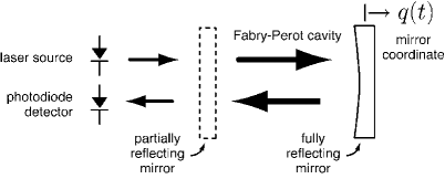
Figure 2: A Fabry-Perot cavity, with the end mirror serving as a test mass with coordinate $q(t)$.

The input light is right-going, as shown in Fig. 2, and our phase convention is that it has space-time dependence $a(x,t)=a_{\text{in}}e^{ikx-\omega_{0}t}$, where the wave number $k$ and the optical carrier freqency $\omega_{0}$ are positive quantities. This accords with the quantum mechanics phase convention that a right-going quantum carrying momentum $\hbar k$ has a spatial wave function $\propto e^{ikx}$. With this convention, positive mirror displacements $q(t)$ correspond to longer cavity lengths, as shown in Fig. 2, and positive forces act to push the mirrors apart.

This same phase convention, when conjoined with the Fourier convention (3b), prescribes that optical sidebands at a frequency $\omega_{\text{m}}$ have a Doppler-shifted time-dependence $e^{-i\omega_{0}t+i\omega_{\text{m}}t}$. Positive-frequency sidebands ($\omega_{\text{m}}>0$) are therefore associated with redshifted optical quanta. This unintuitive convention will be important later on when we check energy conservation.

Inspection of Table 3 shows that the dynamical and noise behavior of the system is completely determined by the Fabry-Perot sideband amplitude $\tilde{\alpha}(\omega)$ and carrier amplitude $\tilde{\beta}(\omega,-\omega)$. A straightforward perturbative calculation yields for the sideband

$$\tilde{\alpha}(\omega)=\frac{2ike^{i(3\omega\tau-2\phi)}\sin^{2}\rho}{(e^{2i(\omega\tau-\phi)}-\cos\rho)(1-e^{-2i\phi}\cos\rho)},$$ (7a)

and for the carrier

$$\frac{\tilde{\beta}(\omega,-\omega)}{\tilde{\alpha}(\omega)\tilde{\alpha}(-\omega)}=\frac{\sin^{2}\rho+2i\sin(2\phi)\cos\rho}{2\sin^{2}\rho}.$$ (7b)

Here the power reflectivity of the input mirror is by definition $\cos^{2}\rho$, and the one-way optical phase length $\phi$ of the cavity is $\phi=kL+\pi$, with $L$ the cavity length. The extra $\pi$ in the definition of $\phi$ is conventional; it ensures that tuning to $\phi=0\pmod{2\pi}$ yields maximal intracavity optical power. For fixed $\phi$, and therefore fixed optical power, we can maximize the sideband amplitude by tuning the mirror modulation frequency $\omega$ to $\omega\tau=\phi\pmod{2\pi}$; this is physically equivalent to tuning the sideband on-resonance.

The same perturbative calculation yields for the phase $e^{i\zeta}$ of the output light

$$e^{i\zeta}=\frac{e^{-2i\phi}\cos\rho-1}{\cos\rho-e^{-2i\phi}},$$ (8)

and it is easy to check that $|e^{i\zeta}|=1$. It is also useful to know the cavity power gain $\mathcal{G}(\phi)$:

$$\mathcal{G}(\phi)\overset{\scriptscriptstyle\text{def}}{=}\frac{\text{cavity power}}{\text{input power}}=\left|\frac{\sin\rho}{\cos\rho-e^{-2i\phi}}\right|^{2}.$$ (9)

$\mathcal{G}(\phi)$ is a period-$\pi$ function of $\phi$, peaked about $\phi\sim 0$, and having half-width-half-maximum $\phi_{\mathcal{F}}$

$$\phi_{\mathcal{F}}=\frac{1}{2}\,\sqrt{\cos\rho+\cos^{-1}\rho-2}.$$ (10)

By construction, $\phi_{\mathcal{F}}$ is the extra phase length required to reduce the on-resonance cavity power by 1/2. Conventionally $\mathcal{F}\equiv\pi/(2\phi_{\mathcal{F}})$ is called the finesse of the cavity, and for high-finesse cavities the on-resonance intracavity power gain is $\mathcal{G}(0)\simeq 2\mathcal{F}/\pi=\phi_{\mathcal{F}}^{-1}$. We will always specify changes in cavity length as multiples of $\phi_{\mathcal{F}}$.

Now we are ready to specify an interferometer design. We choose length scales and power levels that are characteristic of recent proposals for advanced gravity-wave detectors Fritschel et al. (2002):

cavity length:	$L$	$=4\ \text{km}$
detected power:	$P_{\text{out}}$	$=180\ \text{W}$
on-resonance power:	$P_{\text{max}}$	$=830\ \text{kW}$
light wavelength:	$\lambda$	$=1064\ \text{nm}$
test mass:	$m$	$=40\ \text{kg}$

This is a high-finesse cavity, with $\mathcal{F}\simeq 7240$, corresponding to a mirror power reflectivity $\cos^{2}\rho\simeq 0.99913$.

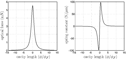
Figure 3: Static force and spring constant generated by the intra-cavity light. Here $\phi\overset{\scriptscriptstyle\text{def}}{=}kL+\pi$, with $L$ the cavity length and $k$ the optical wavenumber, and $\phi_{\mathcal{F}}$ is defined in (10).

We begin by considering the static behavior of the system. The path integral prediction for the light force ${f}_{\text{e}}(t)$ on the mirror can be read off from Tables 2 and  3:

$${f}_{\text{e}}(t) \overset{\scriptscriptstyle\text{def}}{=}{\textstyle\int_{-\infty}^{\infty}\!\!\frac{d\omega}{2\pi}}\,e^{i\omega t}\tilde{f}_{\text{e}}(\omega)$$ by definition

$$={\textstyle\int_{-\infty}^{\infty}\!\!\frac{d\omega}{2\pi}}\,\tilde{b}(\omega)\tilde{\theta}(-\omega)$$ by Table 2

$$={\textstyle\int_{-\infty}^{\infty}\!\!\frac{d\omega}{2\pi}}\,(-2\pi r_{\text{in}})\delta(\omega){\tilde{\Gamma}^{\prime}}(\omega)$$ by Table 3

$$=-r_{\text{in}}{\tilde{\Gamma}^{\prime}}(0)$$ by evaluation

$$=r_{\text{in}}\,\frac{\hbar}{2i}\big{[}\tilde{\alpha}(0)-\tilde{\alpha}^{\star}(0)\big{]}$$ by Table 3

By explicit calculation we check that this accords with the standard expression for light pressure:

$${f}_{\text{e}}(t)\overset{\hskip 1.72218pt\raisebox{-1.07639pt}[0.0pt][0.0pt]{\includegraphics[width=4.73611pt]{PIMA_checkCharacter.epsf}}}{=}2\hbar kr_{\text{in}}\mathcal{G}(\phi).$$ (11)

Here $2\hbar k$ is the momentum transferred to the mirror by the reflection of a single photon and $r_{\text{in}}\mathcal{G}(\phi)$ is the flux of photons incident on the mirror.

Similarly, from Table 2 we see that the zero-frequency spring constant exerted by the light is $k_{\text{spring}}(\phi)\overset{\scriptscriptstyle\text{def}}{=}\lim_{\omega\to 0}\tilde{\psi}(\omega,-\omega)$, and by explicit calculation we check that this accords with the spring constant predicted from the cavity gain $\mathcal{G}(\phi)$:

$$k_{\text{spring}}(\phi)\overset{\hskip 1.72218pt\raisebox{-1.07639pt}[0.0pt][0.0pt]{\includegraphics[width=4.73611pt]{PIMA_checkCharacter.epsf}}}{=}-2\hbar k^{2}r_{\text{in}}\frac{\partial\mathcal{G}(\phi)}{\partial\phi}.$$ (12)

As a final check on the static physics, it is straightforward to show that the large $\mathcal{F}$ limit of $k_{\text{spring}}(\phi)$ precisely accords with the Fabry-Perot spring constant calculated by Braginsky, Khalili, and Volikov Braginsky et al. (2001a) from classical physics. We thus confirm that the path integral/measurement amplitude method accurately reproduces known results relating to static optical forces and springs in resonant cavities.

In subsequent calculations we will not show all the steps, but our results are always obtained by a similarly direct application of the measurement amplitude rules given in Tables 2–3. These rules are readily processed by symbolic programs; this reduces the incidence of algebraic error. Analytic continuation is straightforward because the kernels are given in closed form; we will see that this simplifies stability analysis.

Now we turn our attention to the practical challenge of tuning the interferometer for dynamical stability and good noise performance. The static optical force and spring constant are shown in Fig. 3. The optical forces are weak—a few millinewtons at most—but the spring constant can approach 100 N/$\mu$m, which is extraordinarily stiff. For an optical beam of nominal diameter 20 cm and length 4 km the stiffness is equivalent to a modulus $\sim 12.3$ TPa, which is twelve times stiffer than an equivalent bar of diamond.

This illustrates that light itself can serve as a structural material, as was first recognized and explored for design purposes by Braginsky, Gorodetsky and Khalili Braginsky et al. (1997); Braginsky and Khalili (1999); Khalili (2001) and subsequently by Buonanno and Chen Buonanno and Chen (2001a, 2002a, 2002b).

By inspection of Fig. 3 we see that static stability is possible if and only if the interferometer is tuned “long” (i.e., cavity phase length $\phi>0$), and we henceforth confine our attention to this range. In practice, tuning is achieved by applying a few mN of force to the mirror to press it against the optical spring; the magnitude of the static force determines the equilibrium cavity length and therefore the optical tuning.

Static stability does not guarantee dynamic stability, and on physical grounds we expect Fabry-Perot cavities to be dynamically unstable. We reason as follows: if we push the mirror against the optical spring, the spring will push back, but only after a time lag while the intracavity intensity builds up. By oscillating the mirror, we can continuously extract energy from the system.

Physically, the possibility of energy extraction indicates the presence of dynamical instability. We will now prove that such instabilities exist—for all cavity tunings—by calculating the transfer function of the system in closed analytic form.

We begin by noting that the time-averaged flux of output photons from any linear lossless optical device must equal the flux of input photons. It is easy to check that the Fabry-Perot amplitudes (7a–b) satisfy this constraint, which requires that $\{\alpha,\beta\}$ satisfy

$$|\tilde{\alpha}(\omega)|^{2}+|\tilde{\alpha}(-\omega)|^{2} \overset{\hskip 1.72218pt\raisebox{-1.07639pt}[0.0pt][0.0pt]{\includegraphics[width=4.73611pt]{PIMA_checkCharacter.epsf}}}{=}-2*\text{Re}\big{[}\tilde{\beta}(\omega,-\omega)\big{]},$$ (13)

[sideband photon flux] $$=\text{[decreased carrier flux]}.$$

Physically, photons that disappear from the carrier must reappear in the sidebands.

This does not guarantee energy conservation, since the outgoing sideband photons are Doppler shifted per the discussion preceding (7a–b). To check energy conservation we apply an external force $f_{\text{e}}(t)$ to the mirror, such that the mirror is driven at an amplitude $q(t)=q_{0}\cos(\omega_{\text{m}}t)$. Then mechanical energy is supplied to the mirror at a rate given by (2a) as

$$\langle f_{\text{e}}(t){\dot{q}}(t)\rangle_{t}=i\omega_{\text{m}}\frac{q_{0}^{2}}{4}\, \left[{\tilde{\Gamma}^{\prime}}(-\omega_{\text{m}})\tilde{\xi}(-\omega_{\text{m}})\right.$$

$$\left.\qquad-\,{\tilde{\Gamma}^{\prime}}(\omega_{\text{m}})\tilde{\xi}(\omega_{\text{m}})\right]$$ (14)

with $\langle\ldots\rangle_{t}$ denoting a time average. After substitution from Tables 2 and 3 this is

$$\langle f_{\text{e}}(t){\dot{q}}(t)\rangle_{t}\overset{\hskip 1.72218pt\raisebox{-1.07639pt}[0.0pt][0.0pt]{\includegraphics[width=4.73611pt]{PIMA_checkCharacter.epsf}}}{=}\hbar\omega_{\text{m}}r_{\text{in}}\frac{q_{0}^{2}}{4}\left[|\tilde{\alpha}(-\omega_{\text{m}})|^{2}-|\tilde{\alpha}(\omega_{\text{m}})|^{2}\right].$$ (15)

Taking into account the Doppler sign convention discussed at the start of this section, we recognize this as precisely the excess optical power emitted in the sidebands. Thus the optomechanical instability is energetically driven by Doppler shifts in the sidebands, such that energy is explicitly conserved overall.

Now we analyze the instability in detail. From (2a), the transfer function $\tilde{T}(\omega)$ for the cavity is

$$\tilde{T}(\omega)\overset{\scriptscriptstyle\text{def}}{=}\hbar kc\,\frac{\tilde{y}(\omega)}{\tilde{f}_{\text{e}}(\omega)}=\hbar kc\,\frac{\tilde{\xi}(\omega)\tilde{G}(\omega)}{1+\tilde{\xi}(\omega)\tilde{G}(\omega){\tilde{\Gamma}^{\prime}}(\omega)}$$ (16)

where the factor $\hbar kc$ normalizes $\tilde{T}(\omega)$ to units of watts of detected optical power per newton of applied force.

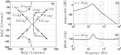
Figure 4: Dynamical behavior of the test mass. (a) Poles of the transfer function $\tilde{T}(\omega)$ as the cavity tuning is varied over $0<\phi<\infty$. The specific tunings $\phi/\phi_{\mathcal{F}}\in\{0.01,0.1,1,10\}$ are marked with a ‘    ’. A fixed zero at $s=0$ is marked with a ‘${\bm{\circ}}$’. (b-c) A Bode plot of $\tilde{T}(\omega)$ evaluated for the particular cavity tuning $\phi=10\,\phi_{\mathcal{F}}$. The magnitude axis is $20\,\log_{10}|\tilde{T}(2\pi f)\ \text{N}/\mu\text{W}|$.

In control theory—where Laplace transforms are more common than Fourier transforms—it is standard practice to plot the dominant poles and zeros of the transfer function in the complex $s$-plane, with $s\overset{\scriptscriptstyle\text{def}}{=}i\omega$.

The path integral/measurement amplitude formalism gives $\tilde{T}(\omega)$ in analytic form, and when such forms are available, a standard technique in control theory is to calculate a Padé approximant to $\tilde{T}(\omega)$ using a symbol manipulation program. Carrying through this calculation, we find that a $\{1,4\}$ approximant yields a good fit, and is comprised by a fixed zero at $s=0$ and four dominant poles whose trajectories are shown in Fig. 4.

The fixed zero at $s=0$ means that the cavity has zero static sensitivity at all tunings. Physically, this means that at zero frequency the measured output photon flux equals the input flux, no matter what the cavity length, as enforced by photon conservation (13).

Dynamically, the cavity is optomechanically unstable at all tunings, with the strongest instability at $\phi/\phi_{\mathcal{F}}\sim 1$. To stabilize the cavity, an additional control kernel $\tilde{\Gamma}(\omega)$ must be added. In principle, a perfectly linear and noiseless control kernel will not alter the signal-to-noise ratio Garbini et al. (1996); Bruland et al. (1996)—because control kernels affect signal and noise equally—but nonetheless it is good engineering practice to choose a cavity tuning such that the control challenges are not too great.

We choose a far-off-resonance cavity tuning $\phi_{\text{tune}}=10\,\phi_{\mathcal{F}}$. Per (9), this tuning reduces the cavity optical power from the peak power of 830 kW to 8.2 kW—a 99% reduction. In the ordinary course of events, we might expect such low power to greatly diminish the sensitivity of the interferometer.

However, the design compensates for the low cavity power by exploiting two mitigating factors. First, on physical grounds we expect that the signal sideband will be resonant with the cavity, and therefore passively amplified, at a frequency $\omega_{\text{optical}}$ determined by (7a) to be $\omega_{\text{optical}}/(2\pi)\sim\phi_{\text{tune}}/(2\pi\tau)\simeq 25.9~{}\text{Hz}$. Second, we expect the system to exhibit a mechanical resonance at a frequency $\omega_{\text{mech}}$ such that $\tilde{\psi}(\omega_{\text{mech}},-\omega_{\text{mech}})\simeq m\omega_{\text{mech}}^{2}$, i.e., at a frequency determined by the strength of the optical spring, and we further expect this mechanical resonance to be unstable. For $\phi_{\text{tune}}=10\,\phi_{\mathcal{F}}$ a numerical analysis predicts this resonance at $\omega_{\text{mech}}/(2\pi)\simeq 23.7~{}\text{Hz}$.

Thus, on physical grounds we expect the transfer function to exhibit one stable optical pole and one unstable mechanical pole, both at about 20 Hz.

These expectations are in excellent accord with the Padé analysis shown in Fig. 4, which at $\phi=10\,\phi_{\mathcal{F}}$ exhibits a stable pole at 21.2 Hz with a quality $Q=1.90$ and an unstable pole at 15.9 Hz with $Q=-2.59$. These resonant frequencies are slightly reduced relative to the above rule-of-thumb expectations; this presumably reflects damping effects (which characteristically lower resonant frequencies) combined with the optomechanical coupling generated by the backaction kernel ${\tilde{\Gamma}^{\prime}}$.

Bearing in mind the consensus view of control theorists that “generally speaking, an unstable system is considered to be useless” Kuo (1991), these results provide a well-posed starting point for addressing important practical questions such as: is this Fabry-Perot system “observable” and “controllable” in the rigorous sense that these terms have in control theory? And if so, what would be a suitable design for the control kernel $\tilde{\Gamma}(\omega)$?

We note that in control theory—and in any continuous measurement theory—there is no sharp distinction between a “position meter” and a “velocity meter.” If position is observable, then so is velocity, via a differentiating filter. Conversely, if velocity is observable, then so is position, via an integrating filter.

We will not consider these control issues further because an article-length exposition would be required, and because they are a standard topic in control engineering textbooks Kuo (1991). Instead, we will simply assume that a stabilizing controller is present, we will further assume that it contributes negligible noise, and we will proceed to analyze the sensitivity of the interferometer.

In keeping with accepted practice of the gravity-wave community, we conflate all noise sources into single equivalent force noise having spectral density $S_{f}^{\text{tot}}(\omega)$, and we express this net force noise as an equivalent strain noise $S_{h}^{\text{tot}}(\omega)$ according to

$$S_{h}^{\text{tot}}(\omega)\equiv\frac{S_{f}^{\text{tot}}(\omega)}{(m\omega^{2}L)^{2}}$$ (17)

where $L$ is the arm length and $m$ is the test mass. Physically, this convention acknowledges that audio-frequency gravity waves, when observed over kilometer length scales, are dynamically equivalent to tidal forces.

Combining this convention with (2b), we obtain for the total equivalent strain noise

$$S_{h}^{\text{tot}}(\omega) =\frac{S_{f}(\omega)}{(m\omega^{2}L)^{2}}+\frac{S_{q}(\omega)}{(m\omega^{2}L)^{2}|\tilde{G}(\omega)|^{2}}$$ (18)

$$=\ \left[\begin{matrix}\text{process}\\ \text{noise}\end{matrix}\right]+\left[\begin{matrix}\text{measurement}\\ \text{noise}\end{matrix}\right]$$

where the functional forms of $S_{f}(\omega)$, $S_{q}(\omega)$, and $\tilde{G}(\omega)$ are given in Tables 2 and 3. The feedback kernels $\{{\tilde{\Gamma}^{\prime}},\tilde{\Gamma},\tilde{\xi}\}$ do not enter because they affect signal and noise equally.

Even though $q_{\text{n}}(t)$ and $f_{\text{n}}(t)$ are statistically independent, the above result is fully consonant with predictions from field theory Buonanno and Chen (2002a, 2001a, 2001b, b) of correlations between “shot noise” and “radiation-pressure noise.” We identify shot noise with fluctuations in $y_{\text{n}}(t)$ and radiation noise with the sum $f_{\text{n}}(t)+f_{\text{c}}(t)$. Then from Fig. 1 we see that the combined effect of the measurement kernel ${\xi}$ and the backaction kernel ${\Gamma^{\prime}}$ is to apply a fluctuating radiation force $f_{\text{c}}(t)$ that is deterministically related to the shot noise $y_{\text{n}}(t)$. This is the path integral mechanism that correlates shot noise with radiation-pressure noise. Note that $f_{\text{c}}(t)$ does not enter into the total strain noise (18) because it is already accounted by the spectral density $S_{q}(\omega)$ via the feedback kernels $\xi$ and ${\Gamma^{\prime}}$ in Fig. 1.

Figure 5 shows the resulting performance of the reference design. As predicted by the Bode diagram of Fig. 4, the sensitivity of the system is greatly amplified in the frequency band where mechanical and optical resonances coincide, viz., the band 10–30 Hz. From Table 2 we find that the process noise $S_{f}(\omega)$ and measurement noise $S_{q}(\omega)$ satisfy a device-independent equality

$$S_{f}(\omega)S_{q}(\omega)=\hbar^{2}/4.$$ (19)

Minimizing $S_{h}^{\text{tot}}(\omega)$ subject to this equality defines the sprung mass quantum limit $S_{h}^{\text{\,sprung}}(\omega)$:

$$S_{h}^{\text{\,sprung}}(\omega) \overset{\scriptscriptstyle\text{def}}{=}\underset{\scriptstyle\{S_{f},S_{q}\}}{\text{min}}S_{h}^{\text{tot}}(\omega)$$

$$=\frac{\hbar}{m^{2}\omega^{4}L^{2}|\tilde{G}(\omega)|}$$ (20)

where the dynamical kernel $\tilde{G}(\omega)$ is held fixed during minimization. It follows that $S_{h}^{\text{\,sprung}}(\omega)$ sets a rigorous lower bound to the interferometer noise $S_{h}^{\text{tot}}(\omega)$:

$$S_{h}^{\text{tot}}(\omega)\geq S_{h}^{\text{\,sprung}}(\omega).$$ (21)

This lower bound is included in Fig. 5 and is seen to be saturated at two discrete frequencies: $\sim 15\ \text{Hz}$ and $\sim 25\ \text{Hz}$. Physically speaking, at these frequencies the process noise $S_{f}$ and the measurement noise $S_{q}$ are optimally balanced for strain detection.

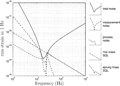
Figure 5: Noise performance of the Fabry-Perot cavity. The rms total strain noise is defined to be $[2S_{h}^{\text{tot}}/(1\ \text{second})]^{1/2}$, and all the other noise densities are normalized similarly. The equivalent one-sided bandwidth is one hertz.

As a final check, the assumption of free test mass dynamics yields the standard quantum limit (SQL)

$$S_{h}^{\text{SQL}}(\omega) \overset{\scriptscriptstyle\text{def}}{=}\lim_{1/|\tilde{G}|\to m\omega^{2}}S_{h}^{\text{tot}}(\omega)$$

$$\overset{\hskip 1.72218pt\raisebox{-1.07639pt}[0.0pt][0.0pt]{\includegraphics[width=4.73611pt]{PIMA_checkCharacter.epsf}}}{=}\frac{\hbar}{m\omega^{2}L^{2}}$$ (22)

in accord with the literature .

As shown in Fig. 5, the reference design beats the SQL in the 10–30 Hz band. But this does not signify any evasion of the rigorous quantum limits (19–21), because the SQL assumption of free test mass dynamics is not justified, viz., the dynamical kernel $\tilde{G}(\omega)$ differs greatly from the free kernel $-1/(m\omega^{2})$ in consequence of optical forces and springs.

These results illustrate a fundamental principle of field theory: all physics can be derived from the scattering matrix. In our case the scattering matrix is the optical amplitude (7a–7b), and from this sole input the path integral/measurement amplitude formalism constructs both the classical dynamics and the quantum noise.

VI Accord with the Gravity Wave Detection Literature

Now we will show that the path integral results of the preceding section—both dynamical and noise-related—accord with prior results from the gravity-wave detection community Caves (1980, 1981); Braginsky and Vyatchanin (2002); Braginsky et al. (2001a); Braginsky (1998); Buonanno and Chen (2002a, 2001a, 2001b, b); Braginsky et al. (2001b); Khalili (2001); Braginsky and Khalili (1999), which were obtained mainly by operator and field-theoretic methods.

Showing accord is daunting because the gravity-wave community has a tradition—extending back at least twenty years—of “lively controversies” Caves (1980).

Much recent discussion has been stimulated by the work of Braginsky and colleagues Braginsky et al. (2001b), who have been cited Buonanno and Chen (2001a) as showing that “the test-mass wave-function aspect of the uncertainty principle is irrelevant to the operation of a [gravity-wave] interferometer”.

To put a sharp point on the issue, how can the path integral/measurement amplitude formalism, in which the test mass is explicitly quantized but light is not, be equivalent to other—seemingly opposite—formalisms in which the test mass is not explicitly quantized but light is?

In showing that there need be no contradiction, we will build upon a seminal article by Caves Caves (1980) and an analysis of photodetection by Gardiner and Zoller Gardiner and Zoller (2000). Caves’ analysis revealed “two different, but equivalent points of view regarding the origin of … radiation-pressure fluctuations.” Seeking further equivalent points of view, we can identify in Gardiner and Zoller’s analysis (and in much other quantum optics literature) at least six variables in which quantum fluctuations occur (Table 4).

Table 4: Variables in which quantum fluctuations are commonly identified.

$\displaystyle{\bm{j}}_{\text{in}}(t)$ $\displaystyle:\ \text{the laser source current,}$ $\displaystyle{\bm{A}}_{\text{in}}(t)$ $\displaystyle:\ \text{the gauge field at the input port(s),}$ $\displaystyle{\bm{A}}_{\text{cav}}(t)$ $\displaystyle:\ \text{the gauge field within the cavity,}$ $\displaystyle{\bm{j}}_{\text{mir}}(t)$ $\displaystyle:\ \text{the mirror current,}$ $\displaystyle{\bm{A}}_{\text{out}}(t)$ $\displaystyle:\ \text{the gauge field at the output port(s),}$ $\displaystyle{\bm{j}}_{\text{out}}(t)$ $\displaystyle:\ \text{the photodiode sink.}$

Viewed as field operators, these variables are linked by Maxwell’s equations, such that fluctuations in any one operator determine the fluctuations of all the others (up to boundary conditions on the optical field). Thus, any one of these variables can reasonably serve as the focus of an “equivalent point of view” in the sense of Caves.

The path integral/measurement amplitude method amounts to a point of view that is focussed upon the test mass trajectory $q(t)$ and can be formalized as follows:

• The quantum dynamics of the mirror are embodied (4–b) in a path integral over $q(t)$.

• Maxwell’s equations are enforced by the optical kernel (IV), with $q(t)$ as the source term.

• Optical boundary conditions are specified via the measurement amplitude (IV).

Adherants of this point of view can nonetheless consistently agree with the very different point of view of Caves’ articles Caves (1980, 1981), which focus upon vacuum fluctuations at the input ports. In a measurement amplitude formalism the port fluctuations appear implicitly in the photon counting statistics of the measurement amplitude (IV), in accord with Gardiner and Zoller’s dictum Gardiner and Zoller (2000):

Under the conditions that normally apply for a practical photodetector, the ‘out’ electron field has the same statistics as the ‘in’ photon field.

Thus, vacuum fluctuations entering at the input port necessarily appear in the photon statistics. This reconciles—at least in principle—the port-oriented point of view with the path integral/measurement amplitude formalism.

This suggests the general principle that a path integral/measurement amplitude analysis should agree with any other analysis that treats at least one variable quantum mechanically, enforces Maxwell’s and Newton’s equations, and imposes compatible boundary conditions on the optical fields.

As a test of this “many viewpoints” principle, we have carried through a path integral analysis of each of the measurement schemes that were analyzed in Braginsky et al. (2001b) by operator methods; we find exact agreement between the two formalisms in all cases. This work will be reported in a separate article. However, a conceptual issue arose in which the language of control theory proved more precise than the language of physics; this precision played a key role in reconciling the two viewpoints.

The issue is: what is a free mass? To a control engineer the question is ill-posed, because an appropriate control kernel can create dynamics that are equivalent to a virtual spring, even though no physical spring is present. Conversely, a physical spring attached to a test mass can be veiled by a control kernel, such that the controlled dynamics are equivalent to those of a free mass.

Veiled springs pose a conceptual obstacle in measurement theory because they allow violation of the free-mass standard quantum limit by test masses that are only seemingly free. We found in Braginsky et al. (2001b) several examples of meters that—upon computing an equivalent measurement amplitude, path integral, and control diagram—proved quantum-mechanically equivalent to a physical spring plus a spring-veiling controller. In every case the reciprocity relation (19) was satisfied, such that violations of the standard quantum limit were due to the veiled spring.

VII Conjectured Limits to Interferometric Test Mass Observation

We set forth in this section conjectured limits that, if correct, constrain all designs for interferometric gravity wave detectors, including past and future quantum nondemolition designs. To maintain an intellectual equilibrium—and to help sustain the gravity wave community’s tradition of “lively controversy”—we will suggest in Section VIII several approaches by which these conjectures might be proved wrong or evaded.

To start, we propose the following conventional definition of a free mass:

Definition 1

A free mass is defined to have a transfer function $\tilde{\mathcal{G}}(\omega)\overset{\scriptscriptstyle\text{def}}{=}\tilde{q}(\omega)/\tilde{f}(\omega)=-1/(m\omega^{2})=1/(ms^{2})$.

Here $s$ is the Laplace variable traditionally preferred over $\omega$ by control engineers, and $\tilde{\mathcal{G}}(\omega)$ includes both mechanical and optical springs. This definition unveils hidden springs, and from a control engineering point of view is the most natural definition.

We then propose the following conjecture, which formalizes the path integral result (19):

Conjecture 1

For any stationary lossless interferometric measurement processes, the measurement noise spectral density $S_{q}(\omega)$ and the process noise spectral density $S_{f}(\omega)$ satisfy an exact equality

$$S_{q}(\omega)S_{f}(\omega)=\hbar^{2}/4$$ (23)

and these noise processes are uncorrelated.

Here the “stationary” constraint excludes stroboscopic Braginsky and Khalili (1999) and squeezed Rugar and Grütter (1991) measurements, and “lossless” is understood to mean “no unobserved decoherence.” We recall from the discussions following (2b) and (18) that the measurement noise $q_{\text{n}}(t)$ and process noise $f_{\text{n}}(t)$ are not equivalent to shot noise and radiation-pressure noise, but rather are mnemonic aids whose sole role is to remind us to include $S_{f}$ and $S_{q}$ in (2b).

The point of Conjecture 1 is to suggest that (23) need not be regarded as a limit to be approached, but instead provides us with an exact law of nature that even the most clumsily designed experiments cannot violate, provided only that all decoherence is observed and no observations are discarded. This viewpoint facilitates the informatic investigations we propose in Section VIII.

Definition 1 and Conjecture 1 lead immediately to a lemma (derived in (19–V)):

Lemma 1

For any stationary interferometric test mass measurement, the spectral density $S_{h}^{\text{tot}}(\omega)$ of the equivalent gravitational strain noise satisfies an inequality

$$S_{h}^{\text{tot}}(\omega)\geq\frac{\hbar}{m^{2}\omega^{4}L^{2}|\tilde{G}(\omega)|}$$ (24)

where $m$ is the reduced mirror mass, $L$ is the arm length, $\omega$ is the angular observation frequency, and $\tilde{G}(\omega)$ is the test mass transfer function, including optical forces.

Since this inequality—the sprung mass quantum limit—holds even for squeezed photon detection statistics (as discussed following (IV)), the point of Lemma 1 is to suggest the strong hypothesis that all stationary measurement schemes for exceeding the standard quantum limit, if analyzed from the path integral/measurement amplitude point of view, and with care taken to unveil hidden springs, are equivalent to the design strategy of the previous section, which can be formalized as follows:

• Install an optical or mechanical spring that increases $|\tilde{G}(\omega)|$ relative to the free mass value of $1/(m\omega^{2})$,

• Simultaneously tune the sideband response of the cavity to balance $S_{q}(\omega)$ and $S_{h}(\omega)$ such that the sprung mass limit (24) is saturated over the broadest feasible bandwidth, and

• Install a control kernel $\tilde{\Gamma}(\omega)$ to quench any optomechanical instabilities and—if desired—alter or veil the dynamical effects of the optical spring.

The nondemolition meters proposed in Braginsky et al. (2001b) are consistent with this strategy, but there are many other proposed meters in the literature that remain to be considered before it could be considered general.

If Lemma 1 is correct, then optimizing the sensitivity of interferometric gravity wave detectors is a problem that can be posed purely in terms of classical optomechanical design. Because the theoretical and practical limits to maximizing $\tilde{G}(\omega)$ are not known, Lemma 1 imposes no fundamental limit—quantum or classical—on the sensitivity of interferometric gravity wave detection.

VIII Discussion

Conjecture 1 and Lemma 1 are suggested by the path integral/measurement amplitude formalism, but they are far from proved. We will now outline a program by which they might be proved wrong or evaded. Beyond its intrinsic scientific interest, this program would advance at least three practical goals: quantum cryptography, single-spin imaging, and interferometric gravity-wave detection.

Quantum cryptography and quantum entanglement considerations arise naturally when we consider how to generalize the measurement amplitude (IV) to the case of multiple output ports. A natural $n$-port ansatz is

$$\exp\left[\frac{\mathcal{M}(\{r_{i}(t)\},q(t))}{i\hbar}\right]= \mbox{\raisebox{-2.15277pt}[0.0pt][0.0pt]{$\underset{i\in 1,n}{\mbox{\huge$\Pi$}}$}}\Bigg{(}\bigg{[}\frac{a_{i}(t|q(t))}{|a_{i}(t|q(t))|}\bigg{]}^{r_{i}(t)}$$

$$\times\exp\bigg{[}\frac{-(r_{i}(t)-|a_{i}(t|q(t))|^{2})^{2}}{4\alpha_{i}|a_{i}(t|q(t))|^{2}}\bigg{]}\Bigg{)}$$ (25)

where $\{a_{i}(t|q(t)),r_{i}(t),\alpha_{i}\}$ specify the amplitude functional, detection rate, and photon count squeezing at the $i$’th output port. This measurement amplitude—or a similar expression—would have to be rigorously grounded in field theory before Conjecture 1 could be regarded as a theorem. Furthermore, the design analysis of real-world gravity-wave detectors, whether analytically or by quantum numerical simulation, also requires an explicit $n$-port measurement amplitude.

The following thought experiment suggests how challenging such a field-theoretic grounding might be. Consider a four-port interferometer observing a single test mass, in which Alice monitors Ports 1 and 2 while Bob monitors Ports 3 and 4.

Alice and Bob decide—independently and secretly—how to process their ports. For example, Alice can decide to count photon rates $|a_{1}|^{2}$ and $|a_{2}|^{2}$, or alternatively she can count $|a_{1}-ia_{2}|^{2}/2$ and $|a_{1}+ia_{2}|^{2}/2$; Alice’s data records will in general be very different depending on her choice, as will her inferred values of $S_{q}(\omega)$ and $S_{f}(\omega)$.

Alice’s choices must be invisible to Bob, and Bob’s choices must be invisible to Alice; otherwise causality is violated. But depending on the quantum dynamics of the test mass, there is at least the possibility of quantum entanglement of Alice and Bob’s port amplitudes. Furthermore, Alice and Bob have the option—at least in principle—of storing their light away, for analysis at some future time by a method to be decided later; such delayed choices must also be mutually transparent.

Such thought experiments suggest that rigorously justifying or refuting (23–VIII) will encompass nontrivial issues of quantum entanglement, consistent with a recent proposal by Marshall et al. Marshall et al. (2002).

Quantum entanglement issues appear with redoubled subtlety when we consider magnetic resonance force microscopy (MRFM). As with interferometric gravity wave detection, MRFM experiments monitor test masses by optical interferometry Sidles (1992); Rugar et al. (1992); Sidles et al. (1992). Their differing physical scale—nanograms, nanowatts, and nanometers for MRFM interferometers versus kilograms, kilowatts, and kilometers for gravity wave interferometers—is not particularly relevant to the physics. More fundamentally different is the MRFM community’s goal of observing the non-classical force signal from an individual spin.

Early work in MRFM included the test mass quantum dynamics, but did not include a quantum analysis of the measurement process Sidles et al. (1992). Conversely, direct interferometric observation of a single spin has been analyzed Sidles (1996), but this “toy” analysis did not include any test mass dynamics. Thus, no integral quantum analysis of a combined interferometer/spin/test-mass system is available at present. As MRFM technology approaches attonewton force sensitivity Stowe et al. (1997), such that long-envisioned single-spin detection and bioimaging applications Sidles et al. (1992) approach feasibility, this fundamental quantum measurement challenge is gaining in urgency.

The statistical nature of the transition between spin-up and spin-down signals has crucial practical significance for the MRFM community; it strongly conditions the design of optimal signal processing algorithms. This is is a practical embodiment of a decades-old question: when and how does a quantum wave function collapse?

Similarly gaining in urgency is the practical challenge of how best to tune and operate gravity wave interferometers. For want of theoretical guidance, the interferometer of Section V was tuned empirically. Had we sent the output photons to Alice—per the discussion above—along with a homodyne reference, Alice might have achieved much better sensitivity, viz., a substantially more optimal balance between $S_{q}(\omega)$ and $S_{f}(\omega)$.

Alice’s secretly improved sensitivity has to be transparent to Bob’s simultaneous observation. Thus, part of Alice and Bob’s communication challenge is to agree on how best to establish a consensus test mass trajectory, and how best to distinguish shot noise from radiation-pressure noise in their combined data records. The resulting Alice-Bob dialog would cast new light on these contentious issues—doubly so if they were sharing nonclassical spin signals in an MRFM context.

In summary, the quantum signal processing and control challenges in both gravity wave interferometry and magnetic resonance force microscopy are mathematically well-posed, reasonably accessible via the path integral/measurement amplitude formalism, rich in fundamental physics and unexplored information-theoretic issues, and rich in quantum system engineering challenges. A new generation of instruments based on these technologies—instruments of unprecedented sensitivity, if they can be made to work—promises to open new worlds for scientific observation and exploration.