Dynamics of entanglement for coherent excitonic states in a system of two coupled quantum dots and cavity QED

Abstract

The dynamics of the entanglement for coherent excitonic states in the system of two coupled large semiconductor quantum dots ($R/a_{B}\gg 1$) mediated by a single-mode cavity field is investigated. Maximally entangled coherent excitonic states can be generated by cavity field initially prepared in odd coherent state. The entanglement of the excitonic coherent states between two dots reaches maximum when no photon is detected in the cavity. The effects of the zero-temperature environment on the entanglement of excitonic coherent state are also studied using the concurrence for two subsystems of the excitons.

I introduction

Demonstration of the existence of fast quantum algorithms [1] excited scientists to pour tremendous enthusiasm into the quantum computation and information theory. In this relatively new area, scientists not only make abstract theory, but also make efforts to find some physical systems to test and realize their ideas. A representative list includes the trapped ions [2], the liquid-state nuclear magnetic resonance [3] and the solid-state material [4].

Nanotechnology opens technological possibilities to fabricate mesoscopic devices. Semiconductor nanostructures, especially quantum dot structures, are very promising for the realization of quantum computation and the quantum information processing. The quantum gate realization using quantum dots has been proposed  [5]. Sanders et al. have discussed the scalable solid-state quantum computer based on electric dipole transitions within coupled single-electron quantum dots [6]. Imamoglu et al. propose a scheme which realizes controllable interactions between two distant quantum dot spins by combining the cavity quantum electrodynamics (QED) with electronic spin degrees in quantum dots [7]. Entanglement of the exciton states in a single quantum dot or in a quantum dot molecule has been also demonstrated experimentally [8, 9]. The reference [10] investigate the entanglement of excitonic states in the system of the optically driven coupled quantum dots theoretically and propose a method to prepare maximally entangled Bell and Greenberger-Horne-Zeilinger states. Berman et al. has investigated the dynamics of entangled states and a quantum control-not gate for an ensemble of four-spin molecules and shown that entangled states can be generated using a resonant interaction between the spin system and an electromagnetic $\pi$ pulse  [11].

The main focus of the references cited above is the entanglement of the excitonic orthogonal states. In fact, not only the entangled orthogonal states but also entangled nonorthogonal states play an important role in quantum cryptography [12] and quantum teleportation [13]. One kind of entangled nonorthogonal states is the entangled coherent states [14, 15] which can be generated by a nonlinear Mach-Zender interferometer. However up to now, no scheme for generating entangled excitonic coherent states has been proposed. This paper will focus on this topic, especially, on the dynamics of the entangled excitonic coherent states in the system of two large semiconductor quantum dots coupled by a single-mode field. The conditions for the preparation of maximally entangled excitonic states are derived assuming that the effective radius $R$ of each quantum dot is much larger than the Bohr-radius $a_{B}$ of the bulk-exciton. The interactions between two quantum dots is mediated only by the single-mode cavity field.

This paper is organized as follows: In Sec. II, we will describe the Hamiltonian of the system of interest, and obtain the solutions of the operators which present dynamical quantity. Then we will give the wave function of the system with certain initial states. In Sec. III, we will discuss the entanglement of the excitonic coherent states in the system of the two coupled quantum dots by virtue of the concurrence [16, 17]. The effects of environment on concurrence will be discussed in Sec. IV, and finally the conclusion of this study will be presented in Sec. V.

II Hamiltonian and solutions

The model that is analyzed in this study consists of two quantum dots which are placed into a single-mode cavity. The quantum dots have large sizes satisfying the condition $R\gg a_{B}$. We also assume that there are a few electrons excited from valence-band to conduction-band. Then the excitation density of the Coulomb-correlated electron-hole pairs, excitons, in the ground state for each quantum dot is low. This, in turn, implies that the average number of excitons is no more than one for an effective area of the excitonic Bohr radius. Therefore exciton operators can be approximated with boson operators, and all nonlinear terms including exciton-exciton interactions and the phase space filling effect can be neglected. The ground energy of the excitons in each dots is assumed to be the same. There is a resonant interaction between the single-mode cavity field and the excitons. The distance between two quantum dots is assumed to be much larger than the optical wavelength $\lambda$ of the cavity field, so the interaction between quantum dots can be neglected. Under the rotating wave approximation, the Hamiltonian for this system can be written as [18]

$$H_{0}=\hbar\omega\hat{a}^{\dagger}\hat{a}+\hbar\omega\sum_{m=1}^{2}\hat{b}^{\dagger}_{m}\hat{b}_{m}+\hbar\sum_{m=1}^{2}g_{m}(\hat{b}^{\dagger}_{m}\hat{a}+\hat{a}^{\dagger}\hat{b}_{m})$$ (1)

where $\hat{a}^{\dagger}(\hat{a})$ are the operators of the cavity field with frequency $\omega$, $\hat{b}^{\dagger}_{m}(\hat{b}_{m})$ denote the exciton operators with the same frequency $\omega$ of the cavity field, and $m=1(2)$ represent the first dot or the second dot. The coupling constants between quantum dot one (two) and cavity field are represented by $g_{m}$ with $m=1,2$. Without loss of generality, we can take the two coupling constants between the cavity field and the quantum dots as different. The Heisenberg equations of motion for the operators of the cavity field $\hat{a}(\hat{a}^{\dagger})$ and the excitons $\hat{b}_{m}(\hat{b}^{\dagger}_{m})$ can be easily obtained as

$$\frac{\partial\hat{a}}{\partial t} = -i\omega\hat{a}-ig_{1}\hat{b}_{1}-ig_{2}\hat{b}_{2}$$ (3)

$$\frac{\partial\hat{b}_{1}}{\partial t} = -i\omega\hat{b}_{1}-ig_{1}\hat{a}$$ (4)

$$\frac{\partial\hat{b}_{2}}{\partial t} = -i\omega\hat{b}_{2}-ig_{2}\hat{a}$$ (5)

It is very easy to obtain the solutions of the above operator equations as

$$\hat{a}(t)=\cos(gt)\hat{a}(0)e^{-i\omega t}-i\frac{g_{1}}{g}\sin(gt)\hat{b}_{1}(0)e^{-i\omega t}$$ (7)

$$-i\frac{g_{2}}{g}\sin(gt)\hat{b}_{2}(0)e^{-i\omega t}$$ (8)

$$\hat{b}_{1}(t)=-i\frac{g_{1}}{g}\sin(gt)\hat{a}(0)e^{-i\omega t}+\frac{g_{1}^{2}\cos(gt)+g_{2}^{2}}{g^{2}}\hat{b}_{1}(0)e^{-i\omega t}$$ (9)

$$+\frac{g_{1}g_{2}[\cos(gt)-1]}{g^{2}}\hat{b}_{2}(0)e^{-i\omega t}$$ (10)

$$\hat{b}_{2}(t)=-i\frac{g_{2}}{g}\sin(gt)\hat{a}(0)e^{-i\omega t}+\frac{g_{1}g_{2}[\cos(gt)-1]}{g^{2}}\hat{b}_{1}(0)e^{-i\omega t}$$ (11)

$$+\frac{g_{2}^{2}\cos(gt)+g_{1}^{2}}{g^{2}}\hat{b}_{2}(0)e^{-i\omega t}$$ (12)

with $g=\sqrt{g_{1}^{2}+g_{2}^{2}}$.

We assume that the cavity field is initially prepared in a superposition of two distinct coherent states $|\alpha_{1}\rangle$ and $|\alpha_{2}\rangle$ in the normalized form of

$$|\psi(0)\rangle_{c}=C|\alpha_{1}\rangle+D|\alpha_{2}\rangle.$$ (13)

The two modes of excitons are in the vacuum states $|0\rangle_{1}|0\rangle_{2}$ with label $1(2)$ denoting exciton mode one (two). The whole initial state for the excitons and the cavity field can be expressed as

$$|\Psi(0)\rangle=(C|\alpha_{1}\rangle+D|\alpha_{2}\rangle)\otimes|0\rangle_{1}|0\rangle_{2}.$$ (14)

The time dependent wave function $|\Psi(t)\rangle$ of the whole system can use the time evolution operator $U(t)=e^{-i(Ht/\hbar)}$ and initial state $|\Psi(0)\rangle$ to express as $|\Psi(t)\rangle=U(t)|\Psi(0)\rangle$, that is

$$|\Psi(t)\rangle=U(t)(C|\alpha_{1}\rangle+D|\alpha_{2}\rangle)\otimes|0\rangle_{1}|0\rangle_{2}.$$ (15)

According to the definition of the coherent state, any coherent state of the cavity field has the following form

$$|\alpha\rangle=\exp[\alpha\hat{a}^{\dagger}(0)-\alpha^{*}\hat{a}(0)]|0\rangle$$ (16)

where ($\ast$) denotes complex conjugation. Then (15) can be rewritten as

$$|\Psi(t)\rangle = U(t)[C\exp(\alpha_{1}\hat{a}^{\dagger}(0)-\alpha_{1}^{*}\hat{a}(0))$$ (17)

$$+ D\exp(\alpha_{2}\hat{a}^{\dagger}(0)-\alpha_{2}^{*}\hat{a}(0))]|0\rangle|0\rangle_{1}|0\rangle_{2}.$$ (18)

We may interpolate unit operator $U^{\dagger}(t)U(t)$ into Eq.(18) and consider the properties of the time evolution operator $U^{\dagger}(t)OU(t)=O(t)$ and $U(t)|0\rangle=|0\rangle$, then Eq.(18) becomes as

$$|\Psi(t)\rangle = C|\alpha_{1}u(t)\rangle\otimes|\alpha_{1}v_{1}(t)\rangle_{1}\otimes|\alpha_{1}v_{2}(t)\rangle_{2}$$ (19)

$$+ D|\alpha_{2}u(t)\rangle\otimes|\alpha_{2}v_{1}(t)\rangle_{1}\otimes|\alpha_{2}v_{2}(t)\rangle_{2}$$ (20)

with

$$u(t) = \cos(gt)e^{-i\omega t},$$ (22)

$$v_{1}(t) = -i\frac{g_{1}}{g}\sin(gt)e^{-i\omega t},$$ (23)

$$v_{2}(t) = -i\frac{g_{2}}{g}\sin(gt)e^{-i\omega t}.$$ (24)

For convenience, we will drop the time dependence $t$ from $u(t)$, $v_{1}(t)$, and $v_{2}(t)$ in the following expressions. It is very clear that three subsystems become entangled with the time evolution except at some critical times $t=n\pi/2g$ for integer $n$. But what we are interested in is the entanglement between two subsystems of excitons, so we trace over mode of the cavity field in the density matrix of the system given as $|\Psi(t)\rangle\langle\Psi(t)|$ to obtain the reduced density matrix $\rho(t)={\rm Tr}(|\Psi(t)\rangle\langle\Psi(t)|)$ of excitons for any arbitrary time $t$. This partial trace operation enables us to describe the dynamics of the excitons in the coupled quantum dot system without any reference to the cavity field. Then the reduced density matrix $\rho(t)$ is found as

$$\rho(t) = [C^{*}D{\cal N}(|\alpha_{2}v_{1}\rangle\langle\alpha_{1}v_{1}|)_{1}\otimes(|\alpha_{2}v_{2}\rangle\langle\alpha_{1}v_{2}|)_{2}+h.c.]$$ (25)

$$+ |C|^{2}(|\alpha_{1}v_{1}\rangle\langle\alpha_{1}v_{1}|)_{1}\otimes(|\alpha_{1}v_{2}\rangle\langle\alpha_{1}v_{2}|)_{2}$$ (26)

$$+ |D|^{2}(|\alpha_{2}v_{1}\rangle\langle\alpha_{2}v_{1}|)_{1}\otimes(|\alpha_{2}v_{2}\rangle\langle\alpha_{2}v_{2}|)_{2}.$$ (27)

Here $h.c.$ denotes complex conjugate. ${\cal N}$ is an inner product of two coherent states $|\alpha_{2}u\rangle$ and $|\alpha_{1}u\rangle$, and ${\cal N}=\exp\left[-\cos^{2}(gt)(\frac{1}{2}|\alpha_{1}|^{2}+\frac{1}{2}|\alpha_{2}|^{2}-\alpha^{*}_{1}\alpha_{2})\right]$. It is evident that unitary evolution of the wave function cannot change its purity, however tracing out the cavity field reduces the other subsystems into a statistical mixture.

III entanglement of excitonic states

Concurrence is a useful tool to measure entanglement between two subsystems of $2\times 2$ biparte mixed and pure states. According to the references [16, 17], we assume that $1$ and $2$ is a pair of qubits, and the density matrix of the pair is $\rho_{12}$. Then the concurrence of the density matrix $\rho_{12}$ is defined as:

$${\cal C}_{12}=max\{\lambda_{1}-\lambda_{2}-\lambda_{3}-\lambda_{4},0\}$$ (28)

where $\lambda_{1}$, $\lambda_{2}$, $\lambda_{3}$, and $\lambda_{4}$ given in decreasing order are the square roots of eigenvalues for matrices

$$M_{12}=\rho_{12}(\sigma_{1y}\otimes\sigma_{2y})\rho^{*}_{12}(\sigma_{1y}\otimes\sigma_{2y})$$ (29)

with Pauli matrix

$$\sigma_{1y}=\left(\begin{array}[]{cc}0&-i\\ i&0\end{array}\right);\hskip 14.22636pt\sigma_{2y}=\left(\begin{array}[]{cc}0&-i\\ i&0\end{array}\right),$$ (30)

and ($\ast$) denoting complex conjugation in the standard basis $\{|00\rangle,|01\rangle,|10\rangle,|11\rangle\}$, and $\sigma_{1y}$ and $\sigma_{2y}$ are expressed in the same basis. The entanglement of formation is a monotonically increasing function of ${\cal C}_{12}$. ${\cal C}_{12}=0$ corresponds to an unentangled state, and ${\cal C}_{12}=1$ corresponds to a maximally entangled state.

First, we make a suitable transformation on Eq.(27) so that we can define the qubit and discuss the entanglement between two modes of excitons using the concurrence. We can choose two different coherent states, which are nonorthogonal and form a super-complete set, as a basis to span a two-dimensional Hilbert space. But it is not suitable to define qubits using two-dimensional super-complete set of basis. However, one can always rebuild two orthogonal and normalized states as basis of the two-dimensional Hilbert space using original two coherent states [19]. In our system, we can choose two time-dependent excitonic coherent states to define qubits. We define the zero qubit state as $|0\rangle_{m}=|\alpha_{1}v_{m}(t)\rangle$; and one qubit state as $|1\rangle_{m}=(|\alpha_{2}v_{m}(t)\rangle-\langle\alpha_{1}v_{m}(t)|\alpha_{2}v_{m}(t)\rangle|\alpha_{1}v_{m}(t)\rangle)/N_{m}(t)$ with $N_{m}(t)=\sqrt{1-|\langle\alpha_{1}v_{m}(t)|\alpha_{2}v_{m}(t)\rangle|^{2}}=\sqrt{1-P_{m}^{2}(t)}$ for exciton systems of mode one $m=1$ and two $m=2$. The above definition for qubits is equivalent to the definition in reference [20]. In this new basis, the reduced density matrix (27) can be rewritten into

$$\rho = \{C^{*}D{\cal N}[(N_{1}(t)|1\rangle\langle 0|)_{1}+P_{1}(t)(|0\rangle\langle 0|)_{1}]\otimes$$ (35)

$$[(N_{2}(t)|1\rangle\langle 0|)_{2}+P_{2}(t)(|0\rangle\langle 0|)_{2}]+h.c.\}$$

$$|D|^{2}[(N_{1}(t)|1\rangle+P_{1}(t)|0\rangle)(N^{*}_{1}(t)\langle 1|+P_{1}^{*}(t)\langle 0|)]_{1}\otimes$$

$$[(N_{2}(t)|1\rangle+P_{2}(t)|0\rangle)(N^{*}_{2}(t)\langle 1|+P^{*}_{2}(t)\langle 0|)]_{2}$$

$$+|C|^{2}(|0\rangle\langle 0|)_{1}\otimes(|0\rangle\langle 0|)_{2}.$$

For simplicity, we assume that two quantum dots are completely the same so that the interaction between cavity field and two quantum dots are equal to each other, that is $g_{1}=g_{2}$. We consider the cases where the cavity field is initially prepared in the even or odd coherent states. It has been shown that such mesoscopic coherent superpositions can be generated by experimentalists using cavity QED [21] or a trapped ion [22]. For the cavity field initially prepared in the odd coherent state, Eq.(13) can be written as

$$|odd\rangle=N_{-}(|\alpha\rangle-|-\alpha\rangle)$$ (36)

with normalization constant $N_{-}=(2-2e^{-2|\alpha|^{2}})^{-\frac{1}{2}}$. Under the above conditions, we can write $N_{1}(t)=N_{2}(t)=M=\sqrt{1-P^{2}(t)}$ and $P=P_{1}(t)=P_{2}(t)=e^{-\sin^{2}(gt)|\alpha|^{2}}$. Then the reduced density operator (35) can be rewritten in the matrix representation as follows

$$R(\rho)=\frac{1}{2(1-e^{-2|\alpha|^{2}})}\left(\begin{array}[]{cccc}1-2{\cal N}P^{2}+P^{4}&-{\cal N}MP+MP^{3}&-{\cal N}MP+MP^{3}&-{\cal N}M^{2}+M^{2}P^{2}\\ -{\cal N}MP+MP^{3}&M^{2}P^{2}&M^{2}P^{2}&M^{3}P\\ -{\cal N}MP+MP^{3}&M^{2}P^{2}&M^{2}P^{2}&M^{3}P\\ -{\cal N}M^{2}+M^{2}P^{2}&M^{3}P&M^{3}P&M^{4}\end{array}\right)$$ (37)

in the standard basis $\{|00\rangle,|01\rangle,|10\rangle,|11\rangle\}$ where every basis vector such as $|00\rangle$ denotes state $|0\rangle_{1}\otimes|0\rangle_{2}$. We can obtain the square roots of eigenvalues of the matrix (29) corresponding to the matrix (37) as

$$\lambda_{1} = \frac{(1-e^{-2\sin^{2}(gt)|\alpha|^{2}})(1+e^{-2\cos^{2}(gt)|\alpha|^{2}})}{2(1-e^{-2|\alpha|^{2}})}$$ (39)

$$\lambda_{2} = \frac{(1-e^{-2\sin^{2}(gt)|\alpha|^{2}})(1-e^{-2\cos^{2}(gt)|\alpha|^{2}})}{2(1-e^{-2|\alpha|^{2}})}$$ (40)

$$\lambda_{3} = \lambda_{4}=0.$$ (41)

Then the concurrence $C_{o}$ of the prepared state with an initial odd coherent state of the cavity field is found as

$$C_{o}=\frac{e^{-2\cos^{2}(gt)|\alpha|^{2}}(1-e^{-2\sin^{2}(gt)|\alpha|^{2}})}{(1-e^{-2|\alpha|^{2}})}.$$ (42)

We can also obtain the average photon number $\bar{n}$ of the cavity field as follows

$$\bar{n}=\langle a^{\dagger}a\rangle=\frac{|\alpha|^{2}\cos^{2}(gt)(1+e^{-2|\alpha|^{2}})}{1-e^{-2|\alpha|^{2}}}.$$ (43)

Eqs.(42-43) show that two subsystems of the excitons becomes maximally entangled for any time satisfying the condition $gt=(n+\frac{1}{2})\pi$ for any intensity $|\alpha|^{2}$ of the coherent cavity field, and in this moment no photon of the cavity field can be detected. Fig. 1 shows the time evolution of (42) for two different intensity values $|\alpha|^{2}$ of the cavity field. It is clearly seen that maximally entangled coherent states of excitons can be prepared by the cavity field of odd coherent states. The entanglement periodically reaches its maximum. It is also found that when the excitonic states are in a maximally entangled state, the average photon number of the cavity field is zero (see Fig.3). This enables us to monitor the status of the system during preparation of the entangled excitonic coherent states by detecting the photon number of the cavity field.

If the cavity field is initially prepared in an even coherent state

$$|even\rangle=N_{+}(|\alpha\rangle+|-\alpha\rangle)$$ (44)

where the normalization constant is $N_{+}=(2+2e^{-2|\alpha|^{2}})^{-\frac{1}{2}}$, using the same procedure the concurrence $C_{e}$ is found as

$$C_{e}=\frac{e^{-2\cos^{2}(gt)|\alpha|^{2}}(1-e^{-2\sin^{2}(gt)|\alpha|^{2}})}{(1+e^{-2|\alpha|^{2}})},$$ (45)

and the average number $\bar{n}$ of the cavity field is

$$\bar{n}=\langle a^{\dagger}a\rangle=\frac{|\alpha|^{2}\cos^{2}(gt)(1-e^{-2|\alpha|^{2}})}{1+e^{-2|\alpha|^{2}}}.$$ (46)

From Eq.(45), it is found that we can not obtain maximally entangled states when the cavity field is initially in the even coherent state. But the analytical expression (45) shows that when the coherent intensity $|\alpha|$ of the cavity field tends to infinity, we can approximately obtain maximally entangled excitonic coherent state at

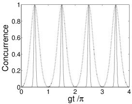
FIG. 1.: Time evolution of the concurrence $C_{o}$ is plotted as a function of $\frac{gt}{\pi}$ for (a) $|\alpha|=1$ (dashed), (b) $|\alpha|=5$ (solid).

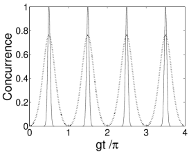
FIG. 2.: Time evolution of the concurrence $C_{e}$ is plotted as a function of $gt/\pi$ for (a) $|\alpha|=1$ (dashed), (b) $|\alpha|=5$ (solid).

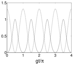
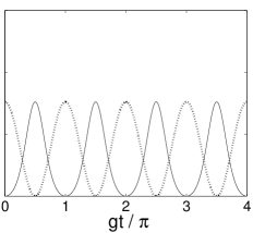
FIG. 3.: Time evolutions of the concurrence (solid curve) and average photon number $\bar{n}$ (dashed curve) are plotted as a function of $gt/\pi$ for cavity field initially prepared with $|\alpha|=1$ as odd coherent state (left) and even coherent state (right).

time $gt=(n+\frac{1}{2})\pi$. In fact numerical results show that when the coherent intensity $|\alpha|\geq 2$, the concurrence approximately reaches its maximum at the same time $gt=(n+\frac{1}{2})\pi$. Fig.2 shows the time evolution of the concurrence $C_{e}$ for two different $|\alpha|$ values of the cavity field. It is concluded that a quasi-maximally entangled excitonic coherent states can be prepared using the initial even coherent state of the cavity field when the coherent intensity $|\alpha|$ becomes intensive.

In Fig.3, a comparison of the degree of entanglement and its relation with the average number of photons ($\bar{n}$) in the cavity for cavity fields initially prepared in odd and even coherent states is presented. It is seen that (i) Both the concurrence and $\bar{n}$ shows a periodic evolution, (ii)Concurrence reaches to its maximum value when $\bar{n}=0$ for both cases, and (iii) for the cavity field initially prepared in odd coherent state, it is possible to obtain maximally entangled states for some evolution times, but this is not true for cavity field initially prepared in even coherent state.

IV effect of environment on the entanglement of excitons

In this section, we will focus our attention on how the environment with zero temperature affects the entanglement of the excitons. We assume that the energy of the system is dissipated only by the interaction of the excitons in the quantum dots with the multi-modes of electromagnetic radiation. Our discussion is limited to these two completely equivalent quantum dots, that is, they have the same coupling constants with the cavity field, and also have the same dissipative dynamics. Under above considerations, we have the following Hamiltonian with the rotating-wave approximation as

$$H = H_{0}+\hbar\sum_{m=1}^{2}\sum_{k}\omega_{m,k}a^{\dagger}_{m,k}a_{m,k}$$ (47)

$$+ \sum_{m=1}^{2}\sum_{m,k}\kappa_{m,k}(a_{m,k}b^{\dagger}_{m}+a^{\dagger}_{m,k}b_{m})$$ (48)

where $H_{0}$ is determined by (1), and $a^{\dagger}_{m,k}(a_{m,k})$ denote the multi-modes electromagnetic field operators with the frequencies $\omega_{m,k}$, and $m=1(2)$ means the quantum dot one (two). Using the assumption $g_{1}=g_{2}=\kappa=g/\sqrt{2}$, and $\kappa_{1,k}=\kappa_{2,k}$, we can write the equations of motion for all operators as follows

$$\frac{\partial\hat{a}}{\partial t}=-i\omega_{0}\hat{a}-i\kappa\hat{b}_{1}-i\kappa\hat{b}_{2},$$ (50)

$$\frac{\partial\hat{b}_{m}}{\partial t}=-i\omega_{0}\hat{b}_{m}-i\kappa\hat{a}-i\sum_{k}\kappa_{m,k}a_{m,k},$$ (51)

$$\frac{\partial a_{m,k}}{\partial t}=-i\omega_{m,k}a_{m,k}-i\kappa_{m,k}b_{m}.$$ (52)

We know that only the solution of the cavity field operator is enough to solve our problem. We apply the Laplace transformation and the Wigner-Weisskopf approximation [23] to the above set of Eqs.(50-52). So the time-dependent solution of the cavity field operator with the zero-temperature environment can be obtained as

$$a(t) = u^{\prime}(t)a(0)+v^{\prime}_{1}(t)b_{1}(0)+v^{\prime}_{2}(t)b_{2}(0)$$ (53)

$$+ \sum_{k}v_{1,k}(t)a_{1,k}(0)+\sum_{k}v_{2,k}(t)a_{2,k}(0)$$ (54)

where

$$u^{\prime}(t) = \frac{e^{-\frac{\gamma}{4}t}[\gamma(e^{\frac{i}{4}\Delta t}-e^{-\frac{i}{4}\Delta t})+i\Delta(e^{\frac{i}{4}\Delta t}+e^{-\frac{i}{4}\Delta t})]e^{-i\omega t}}{i2\Delta}$$ (56)

$$v_{1}^{\prime}(t) = v_{2}^{\prime}(t)=\frac{2\kappa[e^{\frac{1}{4}(-\gamma+i\Delta)t}-e^{\frac{1}{4}(-\gamma-i\Delta)t}]e^{-i\omega t}}{i\Delta}$$ (57)

with $\Delta=\sqrt{32\kappa^{2}-\gamma^{2}}$, and $\gamma=2\pi\epsilon(\omega_{0})|\kappa(\omega_{0})|^{2}$ where $\epsilon(\omega)$ is a distribution function of the multimode electromagnetic radiation field. A small Lamb frequency shift has been neglected in above Eqs.(56-57). We take the same steps as in the Sect. II, and obtain the time-dependent wave function of the whole system with cavity field initially in the odd mesoscopic coherent superposition of states (36) and other subsystems in the vacuum states

$$|\Psi(t)\rangle=C|\alpha u^{\prime}(t)\rangle\otimes\prod_{m=1}^{2}|\alpha v^{\prime}_{m}(t)\rangle\otimes\prod_{m=1}^{2}\prod_{k}|\alpha v_{m,k}(t)\rangle$$ (58)

$$-C|-\alpha u^{\prime}(t)\rangle\otimes\prod_{m=1}^{2}|-\alpha v^{\prime}_{m}(t)\rangle\otimes\prod_{m=1}^{2}\prod_{k}|-\alpha v_{m,k}(t)\rangle.$$ (59)

After tracing over the environment and the cavity field, we obtain the reduced density matrix of two subsystems of the excitons as

$$\rho^{\prime}_{o}(t) = [|C|^{2}{\cal N}^{\prime}(|\alpha_{2}v^{\prime}_{1}\rangle\langle\alpha^{\prime}_{1}v_{1}|)_{1}\otimes(|\alpha_{2}v^{\prime}_{2}\rangle\langle\alpha_{1}v^{\prime}_{2}|)_{2}+h.c.]$$ (60)

$$+ |C|^{2}(|\alpha_{1}v^{\prime}_{1}\rangle\langle\alpha_{1}v^{\prime}_{1}|)_{1}\otimes(|\alpha_{1}v^{\prime}_{2}\rangle\langle\alpha_{1}v^{\prime}_{2}|)_{2}$$ (61)

$$+ |C|^{2}(|\alpha_{2}v^{\prime}_{1}\rangle\langle\alpha_{2}v^{\prime}_{1}|)_{1}\otimes(|\alpha_{2}v^{\prime}_{2}\rangle\langle\alpha_{2}v^{\prime}_{2}|)_{2}$$ (62)

with ${\cal N}^{\prime}=e^{-|\alpha|^{2}(1-2|v^{\prime}_{1}|^{2})}$, where the condition $\sum_{k}|v_{1,k}(t)|^{2}+\sum_{k}|v_{2,k}(t)|^{2}=1-|u^{\prime}(t)|^{2}-|v^{\prime}_{1}(t)|^{2}-|v^{\prime}_{2}(t)|^{2}$, which comes from the commutation relation $[a(t),a^{\dagger}(t)]=1$, is used. Then we choose the basis as the section II, and use the same step to obtain the concurrence corresponding to the reduced density matrix operator (62)

$$C^{\prime}_{o}=\frac{e^{-2|\alpha|^{2}(1-2|v^{\prime}_{1}|^{2})}(1-e^{-4|\alpha|^{2}|v^{\prime}_{1}|^{2}})}{(1-e^{-2|\alpha|^{2}})},$$ (63)

where $v^{\prime}_{1}$ is determined by (57). When $\gamma=0$ which means that the whole system has no any dissipation of energy, then we find that (63) returns to ideal case (42). Figs. 4 and 5 show that the entanglement of the two coherent excitonic states is gradually reduced by the environment with time evolution. If the decay rate $\gamma$ of the excitons is fixed, then the higher the intensity of the cavity field is, the faster the decay of entanglement is. In the same way, if the intensity of the cavity field is fixed, then for a system with larger decay rate $\gamma$ of excitons, the amount of entanglement reduces faster.

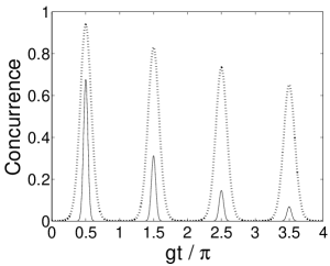
FIG. 4.: Time evolution of the concurrence $C_{o}$ is plotted as a function of $gt/\pi$ for $\gamma/g=0.01$ when $|\alpha|=5$ (solid), and $|\alpha|=2$ (dashed).

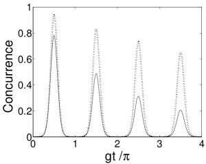
FIG. 5.: Time evolution of the concurrence $C_{o}$ is plotted as a function of $gt/\pi$ for $\gamma/g=0.01$ (dashed), and $\gamma/g=0.04$ (solid) when $|\alpha|=2$.

V Conclusion

The entanglement of formation for coherent states of the excitons in the system of two coupled quantum dots by cavity field is investigated. We find that a maximally entangled coherent state of two-modes excitons can be prepared by an odd coherent state of the cavity field. The status of this entangled excitonic coherent state can be probed by the measurement of the cavity field. No photon detection in the cavity implies the preparation of maximally entangled excitonic coherent states. In the case of photon detection of any number, it can be said that the excitons are not maximally entangled.

The effects of the zero-temperature environment on the entanglement of excitons is also studied by using concurrence. It is found that the amount of entanglement between two excitonic coherent states is reduced by the environment with time evolution due to the loss of photons of the cavity field to the environment. If leakage from the cavity to the environment is monitored by photon counting detectors, an absence of photo-detections implies that maximally entangled state of the excitons can be found in the coupled quantum dot system with time evolution. In case of any photon detection, we are certain that the system can not reach to a maximally entangled state. If the decay rate $\gamma$ of the excitons is given, for the system with higher cavity field intensity, the decrease in the amount of entanglement is faster. It is also understood that if the coherent intensity of the cavity field is given, then the large decay rate $\gamma$ of excitons corresponds to a fast reduction in entanglement of the system.

To have an idea on the characteristic time-scales of the dynamics of entanglement in our model, we can take $\hbar g\simeq 0.5~{}{\rm meV}$ which may be possible to obtain in a system of large area quantum dot with cavity [7]. In that case, for an ideal cavity with initial field prepared as an odd coherent state, the first maximally entangled state could be observed after a time evolution of $2~{}{\rm ps}$ and this would repeat itself periodically with a period of $4~{}{\rm ps}$. For a practical cavity, the finite cavity lifetime may be taken as $\gamma^{-1}\simeq 10~{}{\rm ps}$ [7]. For these $g$ and $\gamma$ values, we can find $\gamma/g\simeq 0.13$. With $|\alpha|=2$ ($|\alpha|=1$), the maximum value for concurrence would be $\sim 0.46$ ($\sim 0.8$)which occurs at $t\simeq 2~{}{\rm ps}$. After a time evolution of $4~{}{\rm ps}$, the second peak for the concurrence would appear with a value of $\sim 0.17$ ($\sim 0.53$). It is clearly seen that for a practical scheme the main parameters which would affect the dynamics of the system are the fast rate of the photon loss from the cavity and intensity of the initial cavity field.

VI Acknowledgments

The authors thank to A. Miranowicz for helpful discussions. Y. L. is grateful to the Japan Society for the Promotion of Science (JSPS) for support. This work is also supported by Grant-in-Aid for Scientific Research (B) (Grant No. 12440111) by Japan Society for the Promotion of Science.

REFERENCES

- [1] P. W. Shor, Proc. of the 35th Annual Symposium on the Foundations of Computer Science, edited by Goldwasser, (IEEE Computer Society, Los Alamitos, CA, 1994), p.124; L. K. Grover, Phys. Rev. lett. 79, 325(1997).
- [2] J. I. Cirac and P. Zoller, Phys. Rev. Lett. 74, 4091(1995); A. Sorensen and K. Molmer, Phys. Rev. Lett. 82, 1971(1999).
- [3] N. A. Gershenfeld and I. L. Chuang, Science 275, 350(1997); I. L. Chuang, L. M. K. Vandersypen, X. Zhou, D. W. Leung and S. Lloyd, Nature 393, 143(1998).
- [4] K. Obermayer, G. Mahler, and H. Haken, Phys. Rev. Lett. 58, 1792(1987).
- [5] A. Barenco, D. Deutsh, and A. Ekert, and R. Jozsa, Phys. Rev. Lett. 74, 4083(1995); D. Loss and P. DiVincenzo, Phys. Rev. A57, 120(1998); S. Bandyopadhyay, Phys. Rev. B 61, 13813(2000); Tetsufumi Tanamoto, Phys. Rev. A 61, 022305(2000); Xuedong Hu, and S. Das Sarma, Phys. Rev. A 61, 062301(2000).
- [6] G. D. Sanders, K. W. Kim, and W. C. Holton, Phys. Rev. A 61, 7526(2000).
- [7] A. Imamolu, D. D. Awschalom, G. Burkard, D. P. DiVincenzo, D. Loss, M. Sherwin, and A. Small, Phys. Rev. Lett. 83, 4204 (1999); Mark S. Sherwin, A. Imamolu, and Thomas Montroy, Phys. rev. A 60, 3508(1999).
- [8] G. Chen, N. H. Bonadeo, D. G. Steel, D. Gammon, D. S. Katzer, D. Park, L. J. Sham, Science 289, 1906 (2000).
- [9] M. Bayer, P. Hawrylak, K. Hinzer, S. Fafard, M. Korkusinski, Z. R. Wasilewski, O. Stern, and A. Forchel, Science 291, 451 (2001).
- [10] L. Quiroga, and N. F. Johnson, Phys. Rev. Lett. 83, 2270 (1999); J. H. Reina, L. Quiroga, and N. F. Johnson, Phys. Rev. A62, 012305 (2000).
- [11] G. P. Berman, G. D. Doolen, G. V. López, and V. I. Tsifrinovich, Phys. Rev. B 58, 11570(1998); G. P. Berman, G. D. Doolen, R. Mainieri, and V. I. Tsifrinovich, Introduction to Quantum Computers (World Scientific, Singapore, 1998).
- [12] Christopher A. Fuchs, Phys. Rev. Lett. 79, 1162(1997).
- [13] Xiaoguang Wang, quant-ph/0102011, Xiaoguang Wang, quant-ph/0102048 (will be published in Phys. Rev. A).
- [14] B. C. Sanders, Phys. Rev. A 45, 6811(1992), A. Mann, B. C. Sanders, W. J. Munro, Phys. Rev. A 51, 989(1995).
- [15] S. J. van Enk, O. Hirota, Phys. Rev. A 64, 022313(2001).
- [16] Scott Hill and William K. Wotters, Phys. Rev. Lett. 78, 5022(1997); William K. Wotters, Phys. Rev. Lett. 80, 2245(1998).
- [17] V. Coffman, J. Kundu, and William K. Wootters, Phys. Rev. A 61, 052306(2000).
- [18] E. Hanamura, Phys. Rev. B 38, 1228(1988); L. Belleguie and L. Banyai, Phys. Rev. B 44, 8785(1991); H. Cao, S. pau, Y. Yamamoto, and Björk, Phys. Rev. B54, 8083(1996).
- [19] Dipanker Home and M. K. Samal, quant-ph/0012064.
- [20] H. Jeong, M. S. Kim, and Jinhyoung Lee, Phys. Rev. A 64, 052308(2001).
- [21] S. Haroche, Phys. Today 51(7), 36(1998); M. Brune, F. Hagley, J. Dreyer, X. Maitre, A. Maali, C. Wunderlich, J. M. Raimond, and S. Haroche, Phys. Rev. Lett. 77, 4887(1996).
- [22] C. Monroe, D. M. Meekhof, B. E. king, and D. J. Wineland, Science 272, 1131(1996).
- [23] W. H. Louisell, Quantum Statistical Properties of Radiation, (John Wiley & Sons, New York, 1990).