A Robust Method for Estimating the Lindblad Operators of a Dissipative Quantum Process from Measurements of the Density Operator at Multiple Time Points

Abstract

We present a robust method for quantum process tomography, which yields a set of Lindblad operators that optimally fit the measured density operators at a sequence of time points. The benefits of this method are illustrated using a set of liquid-state Nuclear Magnetic Resonance (NMR) measurements on a molecule containing two coupled hydrogen nuclei, which are sufficient to fully determine its relaxation superoperator. It was found that the complete positivity constraint, which is necessary for the existence of the Lindblad operators, was also essential for obtaining a robust fit to the measurements. The general approach taken here promises to be broadly useful in studying dissipative quantum processes in many of the diverse experimental systems currently being developed for quantum information processing purposes.

I Introduction

An important task in designing and building devices capable of quantum information processing (QIP) is to determine the superoperators that describe the evolution of their component subsystems from experimental measurements. This task is commonly known in QIP as Quantum Process Tomography (QPT) NielsenChuang . The superoperators obtained from QPT allow one to identify the dominant sources of decoherence and focus development efforts on eliminating them, while precise knowledge of relevant parameters can be used to design quantum error correcting codes the and/or decoherence-free subsystems that circumvent their effects BouwmEkertZeili ; NielsenChuang . Methods have previously been described by which the “superpropagator” $\mathcal{P}$ of a quantum process can be determined Childs ; Fujiwara . Assuming that the process’ statistics are stationary and Markovian Alicki ; Weiss , a more complete description may be obtained by determining the corresponding “supergenerator”, that is, a time-independent superoperator $\mathcal{G}$ from which the superpropagator at any time $t$ is obtained by solving the differential equation $\dot{\mathcal{P}}(t)=-\mathcal{G}\,\mathcal{P}(t)$. The formal solution to this equation is $\exp(-\mathcal{G}t)$, where “$\exp$” is the operator exponential.

The purpose of this paper is to describe a data fitting procedure by which estimates of a supergenerator can be obtained. This problem is nontrivial because, as in many other data fitting problems, the estimates obtained from straightforward (e.g. least-squares) fits turn out to be very sensitive to small, and even random, errors in the measured data. In some cases, this may result in a supergenerator that is obviously physically impossible; in others, it may simply result in large errors in the generator despite it yielding a reasonably good fit to the data. Parameter estimation problems with this property are commonly known as ill-conditioned RoussLeroy ; Tarantola . The main result of this paper is that, although the problem of estimating a supergenerator from measurements of the superpropagators at various times is ill-conditioned, this ill-conditioning can be greatly alleviated by incorporating prior knowledge of the solution into the fitting procedure as a constraint. The prior knowledge that we use here is a very general property of open quantum system dynamics known as complete positivity.

Roughly speaking, complete positivity means that if $\mathcal{P}$ is a superoperator that maps a density operator of a system to another density operator, then any extension of the form $\mathcal{I}\otimes\mathcal{P}$ also returns a positive operator, where $\mathcal{I}$ denotes the identity map on the extension of the domain. The most general form of a completely-positive Markovian master equation for the density operator $\rho$ of a quantum system is known as the Lindblad equation Alicki ; Weiss . This may be written as

$$\dot{\rho}(t)~{}=~{}-\imath[H,\,\rho(t)]\,+\,\tfrac{1}{2}\,\sum_{m=1}^{M}\,\big{(}[L_{m}\,\rho(t),\;L_{m}^{\dagger}]\,+\,[L_{m},\;\rho(t)\,L_{m}^{\dagger}]\big{)}~{},$$ (1)

where $\hbar=1$, $t$ is time, $H$ is the system’s Hamiltonian, the $L_{m}$ are known as Lindblad operators, and the $L_{m}^{\dagger}$ denote their adjoints. It is easily seen that the Lindblad equation necessarily preserves the trace $\mathrm{tr}(\rho)=1$ of the density matrix, meaning  $\mathrm{tr}(\dot{\rho})=0$, and a little harder to show that it also preserves the positive-semidefinite character of the density operator. Proofs that it has the yet-stronger property of complete positivity may be found in Refs. Alicki ; Lindblad ; GorKosSud ; HavelPre . The QPT method we describe in this paper relies upon the Lindblad characterization of complete positivity.

The paper is organized as follows. In the first part of the paper we present a computational procedure which fits a completely positive supergenerator to a sequence of estimates of the superpropagators of a quantum process at multiple time points. This procedure initially extracts an estimate of the decoherent part of the supergenerator, without the Hamiltonian commutation superoperator (which is assumed to be available from independent prior measurements). It then refines this initial estimate via a nonlinear least-squares fit to the superpropagators, in which complete positivity is enforced by adding a suitable penalty function to the sum of squares minimized. Finally, any residual non-completely-positive part of the supergenerator is “filtered” out by a matrix projection technique based on principle component analysis HavelPre ; Jollife .

In the second part of the paper, the procedure is validated by using it to determine the natural spin-relaxation superoperator of a molecule containing two coupled spin $1/2$ nuclei in the liquid state from a temporal sequence of density operators. These in turn were derived by state tomography, meaning a set of NMR measurements sufficient to determine the density matrix. In the process we confirm the ill-conditioned nature of the problem, and that the complete positivity constraint is needed to obtain a robust estimate of the supergenerator. The final results are used to compute the corresponding Lindblad operators, but these were difficult to interpret. Hence the Hadamard representation of $T_{2}$-relaxation dynamics HavHad was used to derive a new set of Lindblad operators which are easier to interpret and explain most of the relaxation dynamics. The information these operators convey agree with theoretical expectations as well as with some additional independent measurements, in support of the accuracy of the results obtained.

II Computational procedure

In this paper we are concerned with an $N$-dimensional open quantum system ($N<\infty$), the dynamics of which are described by a Markovian master equation of the form Ernst ; Weiss ; Alicki :

$$\begin{split}\frac{\mathrm{d}\rho}{\mathrm{d}t}=&-\imath\,[H,\,\rho\,]\,-\,\mathcal{R}\,(\rho-\rho_{\textsf{eq}})\\[3.0pt] \Leftrightarrow~{}\frac{\mathrm{d}\rho_{\Delta}}{\mathrm{d}t}=&-\imath\,\mathcal{H}\,\rho_{\Delta}\,-\,{\mathcal{R}}\,\rho_{\Delta}\end{split}$$ (2)

In this equation, $\hbar\equiv 1$, $\rho=\rho(t)$ is the system’s density operator, $\rho_{\textsf{eq}}$ this operator at thermal equilibrium, $\rho_{\Delta}\equiv\rho-\rho_{\textsf{eq\,}}$, $H$ is the system’s internal Hamiltonian, $\mathcal{H}$ the corresponding commutation superoperator, and $\mathcal{R}$ is the so-called relaxation superoperator. The equivalence of the first and second lines follows from the fact that $\rho_{\textsf{eq}}$ is time-independent and proportional to the Boltzman operator $\exp(-H/k_{\textsf{B}}T)$, so that it commutes with $H$.

By choosing a basis for the “Liouville space” of density operators, the equation may be written in matrix form as Ernst ; HornJohn ; HavelPre

$$\frac{\mathrm{d}|{\underline{\,\smash{\rho}}_{\Delta}}\rangle}{\mathrm{d}\hskip 0.50003ptt}~{}=~{}-\big{(}\imath\,\underline{\mathcal{H}}\,+\,\underline{{\mathcal{R}}}\,\big{)}|{\underline{\,\smash{\rho}}_{\Delta}}\rangle~{}\equiv~{}-\underline{\mathcal{G}}\,|{\underline{\,\smash{\rho}}_{\Delta}}\rangle$$ (3)

where the underlines denote the corresponding matrices and $|{\underline{\,\smash{\rho}}}\rangle$ is the $N^{2}$-dimensional column vector obtained by stacking the columns of the density matrix $\underline{\,\smash{\rho}}$ on top of each other in left-to-right orderHavelPre . A numerical solution to this equation at any point $t$ in time may be obtained by applying the propagator $\underline{\mathcal{P}}(t)$ to the initial condition $|{\underline{\,\smash{\rho}}_{\Delta}(0)}\rangle$, where the propagator is obtained by computing the matrix exponential $\underline{\mathcal{P}}(t)=\underline{\smash{\exp}}\big{(}\!-\!\underline{\mathcal{G}}\,t\hskip 0.50003pt\big{)}$ HornJohn ; NajHav . Note that $\underline{\mathcal{H}}$ and $\underline{\mathcal{R}}$ do not commute in general, and that the sum $\underline{\mathcal{G}}\equiv\imath\,\underline{\mathcal{H}}+\underline{\mathcal{R}}$ will not usually be a normal matrix (one which commutes with its adjoint). This in turn greatly reduces the efficiency and stability with which its matrix exponential can be computed Moler+vanLoan (although this was not an issue in the small problems dealt with here), and we expect it to also significantly complicate the inverse problem.

In this section we describe an algorithm for solving this inverse problem, that is to determine the relaxation superoperator $\underline{\mathcal{R}}$ from an estimate of the Hamiltonian $\underline{H}$ together with estimates of the propagator $\underline{\mathcal{P}\!}_{\,m}=\underline{\mathcal{P}}(t_{m})$ at one or more time points $t_{1}<t_{2}<\ldots<t_{M}$. This problem, like many other inverse problems, turns out to be ill-conditioned, meaning that small experimental errors in the estimates of the $\underline{H}$ and $\underline{\mathcal{P}\!}_{\,m}$ may be amplified to surprisingly large, and generally nonphysical, errors in the resulting superoperator $\underline{\mathcal{R}}$ RoussLeroy . For example, if one tries to estimate $\underline{\mathcal{R}}$ in the obvious way as

$$\underline{\mathcal{R}}~{}\approx~{}\Big{(}-\imath\,\underline{\mathcal{H}}\,-\,\underline{\smash{\log}}\big{(}\underline{\mathcal{P}\!}_{\,1}\big{)}\Big{)}\Big{/}t_{1}~{},$$ (4)

one will generally obtain nonsense even if $\underline{\mathcal{H}}$ and $\underline{\mathcal{P}\!}_{\,1}$ are known to machine precision, because of the well-known ambiguity of the matrix logarithm with respect to the addition of independent multiples of $2\,\imath\,\pi$ onto its eigenvalues. Using the principal branch of the logarithms will only work if $\mathcal{H}$ is small compared to ${\mathcal{R}}$, and the only reasonably reliable means of resolving the ambiguities is to utilize additional data and/or prior knowledge of the solution. Even then, a combinatorial search for the right multiples of $2\,\imath\,\pi$ may be infeasibly time-consuming.

An alternative to the logarithm which utilizes data at multiple time points and is capable of resolving the ambiguities even when $\mathcal{H}$ is much larger than ${\mathcal{R}}$ is to estimate the derivative at $t=0$ of

$$\underline{e}^{it\underline{\mathcal{H}}/2}\,\underline{\mathcal{P}}(t)\,\underline{e}^{it\underline{\mathcal{H}}/2}~{}=~{}\underline{e}^{-t\,\underline{\mathcal{R}}}\,+\,O(t^{2})~{}.$$ (5)

This derivative is obtained by Richardson extrapolation using central differencing about $t=0$ over a sequence of time points such that $t_{m}=2^{m-1}t_{1}$ ($m=1,\ldots,M$), according to the well-known procedure DahlBjor :

for $m$ from $1$ to $M$ do
	$\underline{\mathcal{D}}_{\,1,1+M-m}~{}:=~{}2^{m-2\,}\big{(}\underline{e}^{it_{m}\underline{\mathcal{H}}/2}\,\underline{\mathcal{P}\!}_{\,m}\,\underline{e}^{it_{m}\underline{\mathcal{H}}/2}\,-\,\underline{e}^{-it_{m}\underline{\mathcal{H}}/2}\,\underline{\mathcal{P}\!}_{\,m}^{\;-1}\,\underline{e}^{-it_{m}\underline{\mathcal{H}}/2}\big{)}\,$;
	for $\ell$ from $1$ to $m-1$ do
		$\underline{\mathcal{D}}_{\,1+\ell,1+M-m}~{}:=~{}\underline{\mathcal{D}}_{\,\ell,1+M-m}\,+\,(\underline{\mathcal{D}}_{\,\ell,1+M-m}\,-\,\underline{\mathcal{D}}_{\,\ell,M-m})/(4^{\ell}-1)\,$;
	end do
end do

The inverse $\underline{\mathcal{P}\!}_{\,m}^{\;-1}=\underline{\mathcal{P}}(-t_{m})$ is assured of existing unless long times are used or the errors in the data are large. The method produces an estimate of the derivative at $t=0$ that is accurate up to $O(t_{\,1}^{\,2M})$, and which may be increased by computing the exponential from the highest-order estimate at further interval halvings. The method performs well when the relative errors in the Hamiltonian $\delta\ll 1/(\Delta\nu\,t_{M})$, where $\Delta\nu$ is the range of frequencies present in the Hamiltonian, but it tends to emphasize the errors in $\underline{\mathcal{P}\!}_{\,1}$ rather than averaging over the errors at all the time points. Hence we do not recommend that it be used alone, but rather as a means of obtaining a good starting point for a nonlinear fit to the data, as will now be described.

This nonlinear fit involves minimization of the sum of squares

$$\chi^{2}\big{(}\underline{\mathcal{R}};\,\underline{\mathcal{H}},\underline{\mathcal{P}\!}_{\,1\,},\ldots,\underline{\mathcal{P}\!}_{\,M}\big{)}~{}\equiv~{}\sum_{m=1}^{M}\,\Big{\|}\,\underline{\smash{\exp}}\big{(}-\!(\imath\,\underline{\mathcal{H}}+\underline{\mathcal{R}})\,t_{m}\,\big{)}\;-\;\underline{\mathcal{P}\!}_{\,m}\Big{\|}^{2}_{\textsf{F}}$$ (6)

with respect to $\underline{\mathcal{R}}$, where $\|\cdot\|^{2}_{\textsf{F}}$ denotes the squared Frobenius norm (sum of squares of the entries of its matrix argument). Previous results with similar minimization problems indicate that $\chi^{2}$ will have many local minima Kwaku , making a good starting point absolutely necessary (even disregarding the $2\imath\pi$ ambiguities discussed above). The derivatives of this function may be obtained via the techniques described in Ref. NajHav , but the improvements in efficiency to be obtained by their use are likely to be of limited value in practice given that all the resources needed, both experimental and computational, grow rapidly with $N$ (which itself grows exponentially with the number of qubits used in quantum information processing problems). In addition, the quality of the results matters a great deal more than the speed with which they are obtained, and the quality will not generally depend greatly on the accuracy with which the minimum is located.

For these reasons, we have used the Nelder-Mead simplex algorithm NeldMead , as implemented in the MATLAB^TM program, for the small (two qubit) experimental test problem described in the following section. This has the further advantage of being able to avoid local minima better than most gradient-based optimization algorithms. Preliminary numerical studies, however, exhibited the anticipated ill-conditioning with respect to small perturbations in the data, even when $\underline{\mathcal{R}}$ was constrained to be symmetric (implying a unital system which satisfies detailed balance) and positive semidefinite (as required for the existence of a finite fixed point). Therefore it is necessary to incorporate additional prior information regarding $\underline{\mathcal{R}}$ into the minimization. The information that we have found to be effective is a property of $\underline{\mathcal{R}}$ known as complete positivity Weiss ; Alicki ; HavelPre .

An intrinsic definition which does not involve an environment was first given by Kraus Kraus2 , and states that a superpropagator $\mathcal{P}$ is completely positive if and only if it can be written as a “Kraus operator sum”, namely

$$\mathcal{P}(\rho)~{}=~{}\sum_{\ell=1}^{N^{2}}\,K_{\rule{0.0pt}{4.37012pt}\ell}\,\rho\,K_{\ell}^{\dagger}~{},$$ (7)

where $\rho=\rho^{\dagger}$ and $K_{1},\ldots,K_{N^{2}}$ all act on the system alone. Another intrinsic definition subsequently given by Choi Choi states that a superpropagator is completely positive if and only if, relative to any basis of the system’s Hilbert space, the so-called Choi matrix is positive semidefinite HavelPre , namely

$$\underline{0\rule[-1.29167pt]{0.0pt}{0.0pt}}~{}\preceq~{}\underline{C\rule[-0.86108pt]{0.0pt}{0.0pt}}~{}\equiv~{}\sum_{i,j=0}^{N-1}\,\underline{\mathcal{P}\smash{(|{\hskip 0.5pti\hskip 0.5pt}\rangle\langle{j}|)}}\otimes(|{\hskip 0.5pti\hskip 0.5pt}\rangle\langle{j}|)~{}=~{}\sum_{i,j=0}^{N-1}\,\underline{\mathcal{P}\rule[-0.86108pt]{0.0pt}{0.0pt}}(|{\hskip 0.5pti\hskip 0.5pt}\rangle|{j}\rangle)(\langle{\hskip 0.5pti\hskip 0.5pt}|\langle{j}|)~{}.$$ (8)

This equation uses the notation of quantum information processing, in which the $i$-th elementary unit vector is denoted by $|{\hskip 0.5pti\hskip 0.5pt}\rangle$ ($0\leq i<N$), $\underline{\mathcal{P}\smash{(|{\hskip 0.5pti\hskip 0.5pt}\rangle\langle{j}|)}}$ is the $N\times N$ matrix of the operator obtained by applying the superpropagator $\mathcal{P}$ to the projection operator given by $|{\hskip 0.5pti\hskip 0.5pt}\rangle\langle{j}|$ versus our choice of basis, and $\underline{\mathcal{P}\rule[-0.86108pt]{0.0pt}{0.0pt}}$ is the $N^{2}\times N^{2}$ matrix for $\mathcal{P}$ versus the Liouville space basis $|{\hskip 0.5pti\hskip 0.5pt}\rangle|{j}\rangle$ (as for $\underline{\mathcal{H}}$ etc. above). It can further be shown that the eigenvectors $\underline{k}_{\,\ell}$ of the Choi matrix are related to the (matrices of an equivalent set of) Kraus operators by $|{\underline{K\!}_{\,\ell}}\rangle=\sqrt{\kappa_{\ell}}\,\underline{k}_{\ell\,}$, where $\kappa_{\ell}\geq 0$ are the corresponding eigenvalues and the “ket” $|{\underline{K\!}_{\,\ell}}\rangle$ indicates the column vector obtained by stacking the columns of $\underline{K\!}_{\,\ell}$ on top of one another HavelPre .

These results can be used not only to compute a Kraus operator sum from any completely positive superpropagator given as a “supermatrix” acting on the $N^{2}$-dimensional Liouville space, but also to “filter” such a supermatrix so as to obtain the supermatrix of the completely positive superpropagator nearest to it, in the sense of minimizing the Frobenius norm of their difference HavelPre . This is done simply by setting any negative eigenvalues of the Choi matrix to zero, rebuilding it from the remaining eigenvalues and vectors, and converting this reconstructed Choi matrix back to the corresponding supermatrix. Although this generally has a beneficial effect upon the least-squares fits versus $\chi^{2}$ (as defined above), it is still entirely possible that the sequence of filtered propagators ${\mathcal{P}\,}_{\!m}^{\prime}$ will not correspond to a completely positive Markovian process, so that no time-independent relaxation superoperator ${\mathcal{R}}$ can fit it precisely. This, together with the ill-conditioned nature of the problem, implies one will still not usually obtain satisfactory results even after filtering. For this reason we shall now describe how the above characterizations of completely positive superpropagators can be extended to supergenerators.

As indicated in the Introduction, completely positive Markovian processes, or quantum dynamical semigroups as they are also known, may be characterized as those with a generator $\mathcal{G}$ that can be written in Lindblad form GorKosSud ; Lindblad ; Weiss ; Alicki ; HavelPre . On expanding the commutators in Eq (1), this becomes

$$-\mathcal{G}(\,\rho\,)~{}\equiv\,-\imath\big{[}H,\,\rho\,\big{]}\;+\;\tfrac{1}{2}\,\sum_{m=1}^{N^{2}}\,\Big{(}2\,L_{m\rule{0.0pt}{4.2194pt}}\,\rho\,L_{m}^{\dagger}\,-\,L_{m}^{\dagger}L_{m\rule{0.0pt}{4.2194pt}}\,\rho\,-\,\rho\,L_{m}^{\dagger}L_{m\rule{0.0pt}{4.2194pt}}\Big{)}~{}.$$ (9)

The operators $L_{m}$ are usually called Lindblads. It may be seen that the Choi matrix $\underline{\mathcal{C}}$ associated with $-\underline{\mathcal{R}}$ is never positive semidefinite, because $\langle{\underline{I}}|\,\underline{\mathcal{C}}\,|{\underline{I}}\rangle=\mathrm{tr}(-\underline{\mathcal{R}})<0$. Nevertheless, it can be shown that any trace-preserving $\underline{\mathcal{R}}$ (meaning $\mathrm{tr}(\underline{\mathcal{R}}(\underline{\smash{\rho}}))=0$) is completely positive if and only if a certain projection of $\underline{\mathcal{C}}$ is positive semidefinite, namely $\underline{\mathcal{E}}\,\underline{\mathcal{C}}\,\underline{\mathcal{E}}$ where $\underline{\mathcal{E}}=\underline{I}\otimes\underline{I}-|{\underline{I}}\rangle\,\langle{\underline{I}}|\;$ HavelPre . In this case an equivalent system of orthogonal Lindblads is determined by $|{\underline{L}_{m}}\rangle~{}=~{}\sqrt{\lambda_{m}}\,\underline{\ell}_{\,m\,}$, where $\lambda_{m}\geq 0$ are the eigenvalues and $\underline{\ell}_{m}$ the eigenvectors of $\underline{\mathcal{E}}\,\underline{\mathcal{C}}\,\underline{\mathcal{E}}$. In the event that $\underline{\mathcal{E}}\,\underline{\mathcal{C}}\,\underline{\mathcal{E}}$ has negative eigenvalues we can simply set them to zero to obtain a similar but completely positive supergenerator, much as we did with the Kraus operators. Most importantly, however, this characterization of completely positive supergenerators gives us a means of enforcing complete positivity during nonlinear fits to a sequence of propagators at multiple time points.

The following section describes our experience with applying this approach to a sequence of propagators obtained from liquid-state NMR data. The complete positivity of the relaxation superoperator was maintained by adding a simple penalty function onto the sum of squares that was minimized by the simplex algorithm, as described above. This penalty function consisted of the sum of the squares of the negative eigenvalues of the corresponding projected Choi matrix. While more rigorous and efficient methods of enforcing the projected Choi matrix to be positive semidefinite are certainly possible, this strategy was sufficient to demonstrate the main result of this paper, which is that the complete positivity constraint greatly alleviates the ill-conditioned nature of such fits.

III Experimental Validation

The experiments were carried out on a two-spin $\frac{1}{2}$ system consisting of the hydrogen atoms in 2,3-dibromothiophene (see Fig. 1) at $300K$ dissolved in deuterated acetone, using a Bruker Avance 300 MHz spectrometer.

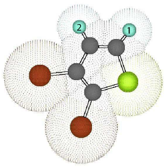
Figure 1: Molecule of 2,3-dibromothiophene with the two protons labeled $1$ and $2$. The chemical bonds among the atoms are indicated by double parallel lines, and a transparent “dot-surface” used to indicate their van der Waals radii.

The internal Hamiltonian of this system in a frame rotating at the frequency of the second spin is

$$H~{}\equiv~{}H_{int}~{}=~{}\pi\,(\,\nu_{1}\,\sigma_{\textsf{z}}^{1}\;+\;\tfrac{J}{2}\,\sigma^{1}\cdot\sigma^{2}\,)$$ (10)

where $\nu_{1}=161.63$Hz is the chemical shift of the first spin, $J=5.77$Hz is the coupling between the spins, and $\sigma=[\sigma_{\textsf{x}},\,\sigma_{\textsf{y}},\sigma_{\textsf{z}}]$ are Pauli spin operators.

The “quantum operation” we characterized was just free-evolution of the system under its internal Hamiltonian, together with decoherence and relaxation back towards the equilibrium state $\rho_{\textsf{e}q}\sim\,\sigma_{\textsf{z}}^{1}+\sigma_{\textsf{z}}^{2}$. In liquid-state NMR on small organic molecules like dibromothiophene, this process is mediated primarily by fluctuating dipolar interactions between the two protons as well as with spins neighboring molecules, and since the correlation time for small molecules in room temperature liquids is on the order of picoseconds, the Markovian approximation is certainly valid Ernst ; Freeman . We add that our sample was not degassed so that the presence of dissolved paramagnetic $O_{2}$ shortened the $T_{1}$ and $T_{2}$ relaxation times.

The experiment consisted of preparing a complete set of orthogonal input states (that is, density matrices), letting each evolve freely for a given time $T$, and then determining the full output states via quantum state tomography Chuang3 ; CoryGroup . Since only “single quantum” coherences can be directly observed in NMR Ernst ; Freeman , this involves repeating the experiment several times followed by a different readout pulse sequence each time, until all the entries of the density matrix have been mapped into observable ones. The experiments were carried out at four exponentially-spaced times $T$, as required by the Richardson extrapolation procedure described above, specifically $T=0.4,~{}0.8,~{}1.6$ and $3.2$s.

index	operator	order	index	operator	order
$1$	$4\!\times\!4$ identity	$0$	$9$	$\sigma_{\textsf{x}}^{2}$	$1$
$2$	$\sigma_{\textsf{z}}^{1}$	$0$	$10$	$\sigma_{\textsf{y}}^{2}$	$1$
$3$	$\sigma_{\textsf{z}}^{2}$	$0$	$11$	$\sigma_{\textsf{x}}^{1}\sigma_{\textsf{z}}^{2}$	$1$
$4$	$\sigma_{\textsf{z}}^{1}\sigma_{\textsf{z}}^{2}$	$0$	$12$	$\sigma_{\textsf{y}}^{1}\sigma_{\textsf{z}}^{2}$	$1$
$5$	$\sigma_{\textsf{x}}^{1}\sigma_{\textsf{x}}^{2}+\sigma_{\textsf{y}}^{1}\sigma_{\textsf{y}}^{2}$	$0$	$13$	$\sigma_{\textsf{z}}^{1}\sigma_{\textsf{x}}^{2}$	$1$
$6$	$\sigma_{\textsf{x}}^{1}\sigma_{\textsf{y}}^{2}-\sigma_{\textsf{y}}^{2}\sigma_{\textsf{x}}^{1}$	$0$	$14$	$\sigma_{\textsf{z}}^{1}\sigma_{\textsf{y}}^{2}$	$1$
$7$	$\sigma_{\textsf{x}}^{1}$	$1$	$15$	$\sigma_{\textsf{x}}^{1}\sigma_{\textsf{x}}^{2}-\sigma_{\textsf{y}}^{1}\sigma_{\textsf{y}}^{2}$	$2$
$8$	$\sigma_{\textsf{y}}^{1}$	$1$	$16$	$\sigma_{\textsf{x}}^{1}\sigma_{\textsf{y}}^{2}+\sigma_{\textsf{y}}^{1}\sigma_{\textsf{x}}^{2}$	$2$

Table 1:  Table of operators (versus Cartesian basis) in the transition basis used for the density and superoperator matrices, the corresponding matrix indices and their coherence orders (see text).

To describe the density and superoperator matrices, the so-called “transition basis” was used Ernst . This Liouville space basis is intermediate between the Cartesian basis and the Zeeman (or polarization and shift operator Ernst ) basis, in that the basis elements are all Hermitian like those of the Cartesian basis, but like the Zeeman basis they have a well-defined coherence order, or difference in total angular momentum along the applied magnetic field $B_{0}$ between the two Zeeman states connected by the transition. These basis states are listed in TABLE I versus the Cartesian basis.

This basis was chosen because the relaxation superoperator ${\mathcal{R}}$ is expected to have the “Redfield kite” structure in this basis Ernst . This block diagonal structure arises because the difference in frequency between transitions of different coherence orders, given that the Zeeman interaction dominates all others, is large enough to average out these other interactions including those responsible for decoherence and relaxation, in effect decoupling the blocks from one another so that no cross relaxation occurs between them (see Fig. 2).

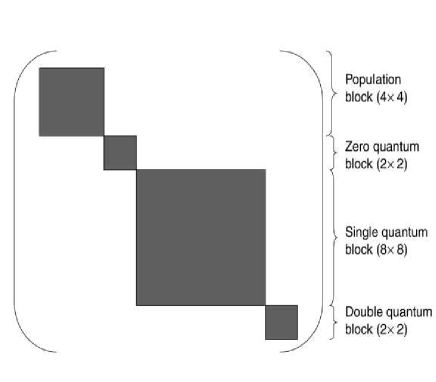
Figure 2: Redfield kite struture of the relaxation superoperator expressed in the transition basis. The non-shaded area corresponds to Blocks of different coherence order are decoupled from each other.

This so-called “secular approximation” considerably reduces the number of parameters in the superoperator from $256=((2^{2})^{2})^{2}$ to $81=3^{2}+2^{2}+8^{2}+2^{2}$ (since neither the identity nor the other diagonal ($\sigma_{\textsf{z}}$) basis elements are expected to cross relax with any non diagonal elements).

An additional reduction may be obtained by assuming detailed balance: the microscopic reversibility of all cross relaxation processes. The relaxation superoperator reconstructed from the experimental data was bordered with an initial row and column of zeros to force $\mathcal{R}(\,I\,)=0$, because the totally random density matrix $I/4$ cannot be observed by NMR spectroscopy and because of the trace-preserving process assumption that we made. This may be done providing $\mathcal{R}$ operates on $\rho_{\Delta}=\rho-\rho_{\mathsf{eq}}$, and together with detailed balance it implies that the supermatrix $\underline{\mathcal{R}}$ will be symmetric, reducing the number of parameters to be estimated to only $48=6+3+36+3$.

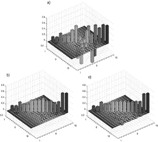
Figure 3: Three different estimates of the relaxation superoperator of $2,3$-dibromothiophene in the transition basis, indexed as indicated in Table I. (a) Relaxation superoperator obtained from a least-squares fit, without the complete positivity constraint, of the exponential $\underline{\smash{\exp}}(-\imath(\underline{\mathcal{H}}+\underline{\mathcal{R}})t_{m})$ to the propagators $\underline{\mathcal{P}}_{m}$ at the corresponding times ($t_{1}=0.4,t_{2}=0.8,t_{3}=1.6,t_{4}=3.2$s) with respect to the unknown relaxation superoperator $\underline{\mathcal{R}}$, starting from the results of Richardson extrapolation (see text). (b) The relaxation superoperator obtained from a fit to the same data and with the same starting value of $\underline{\mathcal{R}}$, but with the complete positivity constraint included in the fit. (c) The relaxation superoperator obtained by assuming that $\mathcal{H}$ and $\mathcal{R}$ commute, and using the average of the estimates obtained by taking the logarithms of the absolute values of the eigenvalues of the propagators over all four time points as the final estimate (see text).

The result of applying the fitting procedure without the complete positivity constraint to the initial estimate obtained by Richardson extrapolation is shown in FIG. 3(a). It may be seen that the rates did not vary in a systematic fashion with the coherence order, and that large cross-relaxation rates were found, which is not consistent with the physics of spin relaxation in liquid-state NMR spectroscopy. In addition, this relaxation superoperator implies that spin $1$ has a $T_{2}\approx 2.3s$ while spin $2$ has a $T_{2}\approx 4.6$s, in disagreement with the independent measurements of $T_{2}$ given below.

The fit after adding the complete positivity constraint is shown in FIG. 3(b), again starting from the results of Richardson extrapolation. It may now be seen that the results do vary systematically with coherence number, and that the resulting relaxation superoperator is very nearly diagonal. To obtain further evidence for the validity of this superoperator, we measured the single spin $T_{1}$ (longitudinal, or $\sigma_{\textsf{z}}$) and $T_{2}$ (transverse, or $\sigma_{\textsf{x}}=\sigma_{\textsf{y}}$) relaxation rates, using the well-established inversion-recovery and CPMG experiments Freeman . The results for both spins were $T_{1}=5.6$s and $T_{2}=2.7$s, which agree quite well with the values of $5.6s$ and $2.6s$ obtained from this relaxation superoperator. Although this is obviously a relatively simple relaxation superoperator, it is reasonable to expect that a complete positivity constraint will substantially improve the estimates of more complicated superoperators containing nonzero cross-relaxation rates that cannot be obtained from standard experiments.

Finally, the cross-relaxation rate between the population terms $\sigma_{\textsf{z}}^{1}$ and $\sigma_{\textsf{z}}^{2}$, which is due to the well-known nuclear Overhauser effect Solomon , is essentially zero in Fig. 3(b). This can occur when the overall rotational correlation time of the molecule plus its “solvent-cage” is on the order of $1$ns, but was somewhat unexpected given the small size of $2,3$-dibromothiophene. As a result, we carried out the selective inversion recovery experiment that consists of inverting selectively the longitudinal magnetization of one of the two protons and looking at the evolution of the magnetization of the other one while the first relaxes towards thermal equilibrium. The change in longitudinal magnetization of the second proton was measured to be less than $1\%$ of the unperturbed magnetization essentially revealing no NOE effect and providing yet further evidence for the validity of this superoperator. The discrepancy between this result and the one given in Freeman is explained by the presence of dissolved paramagnetic $O_{2}$ in our sample so that the $T_{1}$ relaxation time was shortened in such a way that the NOE effect became almost unobservable (our $T_{1}$ was measured to be $5.6s$ while the $T_{1}$ reported in Freeman is around $47.5s$).

Because of the substantial degeneracy of the diagonal elements with the same coherence order, the superoperator in Fig. 3(b) was also very nearly diagonal in the eigenbasis of the Hamiltonian commutation superoperator $\mathcal{H}$, so that $\mathcal{H}$ and $\mathcal{R}$ very nearly commute. This allowed further estimates to be obtained directly from the superpropagators $\underline{\mathcal{P}}_{\,m}\approx\underline{\smash{\exp}}(-\imath\underline{\mathcal{H}}t_{m})\,\underline{\smash{\exp}}(-\underline{\mathcal{R}}t_{m})$, simply by taking the (real) logarithms of the absolute values of their eigenvalues and thereby cancelling the phase factors from the Hamiltonian’s exponential. From FIG. 3(c) we see that the result of averaging these estimates over all four evolution times is very similar to the completely positive estimate in FIG. 3(b) (correlation coefficient $0.80$; squared norms of difference over average $0.90$). We note that the estimate in FIG. 3(c) did not explicitly assume the Redfield kite structure, thereby providing a further consistency check on our results.

IV Interpretation via Lindblad and Hadamard Operators

In this section we present a system of Lindblad operators which act on the density operator to give essentially the same derivative as the relaxation superoperator described above (see FIG. 3). As described in the foregoing “Computational Procedure” section, such a system of Lindblad operators may be obtained by diagonalizing the corresponding projected Choi matrix, although it will be seen that a more easily interpreted system was obtained by considering the parts of $\mathcal{R}$ responsible for $T_{1}$ and $T_{2}$ relaxation separately and by using the so-called ”Hadamard relaxation matrix” formalism HavHad . Because these calculations were somewhat involved, however, the details of the Hadamard operators calculations are given in an appendix. We add that from here on, the relaxation superoperator $\mathcal{R}$ will refer to the matrix shown in FIG. 3(b).

These representations of relaxation processes are normally applied to the density matrix in the Zeeman basis $\underline{\smash{\rho}}_{\Delta}^{\textsf{zee}}$ (regarded as the computational basis in QIP), which requires converting the supergenerator $\mathcal{R}$ from the transition to the Zeeman basis. This is easily done via a unitary transformation, $\underline{\mathcal{R}}^{\textsf{zee}}~{}\equiv~{}2\,\underline{U}\,\underline{\mathcal{R}}^{\textsf{tra}}\,\underline{U}^{\dagger}$, where $\underline{U}\,|{\underline{\smash{\rho}}^{\textsf{tra}}}\rangle=|{\underline{\smash{\rho}}^{\textsf{zee}}}\rangle$ (the matrix $\underline{U}$ may be derived from TABLE I; the factor of $2$ corrects for a change in norm due to the fact that the transition basis is Hermitian). Although any relaxation superoperator can be modified to act directly on the density operator $\rho$ rather than its difference with the equilibrium density operator $\rho_{\Delta}=\rho-\rho_{\mathsf{eq}}$ (vide supra) by taking the right-projection $\underline{\mathcal{R}}\,\big{(}\underline{\mathcal{I}}\,-\,|{\underline{\rho}}\rangle_{\mathsf{eq}}\langle{\underline{\mathcal{I}}}|\big{)}$ Levante ; Ghose , this makes only a negligible change to $\mathcal{R}$ since in liquid-state NMR $\rho_{\textsf{eq}}$ differs from the identity $I$ by $\lesssim\!10^{-5}$. For that reason, the treatment of $T_{1}$ relaxation given below was considerably simplified by treating it as a unital (identity preserving) process acting on $\rho_{\Delta}$.

As described following Eq. (9), a complete system of Lindblad operators may be obtained by diagonalizing the projected Choi matrix

$$\underline{\mathcal{E}}\,\underline{\mathcal{C}}\,\underline{\mathcal{E}}~{}=~{}\underline{V}\,\underline{\Lambda}\,\underline{V}^{\dagger}~{},$$ (11)

where it is assumed the eigenvalues have been ordered such that $\lambda_{m}\geq\lambda_{m+1}$ for $m=1,\ldots,N^{2}-1$, and defining the Lindblad matrices such that for all $\lambda_{m}>0$:

$$|{\,\underline{L}_{m}\,}\rangle~{}=~{}\sqrt{\lambda_{m}}\,\underline{V}\,|{m}\rangle~{}.$$ (12)

This gave rise to a total of $11$ Lindblads, the phases of which were chosen so as to make them as nearly Hermitian as possible. Once this was done, all $11$ were within $2$% of being Hermitian.

The relative contributions of these Lindblads to the overall relaxation of the spins can be quantified by the squared Frobenius norms $\|\underline{L}_{m}\|_{\textsf{F}}^{2}=\lambda_{m}$. This calculation shows that about $35$% of the mean-square noise resided in the first Lindblad,

$$\underline{L}_{1}~{}\approx~{}0.346\,\big{(}\underline{\sigma}_{\textsf{z}}^{1}+\underline{\sigma}_{\textsf{z}}^{2}\big{)}\,+\,0.025\,\underline{\sigma}_{\textsf{z}}^{1}\underline{\sigma}_{\textsf{z}}^{2}~{},$$ (13)

which represents strongly correlated dephasing with a $T_{2}$ for both spins of $\sim 4.2$s HavHad , much as expected. The next four largest Lindblads together contributed, roughly equally, another $43$% to the total mean square noise, but were considerably more difficult to interpret:

$$\underline{L}_{2}~{}\approx~{} \begin{aligned} &-0.013\,\underline{\sigma}_{\textsf{x}}^{1}\,-\,0.045\,\underline{\sigma}_{\textsf{y}}^{2}\,-\,0.153\,\underline{\sigma}_{\textsf{x}}^{2}\,-\,0.061\,\underline{\sigma}_{\textsf{y}}^{2}\\ &\qquad\,+\,0.150\,\underline{\sigma}_{\textsf{x}}^{1}\underline{\sigma}_{\textsf{z}}^{2}\,-\,0.039\,\underline{\sigma}_{\textsf{y}}^{1}\underline{\sigma}_{\textsf{z}}^{2}\,+\,0.111\,\underline{\sigma}_{\textsf{z}}^{1}\underline{\sigma}_{\textsf{x}}^{2}\,+\,0.106\,\underline{\sigma}_{\textsf{z}}^{1}\underline{\sigma}_{\textsf{y}}^{2}\end{aligned}$$

$$\underline{L}_{3}~{}\approx~{} +0.046\,\underline{\sigma}_{\textsf{z}}^{1}\,-\,0.026\,\underline{\sigma}_{\textsf{z}}^{2}\,-\,0.057\,\underline{\sigma}_{\textsf{x}}^{1}\underline{\sigma}_{\textsf{y}}^{2}\,-\,0.266\,\underline{\sigma}_{\textsf{z}}^{1}\underline{\sigma}_{\textsf{z}}^{2}$$ (14)

$$\underline{L}_{4}~{}\approx~{} \begin{aligned} &-0.024\,\underline{\sigma}_{\textsf{x}}^{1}\,-\,0.006\,\underline{\sigma}_{\textsf{y}}^{2}\,-\,0.081\,\underline{\sigma}_{\textsf{x}}^{2}\,-\,0.077\,\underline{\sigma}_{\textsf{y}}^{2}\\ &\qquad\,-\,0.155\,\underline{\sigma}_{\textsf{x}}^{1}\underline{\sigma}_{\textsf{z}}^{2}\,-\,0.193\,\underline{\sigma}_{\textsf{y}}^{1}\underline{\sigma}_{\textsf{z}}^{2}\,+\,0.002\,\underline{\sigma}_{\textsf{z}}^{1}\underline{\sigma}_{\textsf{x}}^{2}\,-\,0.012\,\underline{\sigma}_{\textsf{z}}^{1}\underline{\sigma}_{\textsf{y}}^{2}\end{aligned}$$

$$\underline{L}_{5}~{}\approx~{} \begin{aligned} &-0.017\,\underline{\sigma}_{\textsf{x}}^{1}\,-\,0.060\,\underline{\sigma}_{\textsf{y}}^{2}\,-\,0.071\,\underline{\sigma}_{\textsf{x}}^{2}\,-\,0.090\,\underline{\sigma}_{\textsf{y}}^{2}\\ &\qquad\,+\,0.090\,\underline{\sigma}_{\textsf{x}}^{1}\underline{\sigma}_{\textsf{z}}^{2}\,-\,0.001\,\underline{\sigma}_{\textsf{y}}^{1}\underline{\sigma}_{\textsf{z}}^{2}\,-\,0.183\,\underline{\sigma}_{\textsf{z}}^{1}\underline{\sigma}_{\textsf{x}}^{2}\,-\,0.118\,\underline{\sigma}_{\textsf{z}}^{1}\underline{\sigma}_{\textsf{y}}^{2}\end{aligned}$$

It can be shown that $L_{3}$ contributes about $0.15\textrm{s}^{-1}$ to the decay rates of the single-quantum coherences (single-spin flips), bringing down the decay time $T_{2}\approx 2.6$s and, save for some small cross terms among in the single quantum block, rather little else.

The superoperators corresponding to each of the remaining $9$ Lindblads separately all contained significant cross terms between the populations and the zero or double quantum coherences, in violation of the secular approximation Ernst . Only on summing over all of them do these nonphysical cross-terms cancel out, leaving a largely diagonal relaxation superoperator behind: the ratio of the mean-square value of the off-diagonal entries of $\mathcal{R}$ to that of the diagonal entries was $1.3$% in the transition basis and $3.8$% in the Zeeman; the latter dropped to $1.8$% on excluding the block corresponding to $T_{1}$ relaxation of the populations (vide infra). The nonphysical nature of most of the Lindblads is clearly an artifact of the way that our procedure for calculating them forces them to be orthogonal and minimal in number. In order to physically interpret the dominant relaxation processes, we therefore focus our attention first on $T_{1}$ relaxation among the populations (diagonal entries of the density matrix in the Zeeman basis), along with the associated nonadiabatic $T_{2}$ relaxation, and then try to account for the remaining $T_{2}$ relaxation via simple adiabatic, albeit correlated, processes.

Based on Hadamard operator calculations that can be found in the appendix, and by treating the $T_{1}$ and $T_{2}$ relaxation processes separetely, we found that the four Lindblad operators which describe the $T_{1}$ relaxation of the first spin may be replaced by the Hermitian operators:

$$L_{T_{1}}^{\textsf{x1}}~{}=~{} \sqrt{0.1532}\,\tfrac{1}{2}\,\sigma_{\textsf{x}}^{1}$$

$$L_{T_{1}}^{\textsf{y1}}~{}=~{} \sqrt{0.1532}\,\tfrac{1}{2}\,\sigma_{\textsf{y}}^{1}$$ (15)

$$L_{T_{1}}^{\textsf{xz}}~{}=~{} \sqrt{0.1532}\,\tfrac{1}{2}\,\sigma_{\textsf{x}}^{1}\sigma_{\textsf{z}}^{2}$$

$$L_{T_{1}}^{\textsf{yz}}~{}=~{} \sqrt{0.1532}\,\tfrac{1}{2}\,\sigma_{\textsf{y}}^{1}\sigma_{\textsf{z}}^{2}$$

and for the second spin:

$$\begin{split}L_{T_{1}}^{\textsf{x2}}~{}=~{}\sqrt{0.1528}\,\tfrac{1}{2}\,\sigma_{\textsf{x}}^{2},\quad&L_{T_{1}}^{\textsf{y2}}~{}=~{}\sqrt{0.1528}\,\tfrac{1}{2}\,\sigma_{\textsf{y}}^{2},\\ L_{T_{1}}^{\textsf{zx}}~{}=~{}\sqrt{0.1528}\,\tfrac{1}{2}\,\sigma_{\textsf{z}}^{1}\sigma_{\textsf{x}}^{2},\quad&L_{T_{1}}^{\textsf{zy}}~{}=~{}\sqrt{0.1528}\,\tfrac{1}{2}\,\sigma_{\textsf{z}}^{1}\sigma_{\textsf{y}}^{2}~{}.\end{split}$$ (16)

In addition, the near-degeneracy of the $(1,4)$ and $(2,3)$ rates in the relaxation superoperator in the Zeeman basis can be used to combine the associated Lindblad operators into four multiple-quantum $T_{1}$ Lindblad operators based on the average rate:

$$\begin{split}L_{T_{1}}^{\textsf{xx}}~{}=~{}\sqrt{0.0252}\,\tfrac{1}{2}\,\sigma_{\textsf{x}}^{1}\sigma_{\textsf{x}}^{2},\quad&L_{T_{1}}^{\textsf{xy}}~{}=~{}\sqrt{0.0252}\,\tfrac{1}{2}\,\sigma_{\textsf{x}}^{1}\sigma_{\textsf{y}}^{2},\\ L_{T_{1}}^{\textsf{yx}}~{}=~{}\sqrt{0.0252}\,\tfrac{1}{2}\,\sigma_{\textsf{y}}^{1}\sigma_{\textsf{x}}^{2},\quad&L_{T_{1}}^{\textsf{yy}}~{}=~{}\sqrt{0.0252}\,\tfrac{1}{2}\,\sigma_{\textsf{y}}^{1}\sigma_{\textsf{y}}^{2}~{}.\end{split}$$ (17)

By working through some examples, it may be seen that the sum of the Lindbladian superoperators for each of the three sets of four Lindblad operators above also causes all the off-diagonal entries of $\underline{\smash{\rho}}_{\Delta}^{\textsf{zee}}$ to decay with the same rate constant $1/T_{1}$. This corresponds to nonadiabatic $T_{2}$ relaxation. Likewise, based on the results above, we substracted the nonadiabatic $T_{2}$ contribution above to get the adiabatic $T_{2}$ contribution and thereby obtained the following three Lindblad operators:

$$\begin{array}[]{c}L_{\,T_{2}}^{\,\textsf{ad1}}~{}=~{}\sqrt{0.9560}\;\tfrac{1}{\sqrt{8}}\;\big{(}\sigma_{\,\mathsf{z}}^{1}+\sigma_{\,\mathsf{z}}^{2}\big{)},\quad L_{\,T_{2}}^{\,\textsf{ad2}}~{}=~{}\sqrt{0.1721}\;\tfrac{1}{\sqrt{8}}\;\big{(}\sigma_{\,\mathsf{z}}^{1}-\sigma_{\,\mathsf{z}}^{2}\big{)},\\[6.0pt] L_{\,T_{2}}^{\,\textsf{ad3}}~{}=~{}\sqrt{0.2931}\;\tfrac{1}{2}\;\sigma_{\,\mathsf{z}}^{1}\,\sigma_{\,\mathsf{z}}^{2}~{}.\end{array}$$ (18)

These correspond to totally correlated, totally anticorrelated, and pure single-quantum $T_{2}$ relaxation, respectively HavHad . As a result, the Hadamard product formalism allowed us to obtain a description with a clearer physical interpretation. However, this left a slight discrepancy between the new results and the original data, because some of the assumptions made, such as the near degeneracy of some decay rates mentioned above, were only approximations. In order to assess how much of the total experimental superoperator $\mathcal{R}$ was accounted for by our simplifications, we computed $\underline{R}_{\,T_{1}}^{\,\textsf{zee}}$ and $\underline{R}_{\,T_{2}}^{\,\textsf{zee}}$ from the above Lindblad matrices, obtained as described in the Appendix, and computed the relative discrepancy in the superoperators,

$$\frac{\|\underline{\mathcal{R}}^{\textsf{zee}}-\underline{\smash{\mathrm{Diag}}}(|{\underline{R}_{\,T_{2}}^{\,\textsf{zee}}}\rangle)-\underline{\smash{\mathrm{Choi}}}(|{\underline{R}_{\,T_{1}}^{\,\textsf{zee}}}\rangle)\|^{2}}{\|\underline{\mathcal{R}}^{\,\textsf{zee}}\|^{2}}~{},$$ (19)

where ”zee” indicates that the above quantities were expressed in the Zeeman basis, and where $\underline{\mathrm{Choi}}$ is a function which distributes the entries of its $4\times 4$ argument over the corresponding entries of a $16\times 16$ matrix and sets all the other entries to zero. This gave a value of $6.3$%, indicating that the approximations introduced in the Appendix were sufficient to account for a large majority of the observed relaxation dynamics.

V Conclusion

In this paper, we have demonstrated a robust procedure by which one can derive a set of Lindblad operators which collectively account for a Markovian quantum process, without any prior assumptions regarding the nature of the process beyond the physical necessity of complete positivity. This procedure should be widely useful in studies of dissipative quantum processes. In the appendix, we have further shown how one can use one’s physical insight into the particular system in question to derive the physical ”noise generators” of the system. We believe this two-step process is illustrative of how Quantum Process Tomography on many physically distinct kinds of quantum processes should be done.

Acknowledgments

This work was supported by ARO through grants DAAD19-01-1-0519, DAAD19-01-1-0678, DARPA MDA972-01-1-0003 and NSF EEC-0085557. We thank L. Viola, E. M. Fortunato and J. Emerson for valuable discussions. Correspondence and requests for materials should be addressed to T. F.Havel (email: tfhavel@mit.edu).

VI Appendix

In this appendix, we shall derive a more compact and direct representation of the $T_{2}$ relaxation processes operative in 2,3-dibromothiophene via the so-called “Hadamard relaxation matrix” HavHad (vide infra).

The populations block of the relaxation superoperator corresponds to indices $1$ through $4$ in the transition basis (see Table I.) and the nonzero entries of $|{\underline{I}}\rangle\langle{\underline{I}}|$ in the Zeeman. The values obtained from the completely positive least-squares fit shown in FIG. 3 are

$$\begin{aligned} &\begin{matrix}\hskip 15.00002pt\textsf{iden}&\hskip 10.00002pt\underline{\sigma}_{\textsf{z}}^{1}&\hskip 11.99998pt\underline{\sigma}_{\textsf{z}}^{2}&\hskip 6.99997pt\underline{\sigma}_{\textsf{z}}^{1}\underline{\sigma}_{\textsf{z}}^{2}\end{matrix}\\ \underline{R}_{\,T_{1}}^{\,\textsf{tra}}~{}=~{}&\left[\begin{smallmatrix}~{}0.0000&~{}0.0000&~{}0.0000&~{}0.0000\\[3.0pt] ~{}0.0000&~{}0.1780&-0.0002&~{}0.0089\\[3.0pt] ~{}0.0000&-0.0002&~{}0.1784&-0.0097\\[3.0pt] ~{}0.0000&~{}0.0089&-0.0097&~{}0.3061\end{smallmatrix}\right]\end{aligned}~{}\leftrightarrow~{}\begin{aligned} &\begin{matrix}\hskip 15.00002pt|{\uparrow\uparrow}\rangle&\hskip 7.5pt|{\uparrow\downarrow}\rangle&\hskip 7.5pt|{\downarrow\uparrow}\rangle&\hskip 7.5pt|{\downarrow\downarrow}\rangle\end{matrix}\\ &\left[\begin{smallmatrix}~{}0.3301&-0.1435&-0.1617&-0.0249\\[3.0pt] -0.1435&~{}0.3129&-0.0254&-0.1440\\[3.0pt] -0.1617&-0.0254&~{}0.3500&-0.1630\\[3.0pt] -0.0249&-0.1440&-0.1629&~{}0.3319\end{smallmatrix}\right]~{}=~{}\underline{R}_{\,T_{1}}^{\,\textsf{zee}}\end{aligned}$$ (20)

in the transition (left) as well as the Zeeman (right) bases. The matrices $\underline{R}_{\,T_{1}}^{\,\textsf{tra}}$ and $\underline{R}_{\,T_{1}}^{\,\textsf{zee}}$ are related by the Hadamard transform $\underline{W}$ Tseng ; HavHad ,

$$\underline{W}~{}\equiv~{}\tfrac{1}{2}\left[\begin{smallmatrix}\rule[4.52083pt]{0.0pt}{0.0pt}~{}1&~{}1&~{}1&~{}1\\[3.0pt] ~{}1&~{}1&-1&-1\\[3.0pt] ~{}1&-1&~{}1&-1\\[3.0pt] ~{}1&-1&-1&~{}1\rule[-3.01389pt]{0.0pt}{0.0pt}\end{smallmatrix}\right]$$ (21)

that is

$$2\,\underline{W}\,\underline{R}_{\,T_{1}}^{\,\textsf{zee}}\,\underline{W}~{}=~{}\underline{R}_{\,T_{1}}^{\,\textsf{tra}}\quad\leftrightarrow\quad\underline{R}_{\,T_{1}}^{\,\textsf{zee}}~{}=~{}\tfrac{1}{2}\,\underline{W}\,\underline{R}_{\,T_{1}}^{\,\textsf{tra}}\,\underline{W}~{},$$ (22)

since $\underline{W}^{2}=\underline{I}$. In the absence of cross-correlation, symmetry considerations imply that $\underline{R}_{\,T_{1}}^{\,\textsf{zee}}$ should be centrosymmetric Solomon ; Freeman , and hence we shall use the symmetrized version $\frac{1}{2}\big{(}\underline{R}_{\,T_{1}}^{\,\textsf{zee}}\,+\,\underline{\sigma}_{\textsf{x}}^{1}\underline{\sigma}_{\textsf{x}}^{2}\,\underline{R}_{\,T_{1}}^{\,\textsf{zee}}\,\underline{\sigma}_{\textsf{x}}^{1}\underline{\sigma}_{\textsf{x}}^{2}\big{)}$ and its Hadamard transform in the following, which are

$$\underline{R}_{\,T_{1}}^{\,\textsf{tra}}~{}=~{}\left[\begin{smallmatrix}0.0000&-0.0000&-0.0000&0.0000\\[3.0pt] 0.0000&0.1780&-0.0002&0.0000\\[3.0pt] 0.0000&-0.0002&0.1784&0.0000\\[3.0pt] 0.0000&0.0000&0.0000&0.3061\end{smallmatrix}\right]~{}\leftrightarrow~{}\left[\begin{smallmatrix}~{}0.3310&-0.1532&-0.1528&-0.0249\\[3.0pt] -0.1532&~{}0.3315&-0.0254&-0.1528\\[3.0pt] -0.1528&-0.0254&~{}0.3315&-0.1532\\[3.0pt] -0.0249&-0.1528&-0.1532&~{}0.3310\end{smallmatrix}\right]~{}=~{}\underline{R}_{\,T_{1}}^{\,\textsf{zee}}~{}.$$ (23)

As noted in the main paper, the $T_{1}$ of both spins is $\sim\!5.6\,$s, while the NOE rate (connecting $\sigma_{\textsf{z}}^{1}$ and $\sigma_{\textsf{z}}^{2}$ in the transition basis) is negligibly small ($-0.0002$).

The entries of $-\underline{R}_{\,T_{1}}^{\,\textsf{zee}}$ are equal to the diagonal entries of the Choi matrix $\underline{\mathcal{C}}$ of $-\underline{\mathcal{R}}^{\textsf{zee}}$, and the off-diagonal entries of $\underline{R}_{\,T_{1}}^{\,\textsf{zee}}$ are the only non-negligible entries in their respective rows and columns of $\underline{\mathcal{C}}$. Therefore, they are eigenvalues of the Choi matrix as well as its projection $\underline{\mathcal{E}}\,\underline{\mathcal{C}}\,\underline{\mathcal{E}}$, and their corresponding eigenvectors are elementary unit vectors $|{k}\rangle|{j}\rangle$ relative to the Zeeman basis. It follows that the Lindblad operator for the $(j,k)$-th off-diagonal entry of $\underline{R}_{\,T_{1}}^{\,\textsf{zee}}$ may be written as $\underline{L}_{T_{1}}^{jk}\equiv(-\langle{j}|\,\underline{R}_{\,T_{1}}^{\,\textsf{zee}}\,|{k}\rangle)^{1/2}\,|{k}\rangle\langle{j}|$, and its contribution to $\underline{\smash{\dot{\rho}}}_{\Delta}^{\,\textsf{zee}}$ is given by

$$L_{T_{1}}^{jk}(\underline{\smash{\dot{\rho}}}_{\Delta}^{\,\textsf{zee}})~{}\equiv~{}-\langle{j}|\,\underline{R}_{\,T_{1}}^{\,\textsf{zee}}\,|{k}\rangle\,\Big{(}|{k}\rangle\langle{j}|\,\underline{\smash{\rho}}_{\,\Delta}^{\,\textsf{zee}}\,|{j}\rangle\langle{k}|\,-\,\tfrac{1}{2}\,|{j}\rangle\langle{j}|\,\underline{\smash{\rho}}_{\,\Delta}^{\,\textsf{zee}}\,-\,\tfrac{1}{2}\,\underline{\smash{\rho}}_{\,\Delta}^{\,\textsf{zee}}\,|{j}\rangle\langle{j}|\Big{)}~{}.$$ (24)

The symmetry of $\underline{R}_{\,T_{1}}^{\,\textsf{zee}}$ implies that the eigenvalues of $\underline{\mathcal{C}}$ corresponding to single spin flips (the so-called single-quantum coherences) are four-fold degenerate, and hence we can replace their elementary unit eigenvectors by arbitrary unitary linear combinations thereof. For example, the four Lindblad operators which describe the $T_{1}$ relaxation of the first spin may be replaced by the Hermitian operators:

$$L_{T_{1}}^{\textsf{x1}}~{}=~{} \sqrt{0.1532}\,\tfrac{1}{2}\,\big{(}|{2}\rangle\langle{0}|+|{0}\rangle\langle{2}|+|{3}\rangle\langle{1}|+|{1}\rangle\langle{3}|\big{)}~{}=~{}\sqrt{0.1532}\,\tfrac{1}{2}\,\underline{\sigma}_{\textsf{x}}^{1}$$

$$L_{T_{1}}^{\textsf{y1}}~{}=~{} \sqrt{0.1532}\,\tfrac{\displaystyle\imath}{2}\,\big{(}|{2}\rangle\langle{0}|-|{0}\rangle\langle{2}|+|{3}\rangle\langle{1}|-|{1}\rangle\langle{3}|\big{)}~{}=~{}\sqrt{0.1532}\,\tfrac{1}{2}\,\underline{\sigma}_{\textsf{y}}^{1}$$ (25)

$$L_{T_{1}}^{\textsf{xz}}~{}=~{} \sqrt{0.1532}\,\tfrac{1}{2}\,\big{(}|{2}\rangle\langle{0}|+|{0}\rangle\langle{2}|-|{3}\rangle\langle{1}|-|{1}\rangle\langle{3}|\big{)}~{}=~{}\sqrt{0.1532}\,\tfrac{1}{2}\,\underline{\sigma}_{\textsf{x}}^{1}\underline{\sigma}_{\textsf{z}}^{2}$$

$$L_{T_{1}}^{\textsf{yz}}~{}=~{} \sqrt{0.1532}\,\tfrac{\displaystyle\imath}{2}\,\big{(}|{2}\rangle\langle{0}|-|{0}\rangle\langle{2}|-|{3}\rangle\langle{1}|+|{1}\rangle\langle{3}|\big{)}~{}=~{}\sqrt{0.1532}\,\tfrac{1}{2}\,\underline{\sigma}_{\textsf{y}}^{1}\underline{\sigma}_{\textsf{z}}^{2}$$

In a similar fashion, we may take those describing $T_{1}$ relaxation of the second spin to be

$$\begin{split}L_{T_{1}}^{\textsf{1x}}~{}=~{}\sqrt{0.1528}\,\tfrac{1}{2}\,\underline{\sigma}_{\textsf{x}}^{2},\quad&L_{T_{1}}^{\textsf{1y}}~{}=~{}\sqrt{0.1528}\,\tfrac{1}{2}\,\underline{\sigma}_{\textsf{y}}^{2},\\ L_{T_{1}}^{\textsf{zx}}~{}=~{}\sqrt{0.1528}\,\tfrac{1}{2}\,\underline{\sigma}_{\textsf{z}}^{1}\underline{\sigma}_{\textsf{x}}^{2},\quad&L_{T_{1}}^{\textsf{zy}}~{}=~{}\sqrt{0.1528}\,\tfrac{1}{2}\,\underline{\sigma}_{\textsf{z}}^{1}\underline{\sigma}_{\textsf{y}}^{2}~{}.\end{split}$$ (26)

In addition, the near-degeneracy of the $(1,4)$ and $(2,3)$ rates can be used to combine the associated Lindblad operators into four multiple-quantum $T_{1}$ Lindblad operators based on the average rate:

$$\begin{split}\underline{L}_{T_{1}}^{\textsf{xx}}~{}=~{}\sqrt{0.0252}\,\tfrac{1}{2}\,\underline{\sigma}_{\textsf{x}}^{1}\underline{\sigma}_{\textsf{x}}^{2},\quad&\underline{L}_{T_{1}}^{\textsf{xy}}~{}=~{}\sqrt{0.0252}\,\tfrac{1}{2}\,\underline{\sigma}_{\textsf{x}}^{1}\underline{\sigma}_{\textsf{y}}^{2},\\ \underline{L}_{T_{1}}^{\textsf{yx}}~{}=~{}\sqrt{0.0252}\,\tfrac{1}{2}\,\underline{\sigma}_{\textsf{y}}^{1}\underline{\sigma}_{\textsf{x}}^{2},\quad&\underline{L}_{T_{1}}^{\textsf{yy}}~{}=~{}\sqrt{0.0252}\,\tfrac{1}{2}\,\underline{\sigma}_{\textsf{y}}^{1}\underline{\sigma}_{\textsf{y}}^{2}~{}.\end{split}$$ (27)

By working through some examples, it may be seen that the sum of the Lindbladian superoperators for each of the three sets of four Lindblad operators above also causes all the off-diagonal entries of $\underline{\smash{\rho}}_{\Delta}^{\textsf{zee}}$ to decay with the same rate constant $1/T_{1}$. This corresponds to nonadiabatic $T_{2}$ relaxation. Because $\underline{R}_{\,T_{1}}^{\,\textsf{zee}}$ does not act on its off-diagonal entries, it may also be seen that if one takes the Lindblads $(\langle{k}|\underline{R}_{\,T_{1}}^{\,\textsf{zee}}|{k}\rangle)^{1/2}\,|{k}\rangle\!\langle{k}|$ of the four diagonal entries of $\underline{R}_{\,T_{1}}^{\,\textsf{zee}}$ and subtracts their superoperators from those for the off-diagonal, this must exactly cancel the nonadiabatic $T_{2}$ decay. Formally, however, the negative of a Lindbladian superoperator is not a Lindbladian superoperator, and in any case we do not really want to cancel the nonadiabatic $T_{2}$, since it actually occurs. In order to avoid accounting for the nonadiabatic $T_{2}$ twice, it is nevertheless necessary to write down a set of Lindblad operators for it alone, without any $T_{1}$ relaxation. Once again, on using the near equality of the diagonal entries of $\underline{R}_{\,T_{1}}^{\,\textsf{zee}}$ to replace them by their average and taking suitable unitary linear combinations of the diagonal Lindblads $|{j}\rangle\langle{j}|$, we obtain

$$\begin{split}\underline{L}_{T_{1}}^{\textsf{na0}}~{}=~{}\sqrt{0.3312}\,\tfrac{1}{2}\,\underline{I},\quad&\underline{L}_{T_{1}}^{\textsf{na1}}~{}=~{}\sqrt{0.3312}\,\tfrac{1}{2}\,\underline{\sigma}_{\textsf{z}}^{1},~{}\\ \underline{L}_{T_{1}}^{\textsf{na2}}~{}=~{}\sqrt{0.3312}\,\tfrac{1}{2}\,\underline{\sigma}_{\textsf{z}}^{2},\quad&\underline{L}_{T_{1}}^{\textsf{na3}}~{}=~{}\sqrt{0.3312}\,\tfrac{1}{2}\,\underline{\sigma}_{\textsf{z}}^{1}\underline{\sigma}_{\textsf{z}}^{2}~{}.\end{split}$$ (28)

The Lindbladian superoperator of the first of these is obviously $L_{T_{1}}^{\textsf{na0}}(\underline{\smash{\rho}}_{\Delta})=\underline{0}$, and so need not be considered further.

We now turn our attention to the diagonal entries of the $16\times 16$ Zeeman relaxation superoperator $\underline{\mathcal{R}}^{\textsf{zee}}$, which we shall arrange in a $4\times 4$ matrix of relaxation rate constants of the corresponding entries of the density matrix $\underline{\smash{\rho}}_{\,\Delta}^{\,\textsf{zee}}$. It can be shown that this $4\times 4$ matrix

$$\underline{R}_{\textsf{diag}}^{\,\textsf{zee}}~{}\equiv~{}\begin{bmatrix}\langle{00}|\underline{\mathcal{R}}^{\textsf{zee}}|{00}\rangle&\langle{01}|\underline{\mathcal{R}}^{\textsf{zee}}|{01}\rangle&\langle{02}|\underline{\mathcal{R}}^{\textsf{zee}}|{02}\rangle&\langle{03}|\underline{\mathcal{R}}^{\textsf{zee}}|{03}\rangle\\ \langle{10}|\underline{\mathcal{R}}^{\textsf{zee}}|{10}\rangle&\langle{11}|\underline{\mathcal{R}}^{\textsf{zee}}|{11}\rangle&\langle{12}|\underline{\mathcal{R}}^{\textsf{zee}}|{12}\rangle&\langle{13}|\underline{\mathcal{R}}^{\textsf{zee}}|{13}\rangle\\ \langle{20}|\underline{\mathcal{R}}^{\textsf{zee}}|{20}\rangle&\langle{21}|\underline{\mathcal{R}}^{\textsf{zee}}|{21}\rangle&\langle{22}|\underline{\mathcal{R}}^{\textsf{zee}}|{22}\rangle&\langle{23}|\underline{\mathcal{R}}^{\textsf{zee}}|{23}\rangle\\ \langle{30}|\underline{\mathcal{R}}^{\textsf{zee}}|{30}\rangle&\langle{31}|\underline{\mathcal{R}}^{\textsf{zee}}|{31}\rangle&\langle{32}|\underline{\mathcal{R}}^{\textsf{zee}}|{32}\rangle&\langle{33}|\underline{\mathcal{R}}^{\textsf{zee}}|{33}\rangle\end{bmatrix}$$ (29)

is also a symmetric submatrix of the Choi matrix $\underline{\mathcal{C}}$ associated with $\underline{\mathcal{R}}^{\textsf{zee}}$ (up to sign), specifically

$$-\underline{R}_{\textsf{diag}}^{\,\textsf{zee}}~{}=~{}\begin{bmatrix}\langle{00}|\,\underline{\mathcal{C}}\,|{00}\rangle&\langle{00}|\,\underline{\mathcal{C}}\,|{11}\rangle&\langle{00}|\,\underline{\mathcal{C}}\,|{22}\rangle&\langle{00}|\,\underline{\mathcal{C}}\,|{33}\rangle\\ \langle{11}|\,\underline{\mathcal{C}}\,|{00}\rangle&\langle{11}|\,\underline{\mathcal{C}}\,|{11}\rangle&\langle{11}|\,\underline{\mathcal{C}}\,|{22}\rangle&\langle{11}|\,\underline{\mathcal{C}}\,|{33}\rangle\\ \langle{22}|\,\underline{\mathcal{C}}\,|{00}\rangle&\langle{22}|\,\underline{\mathcal{C}}\,|{11}\rangle&\langle{22}|\,\underline{\mathcal{C}}\,|{22}\rangle&\langle{22}|\,\underline{\mathcal{C}}\,|{33}\rangle\\ \langle{33}|\,\underline{\mathcal{C}}\,|{00}\rangle&\langle{33}|\,\underline{\mathcal{C}}\,|{11}\rangle&\langle{33}|\,\underline{\mathcal{C}}\,|{22}\rangle&\langle{33}|\,\underline{\mathcal{C}}\,|{33}\rangle\end{bmatrix}~{}.$$ (30)

The diagonal of $\underline{R}_{\textsf{diag}}^{\,\textsf{zee}}$ is thus the same as the diagonal of $\underline{R}_{\,T_{1}}^{\,\textsf{zee}}$. Since we have already found a set of Lindblad operators which fully account for the effects of $\underline{R}_{\,T_{1}}^{\,\textsf{zee}}$ on $\underline{\smash{\rho}}_{\,\Delta}^{\,\textsf{zee}}$, we will now focus our attention on its off-diagonal entries by defining a new matrix $\underline{R}_{\,T_{2}}^{\textsf{zee}}$ which is the same as $\underline{R}_{\textsf{diag}}^{\,\textsf{zee}}$ save for its four diagonal entreis, which are set to zero as indicated below:

$$\underline{R}_{\,T_{2}}^{\textsf{zee}}~{}\equiv~{}\underline{R}_{\textsf{diag}}^{\,\textsf{zee}}~{}-~{}\underline{\smash{\mathrm{Diag}}}\big{(}\,\langle{kk}|\underline{\mathcal{R}}^{\textsf{zee}}|{kk}\rangle\,\big{|}\,k=0,\ldots,3\,\big{)}.$$ (31)

As implied by our notation, $\underline{R}_{\,T_{2}}^{\,\textsf{zee}}$ contains all the information regarding $T_{2}$ relaxation processes that is contained in our full, but diagonal, relaxation superoperator $\underline{\mathcal{R}}^{\textsf{zee}}$, and in a considerably more compact and easily understood form. Unlike $\underline{R}_{\,T_{1}}^{\,\textsf{zee}}$, which acts on the column vector $\underline{\smash{\mathrm{diag}}}(\underline{\smash{\rho}}_{\,\Delta}^{\,\textsf{zee}})$ of diagonal entries by matrix multiplication, $\underline{R}_{\,T_{2}}^{\,\textsf{zee}}$ acts on $\underline{\smash{\rho}}_{\,\Delta}^{\,\textsf{zee}}$ simply by taking the products of all corresponding pairs of entries, one from each matrix, just as these entries are multiplied together in the full matrix-vector product $\underline{\mathcal{R}}^{\textsf{zee}}\,|{\underline{\smash{\rho}}_{\Delta}^{\textsf{zee}}}\rangle$. This “entrywise” matrix multiplication, commonly known as the Hadamard product HornJohn , has already been shown to be a powerful means of describing “simple” $T_{2}$ relaxation processes HavHad (that is, processes not involving cross-relaxation). The Hadamard product will be denoted in the following as:

$$\underline{\smash{\dot{\rho}}}_{\,\Delta}^{\,\textsf{zee}}~{}=~{}-\underline{R}_{\,T_{2}}^{\,\textsf{zee}}\odot\underline{\smash{\rho}}_{\,\Delta}^{\,\textsf{zee}}~{}\equiv~{}-\big{[}\,\langle{j}|\,\rho_{\,\Delta}^{\,\textsf{zee}}\,|{k}\rangle\,\langle{j}|\,\underline{R}_{\,T_{2}}^{\,\textsf{zee}}\,|{k}\rangle\,\big{]}_{j,k=0}^{3}~{}.$$ (32)

Another important property of the matrix $\underline{R}_{\,T_{2}}^{\,\textsf{zee}}$ is that, since the overall projected Choi matrix $\underline{\mathcal{E}}\,\underline{\mathcal{C}}\,\underline{\mathcal{E}}$ must be positive semidefinite, the same is true of the projection of $-\underline{R}_{\,T_{2}}^{\,\textsf{zee}}$, and the $4\times 4$ block of the $16\times 16$ projection matrix $\underline{\mathcal{E}}$ that acts on $-\underline{R}_{\,T_{2}}^{\,\textsf{zee}}$ is

$$\underline{E}~{}\equiv~{}\underline{I}\,-\,\tfrac{1}{4}\,\underline{1}\,\underline{1}^{\top}~{}=~{}\tfrac{1}{4}\!\left[\begin{smallmatrix}\rule[5.27429pt]{0.0pt}{0.0pt}~{}3&-1&-1&-1\\[3.0pt] -1&~{}3&-1&-1\\[3.0pt] -1&-1&~{}3&-1\\[3.0pt] -1&-1&-1&~{}3\rule[-2.2604pt]{0.0pt}{0.0pt}\end{smallmatrix}\right]~{},$$ (33)

where $\underline{1}$ denotes a column vector of four $1$’s. Moreover, the Lindblad operators for $T_{2}$ relaxation may be extracted directly from $-\underline{E}\,\underline{R}_{\,T_{2}}^{\,\textsf{zee}}\,\underline{E}$ without direct reference to the full superoperator’s projected Choi matrix.

To see how this can be done, we first observe that given any two diagonal matrices $\underline{A}$ & $\underline{C}$ (assumed here to equal in dimension) with column vectors of diagonal entries $\underline{a}=\underline{\smash{\mathrm{diag}}}(\underline{A})$ & $\underline{c}=\underline{\smash{\mathrm{diag}}}(\underline{C})$, respectively, we have

$$\underline{A}\,\underline{B}\,\underline{C}~{}=~{}(\underline{A}\,\underline{1}\,\underline{1}^{\top}\underline{C})\odot\underline{B}~{}=~{}(\underline{a}\,\underline{c}^{\top})\odot\underline{B}$$ (34)

for any other (not necessarily diagonal) matrix $\underline{B}$ of equal dimension. It follows that the action on a density operator $\rho$ of any Lindblad operator $L$, with respect to a basis wherein its matrix $\underline{L}$ is real and diagonal, can be expressed in terms of Hadamard products as

$$\underline{\smash{L(\rho)}}~{}\equiv~{}\underline{L}\,\underline{\smash{\rho}}\,\underline{L}\,-\,\tfrac{1}{2}\,\underline{L}^{2}\underline{\smash{\rho}}\,-\,\tfrac{1}{2}\,\underline{\smash{\rho}}\,\underline{L}^{2}~{}=~{}\big{(}\underline{L}\,\underline{1}\,\underline{1}^{\top}\underline{L}\,-\,\tfrac{1}{2}\,\underline{L}^{2}\,\underline{1}\,\underline{1}^{\top}-\,\tfrac{1}{2}\,\underline{1}\,\underline{1}^{\top}\underline{L}^{2}\big{)}\odot\,\underline{\smash{\rho}}~{}\equiv\,-\underline{R}_{L}\odot\,\underline{\smash{\rho}}~{},$$ (35)

where $\underline{R}_{L}$ is called a Hadamard relaxation matrix for $L$. If multiple Lindblad operators act simultaneously, the net Hadamard relaxation matrix is of course the sum of those associated with the individual Lindblads.

Next, let us use the Lindblad operators for nonadiabatic $T_{2}$ relaxation given in Eq. (28) above to illustrate how we can go the other way, that is derive these Lindblads from the corresponding Hadamard relaxation matrix. If we let $\underline{\ell}_{\,T_{2}}^{\,\textsf{na}i}\equiv\underline{\smash{\mathrm{diag}}}(\underline{L}_{T_{2}}^{\textsf{na}i})$ be the column vectors formed from the real diagonal entries of these Lindblad matrices and observe that their Hadamard squares $\underline{\ell}_{\,T_{2}}^{\,\textsf{na}i}\odot\underline{\ell}_{\,T_{2}}^{\,\textsf{na}i}=0.3312\;\tfrac{1}{4}\,\underline{1}$ for $i=1,2,3$, then this may be written as

$$-\underline{R}_{\,T_{2}}^{\,\text{na}}~{}\equiv~{} \begin{aligned} &\underline{\ell}_{T_{2}}^{\,\textsf{na1}}\,\bigl{(}\underline{\ell}_{T_{2}}^{\,\textsf{na1}}\bigr{)}^{\!\top}+~{}\underline{\ell}_{T_{2}}^{\,\textsf{na2}}\,\bigl{(}\underline{\ell}_{T_{2}}^{\,\textsf{na1}}\bigr{)}^{\!\top}+~{}\underline{\ell}_{T_{2}}^{\,\textsf{na1}}\,\bigl{(}\underline{\ell}_{T_{2}}^{\,\textsf{na1}}\bigr{)}^{\!\top}\\ &-~{}\tfrac{1}{2}\,\bigl{(}\underline{\ell}_{T_{2}}^{\,\textsf{na1}}\odot\underline{\ell}_{T_{2}}^{\,\textsf{na1}}~{}+~{}\underline{\ell}_{T_{2}}^{\,\textsf{na2}}\odot\underline{\ell}_{T_{2}}^{\,\textsf{na2}}~{}+~{}\underline{\ell}_{T_{2}}^{\,\textsf{na3}}\odot\underline{\ell}_{T_{2}}^{\,\textsf{na3}}\bigr{)}\,\underline{1}^{\top}\\ &-~{}\tfrac{1}{2}\;\underline{1}\,\bigl{(}\underline{\ell}_{T_{2}}^{\,\textsf{na1}}\odot\underline{\ell}_{T_{2}}^{\,\textsf{na1}}~{}+~{}\underline{\ell}_{T_{2}}^{\,\textsf{na2}}\odot\underline{\ell}_{T_{2}}^{\,\textsf{na2}}~{}+~{}\underline{\ell}_{T_{2}}^{\,\textsf{na3}}\odot\underline{\ell}_{T_{2}}^{\,\textsf{na3}}\bigr{)}^{\!\top}\end{aligned}$$

$$=~{} \begin{aligned} &\frac{0.3312}{4}\Bigg{(}\left[\begin{smallmatrix}~{}1\\[2.0pt] ~{}1\\[2.0pt] -1\\[2.0pt] -1\end{smallmatrix}\right]\left[\begin{smallmatrix}\,1&~{}1&-1&-1\end{smallmatrix}\right]~{}+~{}\left[\begin{smallmatrix}~{}1\\[2.0pt] -1\\[2.0pt] ~{}1\\[2.0pt] -1\end{smallmatrix}\right]\left[\begin{smallmatrix}\,1&-1&~{}1&-1\end{smallmatrix}\right]~{}+~{}\left[\begin{smallmatrix}~{}1\\[2.0pt] -1\\[2.0pt] -1\\[2.0pt] ~{}1\end{smallmatrix}\right]\left[\begin{smallmatrix}\,1&-1&-1&~{}1\end{smallmatrix}\right]\Bigg{)}\\ &-~{}\frac{0.3312}{8}\Bigg{(}\left[\begin{smallmatrix}\rule[1.50694pt]{0.0pt}{0.0pt}1\\[2.0pt] 1\\[2.0pt] 1\\[2.0pt] 1\rule[-1.50694pt]{0.0pt}{0.0pt}\end{smallmatrix}\right]+\left[\begin{smallmatrix}\rule[1.50694pt]{0.0pt}{0.0pt}1\\[2.0pt] 1\\[2.0pt] 1\\[2.0pt] 1\rule[-1.50694pt]{0.0pt}{0.0pt}\end{smallmatrix}\right]+\left[\begin{smallmatrix}\rule[1.50694pt]{0.0pt}{0.0pt}1\\[2.0pt] 1\\[2.0pt] 1\\[2.0pt] 1\rule[-1.50694pt]{0.0pt}{0.0pt}\end{smallmatrix}\right]\Bigg{)}\left[\begin{smallmatrix}\,1&\,1&\,1&\,1\end{smallmatrix}\right]~{}-~{}\frac{0.3312}{8}\left[\begin{smallmatrix}\rule[1.50694pt]{0.0pt}{0.0pt}1\\[2.0pt] 1\\[2.0pt] 1\\[2.0pt] 1\rule[-1.50694pt]{0.0pt}{0.0pt}\end{smallmatrix}\right]\begin{pmatrix}\quad\,\left[\begin{smallmatrix}\,1&\,1&\,1&\,1\end{smallmatrix}\right]\\[-7.0pt] +~{}\left[\begin{smallmatrix}\,1&\,1&\,1&\,1\end{smallmatrix}\right]\\[-7.0pt] +~{}\left[\begin{smallmatrix}\,1&\,1&\,1&\,1\end{smallmatrix}\right]\end{pmatrix}\end{aligned}$$ (36)

$$=~{} 0.3312\big{(}\,\underline{E}~{}-~{}\tfrac{3}{4}\,\underline{1}\,\underline{1}^{\top}\big{)}~{}=\;-\,0.3312\left[\begin{smallmatrix}~{}0~{}&~{}1~{}&~{}1~{}&~{}1~{}\\[3.0pt] ~{}1~{}&~{}0~{}&~{}1~{}&~{}1~{}\\[3.0pt] ~{}1~{}&~{}1~{}&~{}0~{}&~{}1~{}\\[3.0pt] ~{}1~{}&~{}1~{}&~{}1~{}&~{}0~{}\end{smallmatrix}\right]~{}.$$

Noting that $\underline{E}^{2}=\underline{E}$ and that the row and column sums of $\underline{E}$ are zero, it may be seen that the projection $-\underline{E}\,\underline{R}_{T_{2}}^{\,\textsf{na}}\,\underline{E}$ simply removes the last two terms involving the Hadamard squares from the above, which are proportional to $\underline{1}\,\underline{1}^{\top}$, leaving only $-\underline{E}\,\underline{R}_{T_{2}}^{\,\textsf{na}}\,\underline{E}=0.3312\,\underline{E}$ behind. Because the vectors $\underline{\ell}_{T_{2}}^{\,\textsf{na}i}$ are mutually orthogonal and all their squared norms are $\|\underline{\ell}_{T_{2}}^{\,\textsf{na}i}\|^{2}=0.3312$, upon normalization they actually become the eigenvectors of $\underline{E}$ that are associated with its one nonzero, but triply degenerate, eigenvalue of unity.

From this we see that the nonzero entries of the diagonal Lindblad matrices $\underline{L}_{\,T_{2}}^{\,\textsf{na}i}$ are the entries of the eigenvectors of $-\underline{E}\,\underline{R}_{\,T_{2}}^{\,\textsf{na}}\,\underline{E}$ times the square roots of their respective eigenvalues, much as general Lindblad matrices may be obtained from the eigenvalues and eigenvectors of the projected Choi matrix $\underline{\mathcal{E}}\,\underline{\mathcal{C}}\,\underline{\mathcal{E}}$. The numerical values of the entries of $\underline{R}_{\,T_{2}}^{\,\textsf{zee}}$, as extracted from the experimental superoperator in FIG. 3, are:

$$\underline{R}_{\,T_{2}}^{\,\textsf{zee}}~{}=~{}\left[\begin{smallmatrix}\rule[5.12358pt]{0.0pt}{0.0pt}0&0.7890&0.7757&1.2872\\[6.0pt] 0.7890&0&0.5033&0.7426\\[6.0pt] 0.7757&0.5033&0&0.7283\\[6.0pt] 1.2872&0.7426&0.7283&0\rule[-3.01389pt]{0.0pt}{0.0pt}\end{smallmatrix}\right]~{}\textrm{s}^{-1}\,.$$ (37)

It is easily seen that $\underline{R}_{\,T_{2}}^{\,\textsf{zee}}$, like $\underline{R}_{\,T_{1}}^{\,\textsf{zee}}$, must be centrosymmetric, and if we likewise symmetrize and subtract the above nonadiabatic $T_{2}$ Hadamard relaxation matrix, we get

$$\underline{R}_{\,T_{2}}^{\,\textsf{ad}}~{}\equiv~{}\underline{R}_{\,T_{2}}^{\,\textsf{zee}}\,-\,\underline{R}_{\,T_{2}}^{\,\textsf{na}}~{}=~{}\left[\begin{smallmatrix}\rule[5.12358pt]{0.0pt}{0.0pt}0&0.4274&0.4279&0.9560\\[6.0pt] 0.4274&0&0.1721&0.4279\\[6.0pt] 0.4279&0.1721&0&0.4274\\[6.0pt] 0.9560&0.4279&0.4274&0\rule[-3.01389pt]{0.0pt}{0.0pt}\end{smallmatrix}\right]~{}.$$ (38)

The nonzero eigenvalues and associated eigenvectors of $-\underline{E}\,\underline{R}_{\,T_{2}}^{\,\textsf{ad}}\,\underline{E}$ are (to within $1$%)

$$\Bigg{(}0.9560,~{}\tfrac{1}{\sqrt{2}}\!\left[\begin{smallmatrix}~{}1\\[3.0pt] ~{}0\\[3.0pt] ~{}0\\[3.0pt] -1\end{smallmatrix}\right]\Bigg{)},\quad\Bigg{(}0.2913,~{}\tfrac{1}{2}\!\left[\begin{smallmatrix}~{}1\\[3.0pt] \!-1\\[3.0pt] \!-1\\[3.0pt] ~{}1\end{smallmatrix}\right]\Bigg{)},\quad\Bigg{(}0.1721,~{}\tfrac{1}{\sqrt{2}}\!\left[\begin{smallmatrix}~{}0\\[3.0pt] ~{}1\\[3.0pt] \!-1\\[3.0pt] ~{}0\end{smallmatrix}\right]\Bigg{)},$$ (39)

which correspond to a system of three Lindblad operators for the adiabatic $T_{2}$ relaxation, namely

$$\begin{array}[]{c}\underline{L}_{\,T_{2}}^{\,\textsf{ad1}}~{}=~{}\sqrt{0.9560}\;\tfrac{1}{\sqrt{8}}\;\big{(}\underline{\sigma}_{\,\mathsf{z}}^{1}+\underline{\sigma}_{\,\mathsf{z}}^{2}\big{)},\quad\underline{L}_{\,T_{2}}^{\,\textsf{ad2}}~{}=~{}\sqrt{0.1721}\;\tfrac{1}{\sqrt{8}}\;\big{(}\underline{\sigma}_{\,\mathsf{z}}^{1}-\underline{\sigma}_{\,\mathsf{z}}^{2}\big{)},\\[6.0pt] \underline{L}_{\,T_{2}}^{\,\textsf{ad3}}~{}=~{}\sqrt{0.2931}\;\tfrac{1}{2}\;\underline{\sigma}_{\,\mathsf{z}}^{1}\,\underline{\sigma}_{\,\mathsf{z}}^{2}~{}.\end{array}$$ (40)

These correspond to totally correlated, totally anticorrelated, and pure single-quantum, i.e. dipolar $T_{2}$ relaxation, respectively HavHad .

References

• (1) M. A. Nielsen and I. L. Chuang, Quantum Computation and Quantum Information, Cambridge University Press (2001).
• (2) D. Bouwmeester, A. Ekert and A. Zeilinger (Eds.), The Physics of Quantum Information, Springer-Verlag (2000).
• (3) A.M. Childs, I.L. Chuang, and D.W. Leung, Phys. Rev. A 64, 012314 (2001).
• (4) A. Fujiwara, Phys. Rev. A 64, 042304 (2001).
• (5) R. Alicki and M. Fannes, Quantum Dynamical Systems. Oxford Univ. Press (2001).
• (6) U. Weiss, Quantum Dissipative Systems (2nd ed.). World Scientific (1999).
• (7) P. J. Rousseeuw and A. M. Leroy, Robust Regression and Outlier Detection, J. Wiley & Sons (1987).
• (8) A. Tarantola, Inverse Problem Theory, Elsevier Science B. V. (1987).
• (9) G. Lindblad, Commun. Math. Phys. 48, 119 (1976).
• (10) V. Gorini, A. Kossakowski and E. C. G. Sudarshan, J. Math. Phys. 17, 821 (1976).
• (11) T. F. Havel, J. Math. Phys., in press (2000).
• (12) I. T. Jollife, Principal Component Analysis, Springer-Verlag (1986).
• (13) T. F. Havel, Y. Sharf, L. Viola and D. G. Cory, Phys. Lett. A, 280, 282 (2001).
• (14) R. R. Ernst, G. Bodenhausen, and A. Wokaun, Principles of Nuclear Magnetic Resonance in One and Two Dimensions. Oxford Univ. Press, Oxford (1994).
• (15) R. A. Horn and C. R. Johnson, Matrix Analysis, Cambridge Univ. Press (1985).
• (16) I. Najfeld and T. F. Havel, Adv. Appl. Math. 16, 321 (1995).
• (17) C. B. Moler and C. F. van Loan, SIAM Rev. 20, 801 (1978).
• (18) G. Dahlquist and A. Björck, Numerical Methods (§7.2.2), translated by N. Anderson, Prentice-Hall (1974).
• (19) I. Najfeld, K. T. Dayie, G. Wagner and T. F. Havel, J. Magn. Reson. 124, 372 (1997).
• (20) J. A. Nelder and R. Mead, Comput. J. 7, 308 (1965).
• (21) K. Kraus, Ann. Phys. 64, 311 (1971).
• (22) M.-D. Choi, Lin. Alg. Appl. 10, 285 (1975).
• (23) C. H. Tseng, S. Somaroo, Y. Sharf, E. Knill, R. Laflamme, T. F. Havel and D. G. Cory, Phys. Rev. A 62, 032309 (2000).
• (24) R. Freeman, S. Wittekoek and R. R. Ernst, J. Chem. Phys. 52, 3 (1970).
• (25) I. L. Chuang, N. Gershenfeld, M. Kubinec, and D. Leung, Proc. R. Soc. London A 454, 447 (1998).
• (26) T. F. Havel, D. G. Cory, S. Lloyd, N. Boulant, E. M. Fortunato, M. A. Pravia, G. Teklemariam, Y. S. Weinstein, A. Bhattacharyya, J. Hou, Am. J. Phys. 70, 345 (2002).
• (27) I. Solomon, Phys. Rev. 99, 559-565 (1955).
• (28) T. F. Havel and I. Najfeld, J. molec. Struct. (TheoChem), 308, 241 (1994).
• (29) T. O. Levante, and R. R. Ernst, Chem. Phys. Lett. 241, 73-78 (1995).
• (30) R. Ghose, Concepts in Magnetic Resonance 12, 152-172 (2000).
• (31) L. Diósi, N. Gisin, J. Halliwell, and I. C. Percival, Phys. Rev. Lett. 74, 203 (1995).