Cooling the atomic motion with quantum interference

Abstract

We theoretically investigate the quantum dynamics of the center of mass of trapped atoms, whose internal degrees of freedom are driven in a $\Lambda$-shaped configuration with the lasers tuned at two-photon resonance. In the Lamb-Dicke regime, when the motional wave packet is well localized over the laser wavelenght, transient coherent population trapping occurs, cancelling transitions at the laser frequency. In this limit the motion can be efficiently cooled to the ground state of the trapping potential. We derive an equation for the center-of-mass motion by adiabatically eliminating the internal degrees of freedom. This treatment provides the theoretical background of the scheme presented in [G. Morigi et al, Phys. Rev. Lett. 85, 4458 (2000)] and implemented in [C.F. Roos et al, Phys. Rev. Lett. 85, 5547 (2000)]. We discuss the physical mechanisms determining the dynamics and identify new parameters regimes, where cooling is efficient. We discuss implementations of the scheme to cases where the trapping potential is not harmonic.

I Introduction

The progress in laser cooling of atoms and ions has set the stage for coherent control of the dynamics of quantum mechanical systems [1]. By means of laser cooling, states of the center-of-mass motion of trapped atoms with high purity have been prepared [1, 2, 3, 4], allowing for instance for their coherent manipulation for quantum information processing [5]. Nevertheless, there is a continuous interest for new and efficient cooling methods, which solve experimental difficulties and increase the efficiency of the process. In this context, a laser-cooling scheme for trapped atoms has been recently proposed [6], that exploits the principles of Coherent Population Trapping (CPT) [7] and allows to achieve almost unit probability of occupation of the trapping-potential ground state [6, 8]. This method has been demonstrated to be an alternative to sideband [2] and Raman-sideband cooling [3, 4], routinely used for the preparation of very pure states of the center-of-mass motion of trapped atoms and ions. Further applications of this cooling method (now labeled as ”EIT cooling”) has been discussed in several publications [9, 10].

The focus of this work is to discuss theoretically the physical principles on which this method is based, and particularly the role of quantum coherence between atomic states on the mechanical effects of light on trapped atoms. Thus, in the first section we introduce the electronic level scheme composed by two stable or metastable states coupled by lasers to a common excited state, the $\Lambda$ configuration, and discuss in general CPT when the transitions are driven by counterpropagating laser beams (Doppler-sensitive case). Here, we observe that in presence of an external potential confining the center-of-mass motion, (transient) CPT is obtained when the lasers are set at two-photon resonance and the wave packet is well localized over the laser wavelength (Lamb-Dicke regime). In the second section, starting from a general approach we develop the theoretical model, assuming that the atomic center of mass is confined by an external potential in the Lamb-Dicke regime: That allows to adiabatically eliminate the internal degrees of freedom and derive an equation for the external degrees of freedom only [11]. We discuss this equation in detail when the potential is harmonic, and derive a set of rate equations for the occupation of the vibrational states. Thereby, we identify the parameters regime where cooling is effective. In some limits, these equations reduce to the ones used in [6, 8, 9]. Nevertheless, a result of this paper is the identification of the basic mechanism characterizing the dynamics, that allows us to determine new parameter regimes where cooling can be efficient. We discuss the limit of validity of the equations derived, give alternative interpretations of the dynamics, and consider possible extensions of the method to cases, where the center of mass is confined by a potential, that is not necessarily harmonic and whose functional form may depend on the electronic state.

We remark that the laser-cooling dynamics of trapped atoms, whose internal transitions are driven in a $\Lambda$ configuration, have been investigated in several works, as for instance in [12, 13, 14, 15]. These, however, focused on different cooling mechanisms. This work, together with [6], extends these previous analyses to other regimes, characterized by novel features of the center-of-mass dynamics, as we discuss below.

II The dark resonance and the motion

In this section, we first discuss the internal dynamics and steady state of an atom whose electronic bound states are driven by lasers in a resulting $\Lambda$-configuration. We focus on the conditions for which CPT occurs. Then, we consider the center-of-mass degrees of freedom and discuss under which conditions the features characterizing the bare internal dynamics are preserved, when the motion is taken into account. The discussion in this section and throughout the paper is restricted to motion in one dimension, identified here with the $\hat{x}$-axis. This allows a simpler exposition without loss of generality.

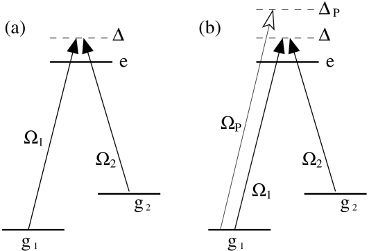
FIG. 1.: (a) Level Scheme: The solid arrows represent the lasers at Rabi frequencies $\Omega_{1}$, $\Omega_{2}$, that couple to the transitions $|g_{1}\rangle\to|e\rangle$, $|g_{2}\rangle\to|e\rangle$, respectively, and are detuned of $\Delta$ from atomic resonance. (b) Addition of a probe at Rabi frequency $\Omega_{\rm P}$ and detuning $\Delta_{\rm P}$, coupling $|g_{1}\rangle\to|e\rangle$.

A The dark resonance

An exemplary atomic level configuration where the effects of quantum interference manifest is the $\Lambda$-transition. It consists in two electronic transitions, formed by two stable or metastable states that we label $|g_{1}\rangle$, $|g_{2}\rangle$, which are coupled by lasers to the same excited state $|e\rangle$. For a closed transition, the atom stops to fluoresce when the states $|g_{1}\rangle$ and $|g_{2}\rangle$ are resonantly coupled (two-photon resonance), as shown in Fig. 1(a): The system evolves into the dark state, a stable atomic-states superposition which is decoupled from the excited state because of destructive interference between the excitation amplitudes. This phenomenon is called Coherent Population Trapping [7], and the atoms are found in the coherence (dark state)

$$|\Psi_{\rm D}\rangle=\frac{1}{\Omega}\left(\Omega_{2}|g_{1}\rangle-\Omega_{1}|g_{2}\rangle\right),$$ (1)

where $\Omega=\sqrt{\Omega_{1}^{2}+\Omega_{2}^{2}}$ and $\Omega_{1}$ ($\Omega_{2}$) is the Rabi frequency of the laser coupling to the transition $|g_{1}\rangle\to|e\rangle$ ($|g_{2}\rangle\to|e\rangle$). Here, without loss of generality we have assumed $\Omega_{1}$, $\Omega_{2}$ real. The dark state is accessed by spontaneous emission, unless the system has been initially prepared in it. Thus, the density matrix $\rho_{\rm D}=|\Psi_{\rm D}\rangle\langle\Psi_{\rm D}|$ is the steady-state solution of the master equation for the atomic density matrix $\rho$: $\partial\rho/\partial t={\cal L}_{0}\rho$, where ${\cal L}_{0}$ is the Liouvillian defined as

$${\cal L}_{0}\rho=\frac{1}{{\rm i}\hbar}[H,\rho]+{\cal K}\rho.$$ (2)

Here, $H=H_{0}+V_{0}$ is the Hamilton operator, and its terms have the form (in the rotating wave approximation and in the frame rotating at the laser frequencies)

$$H_{0} = -\hbar\Delta\left(|g_{1}\rangle\langle g_{1}|+|g_{2}\rangle\langle g_{2}|\right),$$ (3)

$$V_{0} = \frac{\hbar}{2}\left(\Omega_{1}|e\rangle\langle g_{1}|+\Omega_{2}|e\rangle\langle g_{2}|+{\rm H.c.}\right),$$ (4)

where $\Delta=\omega_{1}-\omega_{\rm L,1}=\omega_{2}-\omega_{\rm L,2}$ are the laser detunings, with the atomic resonance frequencies $\omega_{j}$ of the transition $|g_{j}\rangle\to|e\rangle$ and the frequencies of the corresponding driving laser $\omega_{{\rm L},j}$ ($j=1,2$). The operator ${\cal K}$ is the Liouvillian describing spontaneous emission,

$${\cal K}\rho=-\frac{\gamma}{2}\left[|e\rangle\langle e|\rho+\rho|e\rangle\langle e|\right]+\sum_{j=1,2}\gamma_{j}|g_{j}\rangle\langle e|\rho|e\rangle\langle g_{j}|,$$ (5)

where $\gamma_{1}$, $\gamma_{2}$ are the rate of decay into $|g_{1}\rangle$, $|g_{2}\rangle$, respectively, and $\gamma_{1}+\gamma_{2}=\gamma$. It can be easily verified that the dark state is a dressed state of the system, i.e. an eigenstate of $H$. The other two dressed states read [16]

$$|\psi_{+}\rangle=\cos\theta|e\rangle+\sin\theta|\psi_{\rm C}\rangle,$$ (6)

$$|\psi_{-}\rangle=\sin\theta|e\rangle-\cos\theta|\psi_{\rm C}\rangle,$$ (7)

where

$$\tan\theta=\frac{\sqrt{\Delta^{2}+\Omega^{2}}-\Delta}{\Omega},$$ (8)

$$|\psi_{\rm C}\rangle=\frac{1}{\Omega}\left(\Omega_{1}|g_{1}\rangle+\Omega_{2}|g_{2}\rangle\right),$$ (9)

and where we have introduced the state $|\psi_{\rm C}\rangle$, orthogonal to $|e\rangle$ and $|\psi_{\rm D}\rangle$. The states (6), (7) are at eigenfrequencies $\delta\omega_{\pm}=(\Delta\mp\sqrt{\Delta^{2}+\Omega^{2}})/2$, and since they possess non-zero overlap with the excited state $|e\rangle$, they have a finite decay rate and are populated in the transient dynamics. We denote their linewidths with $\gamma_{+}$, $\gamma_{-}$. The steady state is accessed at the slowest rate of decay and, for later convenience, we introduce $T_{0}$, the time scale corresponding to the inverse of this rate.
The dressed-state picture is a useful tool for interpreting the atomic spectra in a pump-probe experiment, where, e.g., a weak probe at Rabi frequency $\Omega_{\rm P}$ ($\Omega_{\rm P}\ll\Omega_{1},\Omega_{2}$) couples to the transition $|g_{1}\rangle\to|e\rangle$ as shown in Fig. 1(b), while its frequency is let sweep across the atomic resonance. Figure 2 shows the spectrum of excitation as a function of the detuning of the probe $\Delta_{\rm P}$, for a certain choice of the lasers parameters. Here, one can observe that the component of the spectrum at $\Delta_{\rm P}=\Delta$ is zero, corresponding to the situation where the system is in the dark state $|\Psi_{\rm D}\rangle$. Moreover, the spectrum exhibits two resonances centered at $\Delta_{\rm P}=\delta\omega_{\pm}$, whose widths correspond approximately (when $|\Delta|,\Omega\gg\gamma$) to $\gamma_{+}$, $\gamma_{-}$, respectively, and can be identified with the dressed states $|\psi_{+}\rangle$, $|\psi_{-}\rangle$ [17]. Note that these resonance have not a Lorentzian shape: The spectrum shares in fact many similarities with a Fano profile [17]. Typical excitation spectra, measured with a single ion in a trap, are reported in [18, 19].

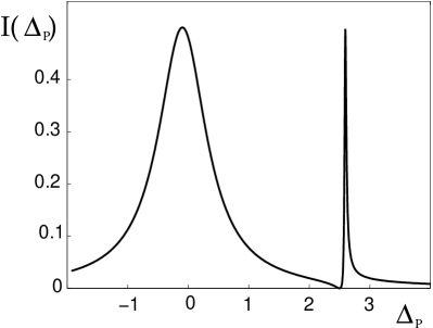
FIG. 2.: Excitation spectrum $I(\Delta_{\rm P})$ in arbitrary units as a function of the probe detuning $\Delta_{\rm P}$ in unit of $\gamma$. Here, $\Omega=\gamma$, $\Delta=2.5\gamma$ $\Omega_{\rm P}=0.05\gamma$.

B The motion

We consider now the center-of-mass motion in presence of a conservative potential, of which for the moment the form is not specified. Given the mass of the atom $m$, the momentum $p$, the position $x$ and the potential $U(x)$, the mechanical Hamiltonian is

$$H_{\rm mec}=\frac{p^{2}}{2m}+U(x).$$ (10)

We denote with $|\psi_{\epsilon}\rangle$ the eigenvectors of $H_{\rm mec}$ at the eigenvalues $\epsilon$. The full dynamics are now described by the Master equation

$$\frac{\partial}{\partial t}\tilde{\rho}=\frac{1}{{\rm i}\hbar}[\tilde{H},\tilde{\rho}]+\tilde{\cal K}\tilde{\rho}=\tilde{\cal L}\tilde{\rho},$$ (11)

where $\tilde{\rho}$ is the density matrix for the internal and external degrees of freedom and

$$\tilde{H}=\tilde{H}_{0}+H_{\rm mec}+\tilde{V}.$$ (12)

Here, $\tilde{V}$ describes the coherent interaction of the atomic dipole with the lasers, and has the form

$$\tilde{V}=\frac{\hbar}{2}\left(\Omega_{1}{\rm e}^{{\rm i}k_{1}x\cos\phi_{1}}|e\rangle\langle g_{1}|+\Omega_{2}{\rm e}^{{\rm i}k_{2}x\cos\phi_{2}}|e\rangle\langle g_{2}|+{\rm H.c.}\right),$$ (13)

where the lasers are travelling waves at wave vectors $k_{1}$ and $k_{2}$, propagating along the directions forming the angles $\phi_{1}$, $\phi_{2}$, respectively, with the $\hat{x}$-axis. In (13) the spatial dependence is explicitly included, which couples to the external degrees of freedom of the ion, while the Rabi frequencies $\Omega_{1}$, $\Omega_{2}$ are assumed to be constant over the spatial region where the ion is localized. The liouvillian $\tilde{\cal K}$ describes the incoherent scattering processes, whereby a photon is spontaneously emitted under an angle $\phi$ with the axis of the motion. It has the form:

$$\tilde{\cal K}\tilde{\rho}= - \frac{\gamma}{2}\left[|e\rangle\langle e|\tilde{\rho}+\tilde{\rho}|e\rangle\langle e|\right]$$ (14)

$$+ \sum_{j=1,2}\gamma_{j}\int_{-1}^{1}{\rm d}\cos\phi{\cal N}(\cos\phi)|g_{j}\rangle\langle e|\left[{\rm e}^{{\rm i}k_{j}x\cos\phi}\tilde{\rho}{\rm e}^{-{\rm i}k_{j}x\cos\phi}\right]|e\rangle\langle g_{j}|,$$ (15)

where ${\cal N}(\cos\phi)$ is the probability distribution for the angles of photon emission respect to the motional axis.
In this system, at a given instant of time perfect destructive interference between excitation amplitudes occurs for the state

$$|\tilde{\Psi}_{\rm D}\rangle=\frac{1}{\Omega}\left(\Omega_{2}|g_{1},\Psi\rangle-\Omega_{1}{\rm e}^{{\rm i}(k_{1}\cos\phi_{1}-k_{2}\cos\phi_{2})x}|g_{2},\Psi\rangle\right),$$ (16)

where $\exp({\rm i}(k_{1}\cos\phi_{1}-k_{2}\cos\phi_{2})x)$ is the displacement operator, acting on the external degrees of freedom, and $\Psi$ is a state of the center-of-mass motion. The state (16) is stable -and thus a dark state- if it is eigenstate of $H_{0}+H_{\rm mec}$. This is always true when the lasers are copropagating and $k_{1}\cos\phi_{1}=k_{2}\cos\phi_{2}$ (or, for one-dimensional motion as in this case, when the direction of propagation of the lasers is orthogonal to the axis of the motion, $\cos\phi_{1}=\cos\phi_{2}=0$): Then, the motional state factorizes out in (16). For $k_{1}\cos\phi_{1}\neq k_{2}\cos\phi_{2}$, on the contrary, one must consider the particular form of the confining potential. For instance, for free atoms ($U(x)=$ const.) a perfect dark state exists for $k_{1}\cos\phi_{1}=-k_{2}\cos\phi_{2}=k$ and reads $|\tilde{\Psi}_{\rm D}\rangle=\left(\Omega_{2}|g_{1},-\hbar k\rangle-\Omega_{1}|g_{2},\hbar k\rangle\right)/\Omega$. This property has been used to prepare very cold atomic samples [20]. In presence of a confining potential, on the other hand, there exists in general no state $|\tilde{\Psi}_{\rm D}\rangle$ that is perfectly dark. Approximate dark states have been discussed in [15] for a 1D flat-bottom and for a 2D harmonic trap.

Nevertheless, transient CPT can be observed in trapping potentials and in Doppler-sensitive configurations when the atoms are in the Lamb-Dicke regime (LDR), i.e. when the size of their motional wave packet $\sqrt{\langle\Delta x^{2}\rangle}$ is much smaller than the wavelength of the light, $k_{1,2}\sqrt{\langle\Delta x^{2}\rangle}\ll 1$. In this limit, a hierarchy of processes in the excitation of the center-of-mass wave packet is estabilished. At zero order in $\zeta=k_{1,2}\sqrt{\langle\Delta x^{2}\rangle}$, the effects due to the spatial gradient of the light-atom potential are neglected: the atoms behave like they were point-like, and the coherent transitions take place at the laser frequency (carrier). Then, after the transient time $T_{0}$ the atoms have accessed the internal dark state $|\Psi_{\rm D}\rangle$. At first order in $\zeta$, effects due to the finite size of the motional wave-packet become manifest, and transitions between different motional states (sidebands transitions) occur. On this longer time scale, that we denote with $T_{\zeta}$, the atom is optically pumped out of the dark state into another state of the motion. In the Lamb-Dicke regime, the relation $T_{\zeta}\gg T_{0}$ allows for a coarse-grained description of the dynamics, where the internal state of the atom is assumed to be always the dark state $|\Psi_{\rm D}\rangle$.
These arguments suggest that for a trapped atom in the LDR some of the properties of the excitation spectrum discussed for the Doppler-free case may also be applicable to the Doppler-sensitive one. Here, the carrier transition is predominant, whereas transitions which change the state of the motion (sidebands transitions) are of higher order in the Lamb-Dicke parameter, and can be interpreted as transitions due to a probe ($\Omega_{\rm P}$) set at the corresponding frequency in the bare atom, as illustrated for instance in Fig. 1(b). In the next section, we show that this interpretation is theoretically justified.

III Theory

Here, we derive the equations for the center-of-mass motion in the limit where the LDR applies and when the center-of-mass motion is confined by the same potential at all three electronic levels. The procedure consists in adiabatically eliminating the internal degrees of freedom from the dynamical equation at second order in the parameter $\zeta$, and it corresponds to analysing the coarse-grained evolution on the time interval $\Delta t$ such that $T_{\zeta}\gg\Delta t\gg T_{0}$. The formalism we use has been first developed in [11] for a two-level transition driven by a running wave, and later applied to standing-wave drives and multilevel transitions in [21]. In the following, we outline the fundamental steps that are most general to all treatments, and refer the reader to [11, 21] for details (we have used the same notation as in [21] when possible).

1 Lamb-Dicke limit

In the Lamb-Dicke limit $\zeta\ll 1$, the operators $\exp({\rm i}k_{j}x)$ appearing in (13),(14) can be expanded in powers of $\zeta$. At second order in this expansion Eq. (11) can be rewritten as

$$\frac{\partial}{\partial t}\tilde{\rho}=\left[\tilde{\cal L}_{0}+\tilde{\cal L}_{1}+\tilde{\cal L}_{2}\right]\tilde{\rho},$$ (17)

where the Liouvillians $\tilde{\cal L}_{j}$ describe processes at the $j$th order in the Lamb-Dicke parameter, and are defined as:

$$\tilde{\cal L}_{0}\tilde{\rho} = {\cal L}_{0}\tilde{\rho}+\frac{1}{{\rm i}\hbar}[H_{\rm mec},\tilde{\rho}],$$ (18)

$$\tilde{\cal L}_{1}\tilde{\rho} = \frac{1}{{\rm i}\hbar}[xV_{1},\tilde{\rho}],$$ (19)

$$\tilde{\cal L}_{2}\tilde{\rho} = \frac{1}{{\rm i}\hbar}[x^{2}V_{2},\tilde{\rho}]+\tilde{\cal K}_{2}\tilde{\rho}.$$ (20)

Here, $V_{1}$, $V_{2}$ are the first and second order terms in the expansion of $\tilde{V}$ and read

$$V_{1} = \frac{{\rm i}\hbar}{2}\sum_{j=1,2}k_{j}\cos\phi_{j}\Omega_{j}\left(|e\rangle\langle g_{j}|-|g_{j}\rangle\langle e|\right),$$ (21)

$$V_{2} = -\frac{\hbar}{4}\sum_{j=1,2}k_{j}^{2}\cos^{2}\phi_{j}\Omega_{j}\left(|e\rangle\langle g_{j}|+|g_{j}\rangle\langle e|\right).$$ (22)

The Liouvillian $\tilde{\cal K}_{2}$ has the form:

$$\tilde{\cal K}_{2}\tilde{\rho}=\alpha\sum_{j=1,2}\gamma_{j}k_{j}^{2}|g_{j}\rangle\langle e|\left(2x\tilde{\rho}x-x^{2}\tilde{\rho}-\tilde{\rho}x^{2}\right)|e\rangle\langle g_{j}|,$$ (23)

where $\alpha=\int_{-1}^{1}{\rm d}\cos\phi{\cal N}(\cos\phi)\cos^{2}\phi$.

At zero order in $\zeta$, internal and external degrees of freedom are decoupled: The state $\tilde{\rho}_{\rm St}$, solution of $\tilde{\cal L}_{0}\tilde{\rho}=0$, is not uniquely defined, and has the form $\tilde{\rho}_{\rm St}=\rho_{\rm St}\otimes\mu(0)$, where $\rho_{\rm St}=\rho_{\rm D}$ is the internal steady state and $\mu(0)={\rm Tr}_{\rm int}\{{\cal P}_{0}\tilde{\rho}(0)\}$ is the reduced density matrix, calculated from $\tilde{\rho}$ at $t=0$ by tracing over the internal degrees of freedom (${\rm Tr}_{\rm int}\{\}$) and applying the projector ${\cal P}_{0}$ acting over the external degrees of freedom. The latter is defined as ${\cal P}_{0}\tilde{\rho}=\sum_{\epsilon}\sum_{\psi_{\epsilon},\psi_{\epsilon}^{\prime}}^{\prime}|\psi_{\epsilon}\rangle\langle\psi_{\epsilon}^{\prime}|\langle\psi_{\epsilon}|\tilde{\rho}|\psi_{\epsilon}^{\prime}\rangle$, where $|\psi_{\epsilon}\rangle$, $|\psi_{\epsilon}^{\prime}\rangle$ are eigenstates of $H_{\rm mec}$ at $\epsilon$. In general, at zero order equation $\partial_{t}\tilde{\rho}=\tilde{\cal L}_{0}\tilde{\rho}$ admits an infinite number of stable solutions. They can be expanded in the basis of (left) eigenvectors $\tilde{\rho}_{\epsilon,\epsilon^{\prime}}=\rho_{\rm St}\otimes|\psi_{\epsilon}\rangle\langle\psi_{\epsilon^{\prime}}|$ at the (imaginary) eigenvalues $\lambda_{\epsilon,\epsilon^{\prime}}=-{\rm i}(\epsilon-\epsilon^{\prime})/\hbar$ of the Liouville operator $\tilde{\cal L}_{0}$, satisfying the secular equation $\tilde{\cal L}_{0}\tilde{\rho}_{\epsilon,\epsilon^{\prime}}=\lambda_{\epsilon,\epsilon^{\prime}}\tilde{\rho}_{\epsilon,\epsilon^{\prime}}$ ($\tilde{\rho}_{\rm St}$ is eigenvector at $\lambda=0$). The eigenspaces at the eigenvalues $\lambda_{\epsilon,\epsilon^{\prime}}$ may be also infinitely degenerate, as it occurs for instance in the harmonic oscillator. For $\zeta\neq 0$ these subspaces are coupled by $\tilde{\cal L}_{1}$, $\tilde{\cal L}_{2}$. At second-order perturbation theory in $\zeta$, for $\zeta_{j}\Omega_{j}\ll\min_{\epsilon,\epsilon^{\prime}\neq\epsilon}\left(|\epsilon-\epsilon^{\prime}|\right)$ (i.e. when the spectum of $\tilde{\cal L}_{0}$ is sufficiently spaced, to allow for non-degenerate perturbation theory), a closed equation for the dynamics in the subspace at $\lambda=0$ can be derived. Denoting with $\tilde{\cal P}_{0}$ the projector onto this subspace, defined as $\tilde{\cal P}_{0}\tilde{\rho}=\rho_{\rm St}\otimes{\rm Tr}_{\rm int}\{{\cal P}_{0}\tilde{\rho}\}$, this equation has the form [11]:

$$\frac{\rm d}{{\rm d}t}\tilde{\cal P}_{0}\tilde{\rho}(t)=\left[\tilde{\cal P}_{0}\tilde{\cal L}_{2}\tilde{\cal P}_{0}+\int_{0}^{\infty}{\rm d}\tau\tilde{\cal P}_{0}\tilde{\cal L}_{1}{\rm e}^{\tilde{\cal L}_{0}\tau}\tilde{\cal L}_{1}\tilde{\cal P}_{0}\right]\tilde{\rho}(t).$$ (24)

After substituting the explicit form of $\tilde{\cal L}_{1},\tilde{\cal L}_{2}$ in the second term on the right-hand side of (24) and tracing over the internal degrees of freedom, we obtain:

$$\frac{\rm d}{{\rm d}t}\mu = -{\cal P}_{0}\frac{1}{\hbar^{2}}\int_{0}^{\infty}{\rm d}\tau\Bigl{(}\mbox{Tr}_{\rm int}\left\{V_{1}{\rm e}^{{\cal L}_{0}\tau}V_{1}\rho_{\rm St}\right\}[\hat{x},[\hat{x}(\tau),\mu]]$$ (25)

$$+ \mbox{Tr}_{\rm int}\left\{V_{1}{\rm e}^{{\cal L}_{0}\tau}[V_{1},\rho_{\rm St}]\right\}[\hat{x},\mu\hat{x}(\tau)]\Bigr{)}.$$ (26)

Here, the matrix $\mu={\rm Tr}_{\rm int}\{{\cal P}_{0}\tilde{\rho}\}$ is the reduced density matrix for the external degrees of freedom in the subspace at eigenvalue (at zero order) $\lambda=0$. The operator $\hat{x}(\tau)$ is here defined as $\hat{x}(\tau)=\exp(-{\rm i}H_{\rm mec}\tau/\hbar)\hat{x}\exp({\rm i}H_{\rm mec}\tau/\hbar)$.

It is remarkable that the term $\tilde{\cal P}_{0}\tilde{\cal L}_{2}\tilde{\cal P}_{0}=0$. This result is explained by looking at the form of (20). When tracing over the internal degrees of freedom, the first term of (20) gives rise to a contribution proportional to ${\rm Tr}_{\rm int}\{V_{2}\rho_{\rm St}\}$: This term usually gives rise to a shift to the eigenvalues $\lambda_{\epsilon,\epsilon^{\prime}}$, it represents a renormalization of the harmonic oscillator frequency due to the presence of the laser fields, and here it vanishes since there is no occupation of the excited state at steady state. The second term in (20) describes the diffusion arising from spontaneous emission into other mechanical states [21]. Again, since at steady state there is no excited-state occupation, it vanishes. Thus, the disapperance of $\tilde{\cal P}_{0}\tilde{\cal L}_{2}\tilde{\cal P}_{0}$ is due to quantum interference at zero order in the Lamb-Dicke expansion.

For a non-degenerate spectrum of eigenvalues $\epsilon$, the reduced matrix $\mu$ is diagonal, and the equation for a matrix element has the form

$$\frac{\rm d}{{\rm d}t}\langle\psi_{\epsilon}|\mu|\psi_{\epsilon}\rangle=\sum_{\epsilon^{\prime}}C_{\epsilon,\epsilon^{\prime}}S(\omega_{\epsilon,\epsilon^{\prime}})\left[-\langle\psi_{\epsilon}|\mu|\psi_{\epsilon}\rangle+\langle\psi_{\epsilon^{\prime}}|\mu|\psi_{\epsilon^{\prime}}\rangle\right]+{\rm H.c},$$ (27)

where the coefficient $S(\omega_{\epsilon,\epsilon^{\prime}})$ is the value of fluctuation spectrum of the operator $V_{1}$ at the frequency ${\omega_{\epsilon,\epsilon^{\prime}}=\left[\epsilon-\epsilon^{\prime}\right]/\hbar}$, and reads

$$S(\omega_{\epsilon,\epsilon^{\prime}})=\frac{1}{\hbar^{2}}\int_{0}^{\infty}{\rm d}\tau{\rm Tr}_{\rm int}\left\{V_{1}{\rm e}^{{\cal L}_{0}\tau}V_{1}\rho_{\rm St}\right\}{\rm e}^{{\rm i}(\epsilon-\epsilon^{\prime})\tau/\hbar}.$$ (28)

The coefficient $C_{\epsilon,\epsilon^{\prime}}=|\langle\psi_{\epsilon}|x|\psi_{\epsilon^{\prime}}\rangle|^{2}$ weights the coupling between the center-of-mass states $|\psi_{\epsilon}\rangle$ and $|\psi_{\epsilon^{\prime}}\rangle$ due to the photon momentum at second order in the Lamb-Dicke expansion. The equations necessary for the derivation of the explicit form of (28) are reported in appendix A. Equation (28) shows that the rate for the transition $|\psi_{\epsilon}\rangle\to|\psi_{\epsilon^{\prime}}\rangle$ is given by the value of the excitation spectrum for a probe, whose interaction with the atomic transition is described by $V_{1}$ and which is detuned from the pump by $\omega_{\epsilon,\epsilon^{\prime}}$ (sideband transition). Here, the form of the potential enters explicitly through the coefficients $C_{\epsilon,\epsilon^{\prime}}$, and implicitly through the assumptions on the spectrum that have lead to (27).

A Harmonic oscillator

We now let the potential be harmonic at frequency $\nu$, $U(x)=\frac{1}{2}m\nu^{2}x^{2}$, and introduce the annihilation and creation operators $a$ and $a^{\dagger}$ of a quantum of vibrational energy $\hbar\nu$, such that $x=x_{0}(a^{\dagger}+a)$, $p={\rm i}p_{0}(a^{\dagger}-a)$, with $x_{0}=\sqrt{\hbar/2m\nu}$ and $p_{0}=\sqrt{\hbar m\nu/2}$. The center-of-mass Hamiltonian reads

$$H_{\rm mec}=\hbar\nu\left(a^{\dagger}a+\frac{1}{2}\right).$$ (29)

Now, $|\psi_{\epsilon}\rangle=|n\rangle$ and $\epsilon=\hbar\nu(n+1/2)$, where $n=0,1,\ldots$ is the number of phonon excitations, and the mechanical energies are equidistantly spaced by $\hbar\nu$. The coefficients $C_{n,n^{\prime}}=x_{0}^{2}(n\delta_{n^{\prime},n-1}+(n+1)\delta_{n^{\prime},n+1})$, and thus at first order in the Lamb-Dicke expansion the relevant transitions between motional states are the blue sideband $|n\rangle\to|n+1\rangle$ at frequency $\omega_{L}-\nu$, and the red sideband $|n\rangle\to|n-1\rangle$ at frequency $\omega_{L}+\nu$. We define the Lamb-Dicke parameter $\eta_{j}=k_{j}x_{0}$, that fulfills the relation $\zeta_{1,2}=\eta_{1,2}\sqrt{2\langle n\rangle+1}$, with $\langle n\rangle$ average number of phonon excitations.
For the harmonic oscillator the equations derived in the previous section simplify notably: Equation (26) gets the form

$$\frac{\rm d}{{\rm d}t}\mu = x_{0}^{2}S(\nu)\left[-a^{\dagger}a\mu+a\mu a^{\dagger}\right]$$ (30)

$$+ x_{0}^{2}S(-\nu)\left[-aa^{\dagger}\mu+a^{\dagger}\mu a\right]+{\rm H.c},$$ (31)

and for the probability $\mu_{n,n}=\langle n|\mu|n\rangle$ of the system to be in the number state $|n\rangle$, Eq. (30) turns to a rate equation, whose form is well known in laser cooling of single ions [23],

$$\frac{\rm d}{{\rm d}t}\mu_{n,n} = \eta^{2}[(n+1)(A_{-}\mu_{n+1,n+1}-A_{+}\mu_{n,n})$$ (33)

$$+n(A_{-}\mu_{n,n}-A_{+}\mu_{n-1,n-1})].$$

In our case of a three-level atom, $\eta=\eta_{1}\cos\phi_{1}-\eta_{2}\cos\phi_{2}$, and

$$A_{\pm}=2\mbox{Re}[S(\mp\nu)]=\frac{1}{4}\left(\frac{\Omega_{1}\Omega_{2}}{\Omega}\right)^{2}\frac{\gamma\nu^{2}}{\left[\Omega^{2}/4-\nu(\nu\pm\Delta)\right]^{2}+\gamma^{2}\nu^{2}/4}.$$ (34)

Equation (33) has the same structure as the rate equation derived for sideband cooling in a two-level system. Here, however, the rates $A_{\pm}$ describe the sideband excitation including the effect of quantum interference between the atomic transitions. Equation (33) allows for a steady state when $A_{-}>A_{+}$, which is fulfilled when $\Delta<0$ (blue detuning) and $\Omega>2\nu$, or when $\Delta>0$ (red detuning) and $\Omega<2\nu$. The value of the trap frequency $\bar{\nu}=\Omega/2$ separates two regimes: for $\nu<\Omega/2$ it is the narrow resonance that determines relevantly the center-of-mass dynamics, whereas for $\nu>\Omega/2$ the sideband transitions are at the frequency range of the broad resonance [22]. We remark that $\eta=0$ for $k_{1}\cos\phi_{1}=k_{2}\cos\phi_{2}$, corresponding to the Doppler-free situation. Furthermore, the Lamb-Dicke parameter entering into the dynamics is the one determined by the laser wave vector. The Lamb-Dicke parameter connected to spontaneous emission events (i.e. recoils because of emission into other states of the motion) does not appear, since the diffusion term vanishes at second order in the Lamb-Dicke expansion.
In the following we assume $k_{1}\cos\phi_{1}\neq k_{2}\cos\phi_{2}$ and $\Delta<0$, $\Omega>2\nu$ ($A_{-}>A_{+}$). Insight into the dynamics can be gained from the equation for the average number of phonon $\langle n(t)\rangle=\sum_{n=0}^{\infty}n\mu_{n,n}(t)$, that is derived from (33) and has the form [23]

$$\frac{\rm d}{{\rm d}t}\langle n\rangle=-W\langle n\rangle+\eta^{2}A_{+},$$ (35)

where $W=\eta^{2}(A_{-}-A_{+})$ is the cooling rate. The steady state value $\langle n\rangle_{\infty}$ reads

$$\langle n\rangle_{\infty}=\frac{4\left[\Omega^{2}/4-\nu(\nu-\Delta)\right]^{2}+\gamma^{2}\nu^{2}}{4\nu|\Delta|(\Omega^{2}-4\nu^{2})},$$ (36)

and is minimum when $\Omega^{2}=4\nu(\nu-\Delta)$. This relation corresponds to setting the a.c. Stark shift $\delta\omega_{+}$ of the narrow resonance $|\Psi_{+}\rangle$ at the frequency of the first red sideband, $\delta\omega_{+}=\Delta-\nu$. For this value, $\langle n\rangle_{\infty}^{({\rm min})}=(\gamma/4|\Delta|)^{2}$: Hence, low temperatures are achieved for lasers far detuned from atomic resonance. This corresponds to an enhanced asymmetry of the excitation spectrum, as the one shown in Fig. 2, where the two resonances have very different widths.

For $\delta\omega_{+}=\Delta-\nu$ the cooling rate scales as

$$W^{\rm max}\sim\eta^{2}(\Omega_{1}\Omega_{2}/\Omega)^{2}/\gamma.$$ (37)

Thus, fast cooling is achieved for large Rabi frequencies and when $\Omega_{1}=\Omega_{2}$. The ultimate limit to $W$ is set by the parameters that ensure the validity of the perturbative treatment here applied: This is valid for $\eta_{j}\Omega_{j}\cos\theta\ll\gamma_{+}$ ($j=1,2$), with $\gamma_{+}\sim\gamma\cos^{2}\theta$ linewidth of the narrow resonance, corresponding in the bare atom to the situation where the probe (the sideband) does not saturate the transition to $|\Psi_{+}\rangle$. At $\delta\omega_{+}=\Delta-\nu$, one has $\gamma_{+}\sim\nu\gamma/4\sqrt{\Delta^{2}+\Omega^{2}}$, which sets the fastest rate at which efficient laser cooling can occur, $W^{\rm max}\sim\gamma_{+}/2$.

It is remarkable that these results do not depend on the branching ratio $\gamma_{1}/\gamma_{2}$. In fact, in this limit the branching ratio enters the problem only through $T_{0}$. Nevertheless, a too large branching ratio affects the time scale $T_{0}$ at which the transient steady-state is reached.

In Fig. 3 we test the validity of the adiabatic elimination procedure for various values of the Lamb-Dicke parameter, by comparing the results predicted by (35) with a full numerical simulation. The parameters are reported in the caption. Full agreement between the two results is found for $\eta=0.02$ ($\eta_{1}\cos\phi_{1}=-\eta_{2}\cos\phi_{2}=0.01$). It should be mentioned that in [6] full agreement has been found for $\eta$ as large as 0.2. On the other hand, those results have been evaluated for the case $\Omega_{1}\ll\Omega_{2}$, and the small value of $\Omega_{1}$ ensured the validity of the perturbative expansion.

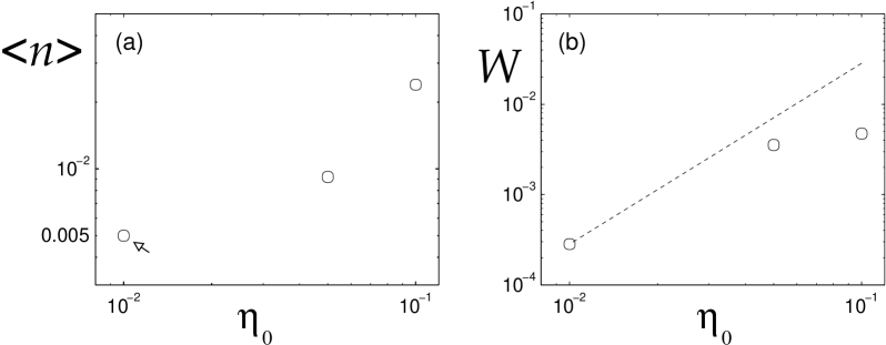
FIG. 3.: Plot of (a) $\langle n\rangle_{\infty}$ and (b) $W$ as a function of $\eta_{0}$. Dashed line: rate equation result; ’o’: numerical simulation, 500 trajectories with the Quantum Monte Carlo method. Here, $\eta_{1}\cos\phi_{1}=\eta_{2}\cos\phi_{2}=\eta_{0}$ ($\eta=2\eta_{0}$), $\nu=2$ MHz, $\gamma=20$ MHz, $\Omega_{1}=\Omega_{2}=17$ MHz, $\Delta=70$ MHz, $\gamma_{1}/\gamma_{2}=1$. In (a) the result of the simulation in agreement with the rate equation prediction ($\langle n\rangle=0.005$) is indicated by the arrow. In (b) the rate $W$ is in units of $\gamma/2$.

1 Discussion

We have shown that, by properly choosing the lasers parameters, one can achieve almost unity ground-state occupation with this cooling method (EIT cooling). The state $|\psi_{\rm D}\rangle|0\rangle$ is equivalent to the ground state in sideband cooling, since it is only off-resonantly (weakly) coupled to other states, and it satisfies the criteria of an approximate dark state as discussed in [15].

From (34) one recovers the rates of Eq. (4) in [6] in the limit $\Omega_{1}\ll\Omega_{2}$. We have shown that the same dynamics are encountered in more general situations, that do not impose a specific relation between the two Rabi frequencies. From the technical point of view EIT cooling proves again to be more advantageous than Raman sideband cooling (see [6, 9]). Such advantage is mainly twofold. On one hand, in EIT cooling both lasers cool the atom, and a decay into one or the other channel does not affect the efficiency of the process, while in Raman sideband cooling a finite branching ratio gives rise to heating [24]. Another important feature of EIT cooling is the disappearance of the carrier absorption due to quantum interference. This effect implies the suppression of diffusive processes: Since in the coarse-grained evolution the excited state is effectively empty, processes, where the atom is scattered into other motional states by spontaneous emission, disappear at second order in the Lamb-Dicke expansion. That implies an improved efficiency with respect to Raman-sideband cooling, where instead such processes are present, as already discussed in [6].

It is instructive to compare the dynamics in EIT cooling with the dynamics of a trapped ion at the node of a standing wave, as studied for example in [21]. At the node of a standing wave the carrier absorption cancels, since here the value of the electric field is zero. Nevertheless, sideband absorption occurs because of the finite size of the motional wave packet. In the case of a $\Lambda$- configuration driven by two travelling waves at two-photon resonance, the transient dark state (16) is a superposition of the states $|g_{1}\rangle$ and $|g_{2}\rangle$ whose relative phase is a function of the coordinate $x$, so that the finite size of the wave packet allows sideband absorption also in this case. Nevertheless, in the LDR the gradient of the phase over the wavepacket is small, and the sideband transitions are excited on a longer time scale. This can be illustrated when writing the atom-laser interaction (13) at the first order in the Lamb-Dicke expansion and in the form

$$\tilde{V}\approx\hbar\frac{\Omega}{2}\left[|e\rangle\langle\Psi_{\rm C}|+{\rm i}|e\rangle\langle\Psi_{\rm D}|kx+{\rm H.c.}\right],$$ (38)

where we have made the simplifying assumptions $\Omega_{1}=\Omega_{2}=\Omega/\sqrt{2}$, $k_{1}\cos\phi_{1}=-k_{2}\cos\phi_{2}=k$. Here, we see that the dark state is coupled to the excited state at first order in the Lamb-Dicke expansion, for effects arising from the finite size of the motional wave packet.

The atom dynamics during the coarse-grained evolution can be interpreted in terms of field gradients over the size of the wave-packet, that give rise to forces [25]. In this respect, one can say that this method uses the phase gradient of the dark state, due to the spatial gradient of the total field, for achieving cooling. In this context, we remark that the operator $V_{1}$ in (28) is the gradient of the potential (13) at $x=0$, i.e. at the center of trap.

Finally, we apply the results obtained for the harmonic oscillator to the case of a generic potential $U(x)$. Several conclusions drawn in this section are applicable to the case described in Eq. (27), when the mechanical Hamiltonian has a discrete spectrum, and the minimum distance between two neighbouring energy level is sufficiently large to allow for non-degenerate perturbation theory. Laser cooling is here achieved for the same parameters as for the harmonic oscillator. However, the narrow resonance enhances transitions in a finite range of frequencies ($<\bar{\nu}$), and $\delta\omega_{+}$ must be properly tuned, e.g. to the average value of the red sideband transitions frequencies. The process will thus be efficient under the condition that, for each motional state, there is a sufficient number of red sidebands inside this range, so that the rate of cooling for a given motional state is larger than the rate of heating.

An interesting question is how the dynamics are affected when the external potential depends on the electronic state, and thus when

$$U(x)=U_{1}(x)|g_{1}\rangle\langle g_{1}|+U_{e}(x)|e\rangle\langle e|+U_{2}(x)|g_{2}\rangle\langle g_{2}|.$$

We consider first the case $U_{1}(x)=U_{2}(x)$, while $U_{e}(x)$ is -say- constant, so that the center of mass of the excited atom is not spatially confined and the spectrum of $H_{\rm mec}$ at the state $|e\rangle$ is a continuum. Assuming that for $U_{1}$, $U_{2}$ the Lamb-Dicke regime holds, then at two-photon resonance and during the transient dynamics the atom is optically pumped into the (transient) dark state (1). However, during $T_{0}$ the center-of-mass wave packet changes, since each eigestate of $U_{1}(x)$ ($U_{2}(x)$) may have non-zero overlap with several eigenstates of $U_{e}(x)$. This effect constitutes a diffusion mechanism, that lowers the cooling efficiency and, outside of some regimes, can make it even impossible. Formally, for $U_{e}\neq U_{1},U_{2}$, the formalism applied in this section is not applicable, since one cannot separate the time scales characterizing the evolution of the internal and external degrees of freedom.
In the general case of three different confining potentials the presence of a dark state cannot be excluded: that however depends on the specific form of the functions $U_{j}(x)$.

IV Conclusions and outlook

We have presented a systematic investigation of the center-of-mass dynamics of a trapped ion, the internal transitions of which are driven by lasers in a $\Lambda$-type configuration and set at two-photon resonance. Assuming that the center-of-mass wavepacket is well localized over the laser wavelength (Lamb-Dicke regime), we have adiabatically eliminated the internal degrees of freedom from the equation of the center-of-mass dynamics, and obtained a set of rate equations for the occupation of the motional states. We have identified the parameter regimes where efficient ground-state cooling can be achieved. The derivation here presented provides the theoretical background for the equations in [6, 8, 9] and extends the parameter regime to cases which have not been previously considered. As also discussed in [6], we have shown that diffusive processes, encountered in cooling with two-level atoms or with effective two-level systems (Raman sideband cooling), are suppressed because of quantum interference between the dipole transitions at zero order in the Lamb-Dicke expansion. Cooling takes place because of excitations due to the spatial gradient of the electric field over the width of the motional wave-packet, that are due to the finite size of the wave-packet itself and occur at first order in the Lamb-Dicke expansion. The motion can be said to be cooled by both lasers, while the branching ratio does not affect in general the efficiency of the process.
Finally, we have discussed the possibility to observe these dynamics for other types of potentials, that may depend on the electronic state.

This work opens interesting prospects in the manipulation of the quantum center-of-mass motion of atoms by using quantum interference in driven multilevel transitions, that is subject of on-going investigations.

V Acknowledgements

The author ackowledges Jürgen Eschner, who has encouraged and stimulated the completion of this work with several discussions and critical comments. He is also ackowledged for the critical reading of this manuscript. Most part of this work has been done at the Max-Planck-Institut für Quantenoptik: the author is grateful to Herbert Walther for his support, and to the whole group in Garching for the enjoyable and stimulating scientific atmosphere. The author thanks Markus Cirone for the corrections to the english.

A Calculation of $S(\nu)$

The term $S(\nu)$ in (28) is the Laplace transform at ${\rm i}\nu$ of the correlation function $G(\tau)$, defined as $G(\tau)={\rm Tr}_{\rm int}\{V_{1}(\tau)V_{1}(0)\rho_{\rm St}\}$, where $V_{1}(\tau)=V_{1}{\rm e}^{{\cal L}_{0}\tau}$. This is evaluated applying the quantum regression theorem [16, 26]. In the following, we derive the equations that are essential for this calculation. For convenience, we introduce the vector-operator $\hat{\sigma}$ whose components are defined as: $\hat{\sigma}_{1}=|g_{1}\rangle\langle g_{1}|$, $\hat{\sigma}_{2}=|g_{2}\rangle\langle g_{2}|$, $\hat{\sigma}_{3}=|g_{1}\rangle\langle e|$, $\hat{\sigma}_{4}=|e\rangle\langle g_{1}|$, $\hat{\sigma}_{5}=|g_{2}\rangle\langle e|$, $\hat{\sigma}_{6}=|e\rangle\langle g_{2}|$, $\hat{\sigma}_{7}=|g_{2}\rangle\langle g_{1}|$, $\hat{\sigma}_{8}=|g_{1}\rangle\langle g_{2}|$. The mean value $\langle\hat{\sigma}_{j}\rangle={\rm Tr}\{\hat{\sigma}_{j}\rho\}$ obeys the equations ${\rm d}\langle\hat{\sigma}_{j}\rangle/{\rm d}t=M\langle\hat{\sigma}_{j}\rangle+B$, where $M$, $B$ are a matrix and a column vector, respectively, and are defined through the equations

$$\sum_{j=1}^{8}M_{1,j}\langle\hat{\sigma}_{j}\rangle=-\gamma_{1}(\langle\hat{\sigma}_{1}\rangle+\langle\hat{\sigma}_{2}\rangle)-{\rm i}\frac{\Omega_{1}}{2}\left(\langle\hat{\sigma}_{3}\rangle-\langle\hat{\sigma}_{4}\rangle\right),$$ (A1)

$$\sum_{j=1}^{8}M_{2,j}\langle\hat{\sigma}_{j}\rangle=-\gamma_{2}(\langle\hat{\sigma}_{1}\rangle+\langle\hat{\sigma}_{2}\rangle)-{\rm i}\frac{\Omega_{2}}{2}\left(\langle\hat{\sigma}_{5}\rangle-\langle\hat{\sigma}_{6}\rangle\right),$$ (A2)

$$\sum_{j=1}^{8}M_{3,j}\langle\hat{\sigma}_{j}\rangle=-{\rm i}\frac{\Omega_{1}}{2}\left(2\langle\hat{\sigma}_{1}\rangle+\langle\hat{\sigma}_{2}\rangle\right)-\left(\frac{\gamma}{2}+{\rm i}\Delta\right)\langle\hat{\sigma}_{3}\rangle-{\rm i}\frac{\Omega_{2}}{2}\langle\hat{\sigma}_{8}\rangle,$$ (A3)

$$\sum_{j=1}^{8}M_{4,j}\langle\hat{\sigma}_{j}\rangle={\rm i}\frac{\Omega_{1}}{2}\left(2\langle\hat{\sigma}_{1}\rangle+\langle\hat{\sigma}_{2}\rangle\right)-\left(\frac{\gamma}{2}-{\rm i}\Delta\right)\langle\hat{\sigma}_{4}\rangle+{\rm i}\frac{\Omega_{2}}{2}\langle\hat{\sigma}_{7}\rangle,$$ (A4)

$$\sum_{j=1}^{8}M_{5,j}\langle\hat{\sigma}_{j}\rangle=-{\rm i}\frac{\Omega_{2}}{2}\left(\langle\hat{\sigma}_{1}\rangle+2\langle\hat{\sigma}_{2}\rangle\right)-\left(\frac{\gamma}{2}+{\rm i}\Delta\right)\langle\hat{\sigma}_{5}\rangle-{\rm i}\frac{\Omega_{1}}{2}\langle\hat{\sigma}_{7}\rangle,$$ (A5)

$$\sum_{j=1}^{8}M_{6,j}\langle\hat{\sigma}_{j}\rangle={\rm i}\frac{\Omega_{2}}{2}\left(\langle\hat{\sigma}_{1}\rangle+2\langle\hat{\sigma}_{2}\rangle\right)-\left(\frac{\gamma}{2}-{\rm i}\Delta\right)\langle\hat{\sigma}_{6}\rangle+{\rm i}\frac{\Omega_{1}}{2}\langle\hat{\sigma}_{8}\rangle,$$ (A6)

$$\sum_{j=1}^{8}M_{7,j}\langle\hat{\sigma}_{j}\rangle=+{\rm i}\frac{\Omega_{2}}{2}\langle\hat{\sigma}_{4}\rangle-{\rm i}\frac{\Omega_{1}}{2}\langle\hat{\sigma}_{5}\rangle,$$ (A7)

$$\sum_{j=1}^{8}M_{8,j}\langle\hat{\sigma}_{j}\rangle=-{\rm i}\frac{\Omega_{2}}{2}\langle\hat{\sigma}_{3}\rangle+{\rm i}\frac{\Omega_{1}}{2}\langle\hat{\sigma}_{6}\rangle,$$ (A8)

and $B_{j}=\gamma_{1}\delta_{j,1}+\gamma_{2}\delta_{j,2}+{\rm i}\frac{\Omega_{1}}{2}(\delta_{j,3}-\delta_{j,4})+{\rm i}\frac{\Omega_{2}}{2}(\delta_{j,5}-\delta_{j,6})$, with $j=1,\ldots,8$ and $\delta_{j,k}$ the Kronecker-delta. According to this definition, the steady-state vector is now $\sigma_{\rm St}=M^{-1}B$.
Using this notation, we rewrite the operator $V_{1}$ in (21) as $V_{1}=\alpha_{1}(\hat{\sigma}_{4}-\hat{\sigma}_{3})+\alpha_{2}(\hat{\sigma}_{6}-\hat{\sigma}_{5})$, with $\alpha_{j}={\rm i}\hbar k_{j}\cos\phi_{j}\Omega_{j}/2$, $j=1,2$. The Laplace transform $S(\nu)$ is then the sum of the Laplace transforms $s_{j}(\nu)$ of the individual terms $g_{j}(\tau)={\rm Tr}\{\hat{\sigma}_{j}(\tau)V_{1}(0)\sigma_{\rm St}\}$, such that $S(\nu)=\alpha_{1}(s_{4}(\nu)-s_{3}(\nu))+\alpha_{2}(s_{6}(\nu)-s_{5}(\nu))$, where $s_{j}(\nu)$ are given by the equations

$$s_{j}(\nu)=\sum_{k}L_{jk}\left({\rm Tr}\{\sigma_{k}V_{1}(0)\rho_{\rm St}\}+\frac{1}{{\rm i}\nu}B_{k}{\rm Tr}\{V_{1}(0)\rho_{\rm St}\}\right),$$

with $L$ matrix, $L=[{\rm i}\nu-M]^{-1}$.

REFERENCES

- [1] H.J. Metcalf and P. van der Straten, Laser Cooling and Trapping, Springer-Verlag, New York (1999).
- [2] F. Diedrich, J.C. Bergquist, W.M. Itano, and D.J. Wineland, Phys. Rev. Lett. 62, 403 (1989); Ch. Roos, Th. Zeiger, H. Rohde, H.C. Nägerl, J. Eschner, D. Leibfried, F. Schmidt-Kaler, and R. Blatt, Phys. Rev. Lett. 83, 4713 (1999).
- [3] C. Monroe, D.M. Meekhof, B.E. King, S.R. Jefferts, W.M. Itano, D.J. Wineland, and P. Gould, Phys. Rev. Lett. 75, 4011 (1995);
- [4] M. Morinaga, I. Bouchoule, J.-C. Karam, and C. Salomon, Phys. Rev. Lett. 83, 4037 (1999); A.J. Kerman, V. Vuletic, C. Chin, and S. Chu, Phys. Rev. Lett. 84, 439 (2000); D.-J. Han, S. Wolf, S. Oliver, C. McCormick, M.T. DePue, and D.S. Weiss, Phys. Rev. Lett. 85, 724 (2000).
- [5] The proposals are several, and it goes beyond the scope of this paper to give a complete bibliography. Some, currently inspiring experiments with trapped ions and neutral atoms in optical lattices, are, respectively: J.I. Cirac and P. Zoller, Nature (London) 404, 579 (2000); D. Jaksch, H.-J. Briegel, J.I. Cirac, C.W. Gardiner, and P. Zoller, Phys. Rev. Lett. 82, 1975 (1999).
- [6] G. Morigi, J. Eschner, C.H. Keitel, Phys. Rev. Lett. 85, 4458 (2000).
- [7] E. Arimondo, Progress in Optics XXXV, ed. by E. Wolf (North-Holland, Amsterdam, 1996), pp. 259-354; S.E. Harris, Phys. Today 50, No. 7, 36 (1997).
- [8] C.F. Roos, D. Leibfried, A. Mundt, F. Schmidt-Kaler, J. Eschner, and R. Blatt, Phys. Rev. Lett. 85, 5547 (2000).
- [9] F. Schmidt-Kaler, J. Eschner, G. Morigi, C. Roos, D. Leibfried, A. Mundt, and R. Blatt, Appl. Phys. B 73, 807 (2001).
- [10] F. Schmidt-Kaler, J. Eschner, R. Blatt, D. Leibfried, C. Roos, G. Morigi, Laser Cooling of Trapped Ions in Laser Physics at the Limits, ed. by H. Figger, D. Meschede, C. Zimmerman, Springer-Verlag, Berlin (2001).
- [11] J. Javanainen, M. Lindberg, and S. Stenholm, J. Opt. Soc. Am. B 1, 111 (1984); M. Lindberg and S. Stenholm, J. Phys. B: At. Mol. Phys. 17, 3375 (1984).
- [12] M. Lindberg and J. Javanainen, J. Opt. Soc. Am. B 3, 1008 (1986).
- [13] D.J. Wineland, J. Dalibard, and C. Cohen-Tannoudji, J. Opt. Soc. Am. B 9, 32 (1989).
- [14] I. Marzoli, J.I. Cirac, R. Blatt, and P. Zoller, Phys. Rev. A 49, 2771 (1994).
- [15] R. Dum, P. Marte, T. Pellizzari, and P. Zoller, Phys. Rev. Lett. 73, 2829 (1994).
- [16] C. Cohen-Tannoudij, J. Dupont-Roc, G. Grynberg, Atom-Photon Interactions, J. Wiley and Sons ed. (Toronto, 1992).
- [17] B. Lounis and C. Cohen-Tannoudij, J. de Phys. II (France) 2, 579 (1992).
- [18] G. Janik, W. Nagourney, and H. Dehmelt, J. Opt. Soc. of Am. 2, 1251 (1985).
- [19] Y. Stalgies, I. Siemers, B. Appasamy, and P.E. Toschek, J. Opt. Soc. Am. B 15, 2505 (1989).
- [20] The first experiment where velocity selective coherent population trapping has been observed is reported in A. Aspect, E. Arimondo, R. Kaiser, N. Vansteenkiste, and C. Cohen-Tannoudji, Phys. Rev. Lett. 61, 826 (1988) and J. Opt. Soc. Am. B 6, 2112 (1989). For a review, see C. Cohen-Tannoudji, Nobel-Prize lectures, Rev. Mod. Phys. 70, 707 (1998) and [1].
- [21] J.I. Cirac, R. Blatt, P. Zoller, and W.D. Phillips, Phys. Rev. A 46, 2668 (1992).
- [22] The frequency sets the upper bound to the modes that can be simultaneously cooled by means of this scheme, for example when it is applied to cooling of all three motion axes of a trapped ions [8] or to the axial modes of a linear ion chain [9].
- [23] S. Stenholm, Rev. Mod. Phys. 58, 699 (1986).
- [24] G. Morigi, H. Baldauf, W. Lange, and H. Walther, Opt. Comm. 187, 171 (2001).
- [25] G. Nienhuis, P. van der Straten, S-Q. Shang, Phys. Rev. A 44, 462 (1991).
- [26] L.M. Narducci, M.O. Scully, G.-L. Oppo, P. Ru, and J.R. Tredicce, Phys. Rev. A 42, 1630 (1990); A.S. Manka, H.M. Doss, L.M. Narducci, P. Ru, and G.-L. Oppo, ibid. 43, 3748 (1991).