Continuous Quantum Measurement and the Quantum to Classical Transition LA-UR-02-5289

Abstract

While ultimately they are described by quantum mechanics, macroscopic mechanical systems are nevertheless observed to follow the trajectories predicted by classical mechanics. Hence, in the regime defining macroscopic physics, the trajectories of the correct classical motion must emerge from quantum mechanics, a process referred to as the quantum to classical transition. Extending previous work [Bhattacharya, Habib, and Jacobs, Phys. Rev. Lett. 85, 4852 (2000)], here we elucidate this transition in some detail, showing that once the measurement processes which affect all macroscopic systems are taken into account, quantum mechanics indeed predicts the emergence of classical motion. We derive inequalities that describe the parameter regime in which classical motion is obtained, and provide numerical examples. We also demonstrate two further important properties of the classical limit. First, that multiple observers all agree on the motion of an object, and second, that classical statistical inference may be used to correctly track the classical motion.

I Introduction

Macroscopic mechanical systems are observed to obey classical mechanics to within experimental error. However, the atoms which ultimately make up these systems certainly obey quantum mechanics. Therefore, the question of how the observed classical mechanics emerges from the underlying quantum mechanics arises immediately. This emergence, referred to as the quantum to classical transition, is particularly curious in the light of the fact that the equations of motion for the trajectories of classical mechanics are nonlinear, and can therefore exhibit chaos, whereas even a proper quantification of chaos in quantum mechanics has been difficult to obtain noqc .

Note that the task of explaining the quantum to classical transition (the QCT) is essentially a practical question: it is a question of explaining why real systems, such as nonlinear pendulums, baseballs, and other systems which can be be built and observed in the laboratory obey classical mechanics (at least to within any experimental error). It is not a question of obtaining classical mechanics precisely as a formal limit of quantum mechanics. In fact, due to the absence of chaos in closed quantum systems noqc , and the non-commutativity of the twin limits $\hbar\rightarrow 0$ (the semi-classical limit) and $t\rightarrow\infty$ (the long-time limit necessary to describe chaos) efforts to extract classical chaos as a formal limit have been less than successful.

If one describes macroscopic objects sufficiently realistically using quantum mechanics, then it should be possible to predict the (often chaotic) trajectories of classical dynamics. In order to do this, it is important to realize that all real classical systems are subject to interaction with their environment. This interaction does at least two things. First, it subjects the system to noise and damping CL ; qnoise (as a consequence all real classical systems are subject to noise and damping — even if small), and second, the environment provides a means by which information about the system can be extracted (effectively continuously if desired), providing a measurement of the system cqm1 ; cqm1a ; cqm2 ; cqm3 ; cqm4 .

Two levels of description have been used to discuss the QCT. The first utilizes the decoherence resulting from tracing over the environment to suppress quantum interference deco : it is assumed that no dynamical information about the individual system has been extracted from its environment. In many circumstances this alone can lead to an effectively classical evolution of a phase space distribution function HSZ1998 . As mentioned above, a more fine-grained description is achieved when the environment is taken to be a meter that is continuously monitored, leading to a ‘quantum trajectory unraveling’ of the system density operator conditioned on the measurement record. If one averages over all possible measurement results, the description reverts to that at the level of phase space distributions. However, the fine-grained description which explicitly incorporates monitoring of the environment is required to understand the QCT at the level of extracting classical trajectories from the quantum substrate.

An example of an environment that naturally provides a measurement is that of the electromagnetic field which surrounds the system. Monitoring this environment consists of focusing the light which is reflected from the system, allowing the motion to be observed. If the environment is not being monitored, then the evolution is simply given by averaging over all the possible motions of the system. Classically this means an average over any uncertainty in the initial conditions, and over the noise realizations. However, in the absence of explicit observation (monitoring the environment and recording the evolution) it is impossible to obtain classical trajectories: the system must be described by an ever broadening probability (or pseudo-probability) distribution in phase space. This is an experimental truism, and therefore applies regardless of whether the system is being treated by a classical or quantum mechanical theory.

Since all classical systems are subject to environmental interactions, and since measurement is necessary to deduce the trajectories of classical motion, it may be expected that such environmental interaction, and the associated measurement process, will need to be included in a treatment that is adequate enough to predict the emergence of classical motion from quantum mechanics. Indeed, recent work by a number of authors has made it increasingly clear that this provides a natural explanation for the emergence of classical motion, and, therefore, a resolution of the problem of the emergence of classical chaos Spiller ; Graham ; Percival ; BHJ1 ; Milburn . Fortunately, the quantum theory of environments and continuous measurement is now sufficiently well developed that their effects can be treated in a fairly straightforward manner, the emergence of classical dynamics verified, and the mechanism of the quantum to classical transition elucidated.

Detailed studies of the QCT are particularly timely because current experiments in quantum and atomic optics and condensed matter physics are beginning to probe this transition directly in both ensemble and individual system cases expts . Our approach here is to present a general formalism for understanding the transition: more focused analyses appropriate to specific experimental situations can easily be developed based on this general approach.

In the following we examine the QCT in some detail. In Section II, we examine how macroscopic systems may be treated, including environmental interactions and measurement. In Section III, we derive inequalities that describe the regime under which classical motion emerges. In Section IV, we show that, in addition, classical state-estimation will work in the classical limit. In Section V, we provide two specific numerical examples showing that classical motion is indeed obtained in the regime predicted in Section III. We finish with some concluding remarks in Section VI.

II Describing the motion of macroscopic objects

A macroscopic object is composed of a very large number of quantum degrees of freedom. For example, we can consider the motions of the atoms which comprise a massive object, and these are all coupled together by the inter-atomic forces. The equations of classical mechanics are supposed to describe the dynamics of macroscopic quantities, such as the center of mass; classical motion is not observed in the entire many particle phase space. Hence, one should consider a change of variables, so as to write a Hamiltonian in terms of the center-of-mass coordinate, $X$ (with conjugate momentum $P$). This coordinate is coupled to all the other coordinates $x_{i}$ (in a solid we might refer to these as the internal phonon modes, for example). Under the assumption that none of these environmental modes is strongly perturbed by the dynamics, it is sufficient to treat them as harmonic oscillators, and to couple them to the center-of-mass motion via the Hamiltonian CL ; qnoise

$$H=H_{\mbox{\scriptsize cm}}(X,P)+\sum_{i}\left[\frac{1}{2m_{i}}p_{i}^{2}+\frac{\kappa_{i}}{2}(x_{i}-X)^{2}\right]\,,$$ (1)

where $p_{i}$ are the momenta of the internal modes, and $\kappa_{i}$ gives the strength of the coupling between the center of mass and the internal degrees of freedom. The center of mass now constitutes effectively an open system interacting with an environment consisting of a large number of harmonic oscillators with a correspondingly large range of frequencies. This is the starting point for a treatment of quantum Brownian motion, as developed by Caldeira and Leggett CL . Under general conditions, the phonon environment can be treated as a heat bath, and in the double limit of weak coupling to this bath and high temperature, it is possible to write a very simple master equation for the center-of-mass motion qnoise :

$$\dot{\rho}=-\frac{i}{\hbar}[H_{\mbox{\scriptsize cm}}(X,P),\rho]-k_{env}[X,[X,\rho]]\,,$$ (2)

where $k_{env}$ is determined by the $\kappa_{i}$ and the temperature. This provides a simple description of the effects of the internal degrees of freedom upon the macroscopic motion of an object for which frictional effects are negligible, and the heating due to the noise is not significant over time scales of interest. If one wanted to treat damped classical systems, then one would relax the weak coupling approximation so as to give a master equation that explicitly contains damping. However, for simplicity, we will restrict our attention here to classical Hamiltonian systems.

Another important environment which we need to consider is the quantum electromagnetic field. This interacts with the object, and provides a natural mechanism for measurement of the center-of-mass position $X$. In general, macroscopic objects are bathed in light from all directions, and the light that is reflected may be monitored by a large number of observers. Since we are considering a one-dimensional system, and since we wish to use the simplest description which captures the essential aspects of the measurement process, we restrict ourselves to interaction with an electromagnetic field in one dimension. In particular, we consider a laser reflected from the object such that the phase shift provides information about $X$. Performing an analysis of such a measurement, one finds that the evolution of the system, conditioned upon the measurement record, may be written as a stochastic master equation in the Itô formalism Itoref as afm ; measx

$$d\rho = -\{\frac{i}{\hbar}[H_{\mbox{\scriptsize cm}}(X,P),\rho]+k([X^{\dagger}X,\rho]_{+}-2X\rho X^{\dagger})\}dt$$ (3)

$$+\frac{\sqrt{\bar{k}}}{2}\{(X\rho+\rho X^{\dagger})-\rho\mathop{\rm Tr}\rho(X+X^{\dagger})\}dW$$

$$= -\{\frac{i}{\hbar}[H_{\mbox{\scriptsize cm}}(X,P),\rho]+k[X,[X,\rho]]\}dt$$

$$+\frac{\sqrt{\bar{k}}}{2}\{[X,\rho]_{+}-2\rho\mathop{\rm Tr}\rho X\}dW\,,$$

where the observed measurement record is given by

$$dy=\mathop{\rm Tr}\rho Xdt+\frac{1}{\sqrt{\bar{k}}}dW\,.$$ (4)

In these equations, $dW$ is a white noise generating a Wiener process, $k$ gives the strength of the interaction between the light and the object and is proportional to the power of the laser, whereas ${\bar{k}}$ gives the rate at which information about the system is obtained. When no information is obtained (i.e., ${\bar{k}}=0$), or if the measurement record is averaged over, the stochastic master equation (3) reduces to the ordinary master equation (2).

The ratio $\eta\equiv{\bar{k}}/8k$, called the efficiency of the measurement cqm4 , is a measure of the fraction of the reflected light that is actually detected by the observer in making the measurement. As will be clear from our discussion in Sec. III, though both $k$ and ${\bar{k}}$ arise from the interaction of the system with the measurement environment, they play very different roles: whereas $\hbar^{2}k$ represents a noise on the system that leads to spreading out in phase space, ${\bar{k}}$ provides information about the system leading to localization around individual trajectories. The fact that Eq. (3) leads to a (completely) positive evolution for all initial conditions if and only if $\eta\leq 1$ Barchielli is a particular case of the general information-disturbance principles in quantum mechanics: any process that leads to information about a system must produce at least a minimal unavoidable disturbance.

If there exist multiple observers dividing the available reflected light up among them, then each sees an evolution with a value of $\eta_{i}<1$ (and, for positivity, $\sum_{i}\eta_{i}\leq 1$), with a different noise realization for each observer MOcomment . This is certainly the case in reality, where each observer usually captures only a small fraction of the available light. In the regime in which classical motion is obtained (which we will refer to as the classical limit), all observers must agree on the motion of the system to within experimental error, and we consider this question at the end of the next section, and in our numerical examples.

Since the form of the equation resulting from interaction with the internal modes is the same as that which results from failing to monitor the light which is being used to probe the system, we can take this environment into account in the same way that we take multiple observers into account, that is, by taking an appropriate value of $\eta<1$. (The measurement constant $k$ is then adjusted to include the contribution from $k_{env}$).

The stochastic master equation (3) constitutes our description of the evolution of the center-of-mass of a macroscopic object. In the following we will show that this description, while very simple, is sufficiently realistic to obtain the correct classical motion in the classical limit. It should also be noted that while we have chosen to measure the position $X$, the analysis which follows suggests that the extraction of the classical limit is not sensitive to the precise observables which are measured; as long as the measurement provides sufficient information about the location of the system in phase space, the classical limit will be obtained. For example, a continuous measurement of momentum will suffice, as long as the forces on the system are spatially dependent. In fact, other authors have provided numerical support for this view by showing that quantum state diffusion (using a measurement interaction which includes damping) Spiller or a simultaneous measurement of position and momentum Milburn are sufficient to induce the QCT in the same manner.

If the correct classical mechanics is to be obtained, two conditions need to be satisfied. First, it must be possible to observe the system so that its center of mass (and all other degrees of freedom considered classical) is known sufficiently accurately on the scale of the potential and relevant dynamical timescales. Second, these observed values, which we might identify as noisy counterparts of the means of the sufficiently well localized distribution, $x\equiv\langle X\rangle$ and $p\equiv\langle P\rangle$, should evolve according to the classical Hamiltonian $H_{\mbox{\scriptsize cm}}(x,p)$ which has the same functional form as the quantum Hamiltonian $H_{\mbox{\scriptsize cm}}(X,P)$, with deviations small compared to the classical scales. In other words, the existence of the quantum to classical transition implies that in the classical limit we can replace the quantum operators with effective classical dynamical variables,

$$H(X,P)\rightarrow H(x,p)\,.$$ (5)

III Inequalities governing the classical limit

We now ask for the parameter regime in which the evolution reduces to classical motion. As explained in the previous section this means that the quantum distribution remains sufficiently localized (such that the system can be said to be executing a trajectory), and that this trajectory, characterized by $x\equiv\langle X\rangle$ and $p\equiv\langle P\rangle$, follows that of the classical motion, generated by $H_{\mbox{\scriptsize cm}}(x,p)$.

We proceed by first writing down the equations of motion for the first and second moments of $X$ and $P$. From Eq. (3) these become

$$dx = \frac{p}{m}dt+\sqrt{{\bar{k}}}V_{x}dW\,,$$ (6)

$$dp = \langle F(X)\rangle dt+\sqrt{{\bar{k}}}C_{xp}dW\,,$$ (7)

and

$$dV_{x} = \left[\frac{2}{m}C_{xp}-{\bar{k}}V_{x}^{2}\right]dt+\sqrt{{\bar{k}}}K_{xxx}dW\,,$$ (8)

$$dV_{p} = \left[2\hbar^{2}k-{\bar{k}}C_{xp}^{2}+2\partial_{x}FC_{xp}\right]dt$$ (9)

$$+\partial_{x}^{2}FK_{xxp}dt+\sqrt{{\bar{k}}}K_{xxp}dW\,,$$

$$dC_{xp} = \left[\frac{1}{m}V_{p}-{\bar{k}}V_{x}C_{xp}+\partial_{x}FV_{x}\right]dt$$ (10)

$$+\frac{1}{2}\partial_{x}^{2}FK_{xxx}dt+\sqrt{{\bar{k}}}K_{xpp}dW\,,$$

where

$$V_{x} = \langle X^{2}\rangle-\langle X\rangle\,,$$ (11)

$$V_{p} = \langle P^{2}\rangle-\langle P\rangle\,,$$ (12)

$$C_{xp} = \frac{1}{2}\langle XP+PX\rangle-\langle X\rangle\langle P\rangle\,,$$ (13)

are the second cumulants, and the $K$’s are the third cumulants defined by

$$K_{abc} = \langle:ABC:\rangle-\langle:AB:\rangle\langle C\rangle-\langle A\rangle\langle:BC:\rangle$$

$$\qquad\qquad{}-\langle:AC:\rangle\langle B\rangle+2\langle A\rangle\langle B\rangle\langle C\rangle\,,$$

where $A,B,C$ can be $X$ or $P$, and the colons denote Weyl ordering of the operator products. In the above equations we use the simplified notation $F\equiv F(x)=F(\langle X\rangle)$ and expand $F$ in a Taylor series about $X=x$ truncated to second order. Without this truncation higher derivatives of $F$ would appear in the equations for $V_{p}$ and $C_{xp}$, multiplied by higher powers of the widths or by higher cumulants. Truncating the power series for $F$ in this way is a good approximation so long as the distribution is sufficiently localized about $x$ and $p$. Examining Eq. (6), one sees that to maintain classical motion for $x$ one needs $\langle F(X)\rangle\approx F(x)$, which happens when the system is localized enough so that $V_{x}\partial_{x}F(x)\ll 2F(x)$. It is the task of the measurement to maintain such localization, and numerical studies BHJ1 have shown that it can indeed do so.

At this point, it is perhaps instructive to look at the origin of localization of the individual trajectories. The density matrix obtained by solving Eq. (3) is conditioned on the measurement record Eq. (4), or equivalently, by the noise realization $dW$. Averaging over these realizations results in the density matrix of the unobserved system which can also be obtained by solving Eq. (2). The second cumulants $\sigma^{2}_{xx}$, $\sigma^{2}_{xp}$, and $\sigma^{2}_{px}$ of that distribution are related to the corresponding cumulants for each trajectory by the relations:

$$\sigma^{2}_{xx} = \langle V_{x}\rangle_{W}+\mathop{\rm var}\nolimits_{W}(x,x)\,,$$

$$\sigma^{2}_{xp} = \langle C_{xp}\rangle_{W}+\mathop{\rm var}\nolimits_{W}(x,p)\,,$$

$$\sigma^{2}_{pp} = \langle V_{p}\rangle_{W}+\mathop{\rm var}\nolimits_{W}(p,p)\,,$$ (14)

where $\langle\cdot\rangle_{W}$ and $\mathop{\rm var}\nolimits_{W}(\cdot,\cdot)$ represent respectively the means and (co-)variances of the quantities, when considered as distributions over trajectories. The Wiener process damps the first term on the right hand side of each equation by a term proportional to $-{\bar{k}}$, at the same time compensating this with a growth of the last term in each equation. As discussed in Sec. IV, this is precisely the way in which classical measurement also selects well defined trajectories out of an ensemble spreading out in phase space.

At the level of these second cumulants, the exact form of the damping is, thus, immaterial. The fact, however, that we derived these from the stochastic master equation (3) gives us not only a theoretical ‘unraveling’ of the master equation, but also provides a physical meaning to each trajectory. Furthermore, it guarantees that the underlying evolutions of density functions are completely positive, and, therefore, not only does the covariance matrix stay positive, but also these equations can be completed into a hierarchy of cumulant equations that automatically satisfy the appropriate reality conditions. Furthermore, as discussed in Sec. II, such a measurement process leads to the unavoidable noise proportional to $\hbar^{2}k$ apparent on the right hand side of Eq. (9); in contrast, in the classical discussion in Sec. IV, the corresponding noise term is unrelated to the measurement process and can even be set to zero. In fact, the truncation to the second cumulants implies that no truly quantum effects of dynamics come into play habib in our approximation, and the quantum scale $\hbar$ appears in our equations purely from this information-disturbance consideration footnote1 .

We will make two self consistent approximations in order to examine in what regime classical dynamics emerges. The first is to truncate the power series in $F$ to second order. The second is to neglect third and higher cumulants in the equations for the second cumulants. An examination of the equations of motion for the third cumulants appearing in Eqs. (8) to (10) shows that indeed these are damped by the measurement, again with damping coefficients proportional to ${\bar{k}}$. The fact that the wavefunction stays close to Gaussian is also borne out by numerical simulations BHJ1 .

Setting the third cumulants to zero in the equations for the second cumulants, we solve for the stable steady-state:

$$V_{x}^{\mbox{\scriptsize ss}} = \sqrt{\frac{2C_{xp}^{\mbox{\scriptsize ss}}}{m{\bar{k}}}}\,,$$ (15)

$$V_{p}^{\mbox{\scriptsize ss}} = mV_{x}^{\mbox{\scriptsize ss}}({\bar{k}}C_{xp}^{\mbox{\scriptsize ss}}-\partial_{x}F)\,,$$ (16)

$$C_{xp}^{\mbox{\scriptsize ss}} = \frac{\partial_{x}F}{{\bar{k}}}+\mbox{sgn}(m)\sqrt{\left(\frac{\partial_{x}F}{{\bar{k}}}\right)^{2}+\frac{\hbar^{2}}{4\eta}}\,.$$ (17)

where $\mbox{sgn}(m)$ is the sign of $m$ which we shall henceforth take to be positive footnote2 and $\partial_{x}F$ is taken to be evaluated at a typical point in phase space. Now, there are three conditions that must be satisfied in order for the classical limit to be obtained. First, localization such that $V_{x}\partial_{x}F(x)\ll 2F(x)$, as discussed above, must be maintained, second, the noise introduced by the measurement should be negligible compared to the classical motion, and third, that the measurement record should follow the motion of the position with sufficient accuracy.

Before examining these conditions in turn, two points are in order. First, localization and low noise are not really independent constraints: in fact to provide effective damping for the covariance matrix, the noise has to increase with increasing width of the state. Conversely, noise also effects a spread in phase space of any uncertain state, especially near unstable points. It is convenient, however, to treat the direct effect of the finite width of the state on the deterministic evolution in a nonlinear potential as a question of localization, and the rest as a question of low noise on the trajectories.

As a second point, it is important to emphasize that the deviations of the quantum trajectories from the classical ones can be different in different parts of the phase space. Nevertheless, in most experimental situations, ‘classical’ quantities evaluated are of similar orders of magnitude almost everywhere, and, so, we shall ignore these differences and consider them evaluated at a ‘typical’ point around the trajectory in question.

III.1 Localization

We start by noting that for the deterministic part of the equations of motion for the quantum mean values $x$ and $p$ to match the classical equations of motion, we need

$$\langle F(X)\rangle=F(x)+\frac{1}{2}V_{x}\partial^{2}_{x}F(x)+\ldots$$ (18)

to very closely approximate $F(x)$. That is, we need

$$r\equiv\left|\frac{\partial_{x}^{2}FV_{x}}{2F}\right|\ll 1\,.$$ (19)

Replacing $V_{x}$ with its typical steady state value [Eqs. (15,17)], we see that $r$ is the positive solution to

$$\frac{2m{\bar{k}}^{2}F^{2}}{(\partial_{x}^{2}F)^{2}}r^{2}-(\partial_{x}F)=\sqrt{(\partial_{x}F)^{2}+\frac{\hbar^{2}{\bar{k}}^{2}}{4\eta}}\,.$$ (20)

Since this equation implies that $r$ is a monotonically decreasing function of ${\bar{k}}$, Eq. (19) can provide a lower limit for ${\bar{k}}$. We examine this possibility in the following discussion.

Due to the positivity of its right hand side, Eq. (20) implies that at the unstable point $\partial_{x}F>0$, we must have

$$2m{\bar{k}}^{2}F^{2}r^{2}>(\partial_{x}^{2}F)^{2}\partial_{x}F\,.$$ (21)

This alone means that to have $r\ll 1$, it is necessary that

$${\bar{k}}^{2}\gg\frac{(\partial_{x}^{2}F)^{2}|\partial_{x}F|}{mF^{2}}\,.$$ (22)

Squaring Eq. (20) one sees that $r$ is the algebraically largest solution of

$${\bar{k}}^{2}=\frac{(\partial_{x}^{2}F)^{2}}{mF^{2}r^{4}}\left(\frac{(\partial_{x}^{2}F)^{2}\hbar^{2}}{16\eta mF^{2}}+\partial_{x}Fr^{2}\right)\,.$$ (23)

For this solution to be small would generically require

$${\bar{k}}\gg\frac{(\partial_{x}^{2}F)^{2}\hbar}{4\sqrt{\eta}mF^{2}}\,,$$ (24)

except in the typical case of small nonlinearity

$$(\partial_{x}^{2}F)^{2}\ll\frac{16\eta mF^{2}|\partial_{x}F|}{\hbar^{2}}\,,$$ (25)

when the width stays small at the stable points independent of the value of $k$.

Since, when the nonlinearity is large enough to violate Eq. (25), Eq. (24) is stronger than Eq. (22), we can summarize these results as follows: If the nonlinearity, characterized by $\partial_{x}^{2}F$, is sufficiently weak to satisfy Eq. (25), then, at the unstable points ($\partial_{x}F>0$) one needs

$$8\eta k\gg\sqrt{\frac{(\partial_{x}^{2}F)^{2}|\partial_{x}F|}{2mF^{2}}}\,.$$ (26)

In the case of strong nonlinearity, we need

$$8\eta k\gg\frac{(\partial_{x}^{2}F)^{2}\hbar}{4\sqrt{\eta}mF^{2}}\,,$$ (27)

to hold at all points.

III.2 Low Noise

In this subsection we consider the noise component of these equations. In the classical limit the effect of this noise must be negligible on the scale of the deterministic dynamics. To compare the random noise with the deterministic dynamics, we need to average over an appropriate time scale: during a time $T$ upon which the dynamics is effectively linear, the noise $dW$ provides an rms contribution of $\sqrt{T}$. We will define ‘low noise’ to mean that the noise contribution on this time scale is small compared to the deterministic contribution. The time scales upon which the dynamics is linear for $x$ and $p$ are those in which the terms in the respective equations do not change appreciably, and we will use the deterministic terms to obtain these time scales. The deterministic motion for $x$ is driven by $p/m$, so appreciable changes occur when the change in momentum, $\Delta p$, is of the order of $p$. The resulting time scale for this change is $T_{x}\sim|p/F|$. The deterministic motion for $p$ is driven by $\langle F(X)\rangle\approx F$. Changes in $F$ are due to changes in $x$: in particular $\Delta F\approx\partial_{x}F\Delta x$. Hence the time scale for changes in $F$ is $T_{p}\sim(m|F|)/(|p\partial_{x}F|)$. Demanding that the change in $x$ and $p$ from the noise is small compared to that due to the deterministic motion in these time intervals gives the two inequalities

$$\sqrt{{\bar{k}}}V_{x} \ll \frac{p}{m}\sqrt{T_{x}}=\sqrt{\frac{|p^{3}|}{m|F|}}\,,$$ (28)

$$\sqrt{{\bar{k}}}C_{xp} \ll F\sqrt{T_{p}}=\sqrt{\frac{m|F^{3}|}{|p\partial_{x}F|}}\,.$$ (29)

We will now examine these two inequalities in turn.

Considering the first inequality, and replacing $V_{x}$ with its typical steady state value, given above, we have

$$C_{xp}^{\mbox{\scriptsize ss}}\ll\frac{E|p|}{|F|}\,,$$ (30)

where $E=p^{2}/(2m)$ is the typical energy of the system. Noting that $E|p|/|F|$ has units of action, to simplify the following analysis we will now define a dimensionless action $s$ by $s\hbar\equiv E|p|/(4|F|)$. Conceptually $s$ may be identified with the typical action of the system in units of $\hbar$. Using Eq. (10) to write $C_{xp}^{\mbox{\scriptsize ss}}$ in terms of ${\bar{k}}$ the inequality becomes

$$\sqrt{\left(\frac{\partial_{x}F}{{\bar{k}}}\right)+\frac{\hbar^{2}}{4\eta}}\ll 4\hbar s-\frac{\partial_{x}F}{{\bar{k}}}\,.$$ (31)

The positivity of the left hand side immediately gives us the condition

$$\frac{\partial_{x}F}{\hbar{\bar{k}}}<4s\,.$$ (32)

Now squaring both sides of Eq. (31), and rearranging, we obtain

$$\frac{\hbar^{2}}{4\eta}\ll 16\hbar^{2}s^{2}-\frac{8\hbar s\partial_{x}F}{{\bar{k}}}\,.$$ (33)

Because of Eq. (32), this condition reduces to

$$s\gg\frac{1}{8\sqrt{\eta}}\,,$$ (34)

except at the unstable points ($\partial_{x}F>0$) where one requires, in addition,

$$\frac{\hbar{\bar{k}}}{\partial_{x}F}\gg\frac{32\eta s}{64\eta s^{2}-1}\approx\frac{1}{2s}\,,$$ (35)

where the approximate equality is implied by the inequality in Eq. (34).

We now consider the inequality given by Eq. (29). Replacing $C_{xp}$ with its typical steady state value, and performing some rearrangements we obtain

$$\xi\ll 4\eta\left(s^{\prime}-\mbox{sgn}(\partial_{x}F)\sqrt{\frac{4s^{\prime}}{\xi}}\right)\,,$$ (36)

where for compactness we have written

$$\xi \equiv \frac{\hbar{\bar{k}}}{|\partial_{x}F|}$$

$$\hbar s^{\prime} \equiv \frac{mF^{2}|F|}{(\partial_{x}F)^{2}|p|}\,.$$ (37)

Here $s^{\prime}$ is a dimensionless quantity, which we will once again take to be an estimate of the typical action of the system in units of $\hbar$. For $\partial_{x}F>0$, the condition

$$\xi\ll 4\eta\left(s^{\prime}-\sqrt{\frac{4s^{\prime}}{\xi}}\right)\,,$$ (38)

is satisfied whenever

$$\frac{16}{s^{\prime}}\ll\xi\ll 2\eta s^{\prime}\,,$$ (39)

whereas, for $\partial_{x}F<0$ (the condition is not useful when $\partial_{x}F=0$), it is sufficient that

$$\frac{\hbar{\bar{k}}}{|\partial_{x}F|}\ll 4\eta s^{\prime}\,.$$ (40)

Collecting all the inequalities in this subsection, (i.e. Eqs. (32), (34), (35), (39) and (40)), we find that they are all implied by

$$\frac{2|\partial_{x}F|}{\eta\bar{s}}\ll\hbar k\ll\frac{|\partial_{x}F|\bar{s}}{4}\,,$$ (41)

where $\bar{s}\equiv\mbox{min}(s,s^{\prime})$.

III.3 Faithful Tracking

In the previous subsections we have been considering the motion of the centroid of the quantum wave packet, $(x,p)$. This centroid represents the observer’s true best-estimate of the mean value of position and momentum at the current time, given the measurement record. To obtain this best estimate the observer must know the dynamics of the system, given by $H_{\mbox{\scriptsize cm}}$, and then integrate the full stochastic master equation, where the correct $dW$ is obtained continuously from the measurement record.

In practice, it is often merely the measured value of position which is taken as the estimated value. Hence, we need to find conditions under which this value tracks the true best-estimate with sufficient accuracy. Since the measurement record in our formulation contains white noise, the simplest way to model a realistic macroscopic measuring apparatus is to low-pass filter, or band limit the measurement record to obtain the continuous estimate of the position (this is equivalent to making the reasonable assumption that all real measuring devices have a finite response time). This is achieved by averaging the measurement record over some finite time $\Delta t$. To obtain an accurate estimate, $\Delta t$ must be short compared to the dynamical time scale of the system.

If we assume that the change in $x$ over time $\Delta t$ is negligible, then the error in the estimate of $x$ resulting from averaging the measurement record $y(t)$ over $\Delta t$ is

$$\sigma_{T}(x)=(8\eta k\Delta t)^{-1/2}\,.$$ (42)

Hence, if to accurately track a classical dynamical system we require a spatial resolution of $\Delta x$, and a temporal resolution of $\Delta t$, then we must have

$$8\eta k\geq\frac{1}{\Delta t(\Delta x)^{2}}\,.$$ (43)

We also note, however, that in the observation of classical systems, classical estimation theory is, in fact, often used to obtain the classical equivalent of the quantum best-estimates provided by the SME (Eq. (3)). Such a procedure is most often used in classical feedback-control applications. In the classical limit, therefore, such classical estimation procedures must work effectively, and we will verify this in the next section.

III.4 Summary

We have now derived a set of inequalities which, when satisfied, lead to the emergence of classical mechanics. Consider first the inequalities which come from the localization condition. In the macroscopic regime, which applies to common mechanical devices one would build in the laboratory, the right hand side of inequality (25) is extremely large compared to the typical nonlinearity. Consequently this inequality is satisfied, and the resulting condition for $k$ is given by (26). Note that $\hbar$ does not appear in this inequality. In fact, this is actually a classical inequality, similarly required for classical continuous measurement on classical systems. In that case, the observer’s state of knowledge of the system is given by a classical probability density in phase space, and this evolves as the system evolves and as information is continuously obtained.

If the system is sufficiently small, and the nonlinearity sufficiently large on the quantum scale so that inequality (25) is not satisfied, then the condition for $k$ is replaced by inequality (27). This does contain $\hbar$, and is, therefore, a uniquely quantum condition. It appears due to the unavoidable quantum noise which affects the dynamics strongly if the nonlinearity is large on the quantum scale.

The left inequality in Eq. (41), again is a classical condition (the $\hbar$ arises because we chose to measure the action $\bar{s}$ in units of $\hbar$): it reflects the observation that if the measurement does not localize the motion, the state estimate changes from moment to moment essentially randomly, or in other words, the noise is large. The right hand inequality in Eq. (41) is the direct effect of the irreducible noise coming from the measurement process and is thus a quantum effect. Together, as the action increases, these low noise conditions put ever decreasing constraints on the required measurement strength.

The faithful tracking condition is once again purely classical, in that it also applies to classical observation. It is simply the condition on the accuracy of the measurement so that the measurement record itself, as opposed to the estimated state, accurately tracks the motion of the system from which the localization condition is derived.

It is worth noting that the above inequalities also determine the regime in which multiple observers agree on the motion of an object, which is clearly an important property of the classical limit. As discussed in Section II, multiple observers can be taken into account by giving each observer, $i$, a value of $\eta=\eta_{i}$ such that $\sum_{i}\eta_{i}\leq 1$, and giving each a different noise realization, $dW_{i}$. Furthermore, it is clear from the derivation of the stochastic master equation Barch93 ; DDZ that the state conditioned by the measurements made by all of the observers is narrower than and consistent (in probability) with the state estimate of each observer; ipso facto, the estimates of the different observers must agree within errors. Since the conditions derived in this section can be satisfied with $\eta<1$ (even with $\eta\ll 1$), and since these imply localization and accurate tracking of the measurement record, under these conditions all observes will agree upon the motion of the system to errors small on the classical scale.

IV Classical Estimation in the Classical Limit

When a classical system is subject to noise and continuous observation, a classical theory of continuous state-estimation may be developed to describe the continuous acquisition of information regarding the system Maybeck . Consider an observed classical system whose dynamics is given by

$$\left(\begin{array}[]{c}dx\\ dp\end{array}\right)=\left(\begin{array}[]{c}p/m\\ F_{\mbox{\scriptsize c}}(x)\end{array}\right)dt+\left(\begin{array}[]{c}0\\ \sqrt{2g_{p}}\;dW_{p}\end{array}\right)$$ (44)

with measurement record

$$dy_{\mbox{\scriptsize c}}=xdt+\frac{dV}{\sqrt{g_{m}}}\,,$$ (45)

i.e., we consider a system with purely additive momentum noise being observed continuously and with random errors. Here, $dW_{p}$ and $dV$ are Wiener noises with $dV$ possibly correlated with the $dW_{p}$, and $g_{p}$ and $g_{m}$ are positive real numbers. Then the evolution of the state of knowledge of the observer, described by a probability density $P(x,p,t)$ obtained by averaging over $dW_{p}$ and conditioning by $dy_{c}$, is Maybeck ; DHJMT

$$dP = \left[-(p/m)\partial_{x}-(F_{\mbox{\scriptsize c}}-g_{p}\partial_{p})\partial_{p}\right]Pdt$$ (46)

$$+\sqrt{g_{m}}(x-\langle x\rangle)PdW\,,$$

where $dW=\sqrt{g_{m}}(x-\langle x\rangle)dt+dV$, and turns out to be a Wiener noise, uncorrelated with the conditional probability $P$. Note that we can then write the measurement record for the classical measurement as

$$dy_{\mbox{\scriptsize c}}=\langle x\rangle dt+\frac{dW}{\sqrt{g_{m}}}\,,$$ (47)

and we see that this can be viewed as directly analogous to the quantum measurement record. The equations of motion for the classical best estimates $\langle x\rangle_{\mbox{\scriptsize c}}$ and $\langle p\rangle_{\mbox{\scriptsize c}}$, and the second order moments are

$$d\langle x\rangle_{\mbox{\scriptsize c}} = \frac{\langle p\rangle_{\mbox{\scriptsize c}}}{m}dt+\sqrt{g_{m}}V_{x}dW\,,$$ (48)

$$d\langle p\rangle_{\mbox{\scriptsize c}} = \langle F_{\mbox{\scriptsize c}}(X)\rangle dt+\sqrt{g_{m}}C_{xp}dW\,,$$ (49)

and

$$dV_{x} = \left[\frac{2}{m}C_{xp}-g_{m}V_{x}^{2}\right]dt+\sqrt{g_{m}}K_{xxx}dW\,,$$ (50)

$$dV_{p} = \left[2g_{p}-g_{m}C_{xp}^{2}+2\partial_{x}FC_{xp}\right]dt$$ (51)

$$+\partial_{x}^{2}FK_{xxp}dt+\sqrt{g_{m}}K_{xpp}dW\,,$$

$$dC_{xp} = \left[\frac{1}{m}V_{p}-g_{m}V_{x}C_{xp}+\partial_{x}FV_{x}\right]dt$$ (52)

$$+\frac{1}{2}\partial_{x}^{2}FK_{xxx}dt+\sqrt{g_{m}}K_{xpp}dW\,.$$

Identifying $g_{m}={\bar{k}}$ and $g_{p}=\hbar^{2}k$, we see that these equations are identical to the quantum equations governing the continuously estimated state [Eqs. (6)-(10)], and the only way that quantum mechanics enters is in enforcing $\hbar^{2}g_{m}\leq 8g_{p}$. Even though this is the case, it should be noted that when the potential is nonlinear, the equations of motion for the third and higher cumulants are not the same in the quantum and classical cases, so in general the evolutions of the classical and quantum estimates differ. In the classical limit, however, the conditional probability, or the state in the quantum case, is Gaussian to a very good approximation so that the third cumulants can be set to zero, and as a result they no longer feed into the equations for the second order cumulants. Consequently, the evolution of the classical best estimates and second cumulants are identical to the quantum estimates for the same measurement record, and as a result classical estimation may be used to track dynamical systems in the classical limit.

V Numerical examples

In this section we provide numerical support for the arguments in the previous section. We present two examples, and show that under the conditions derived in the previous sections, the quantum wave packet remains localized, the evolution of the centroid follows the classical motion with negligible noise, and both the measurement record (suitably band limited) and the classical state-estimate accurately track the motion of the system for each of a set of observers.

To derive the equation of motion for the wavefunction of the continuously observed system, assuming $N$ observers, one can first write down the Stochastic Schrödinger equation for the unormalised wavefunction for a single observer, making $N$ measurements. If the interaction strength for measurement $i$ is $\eta_{i}k$, then this is

$$d|\psi\rangle = \left[-\frac{1}{\hbar}(iH(t)+\hbar kX^{2})dt\right.$$ (53)

$$\left.+\sum_{i=1}^{N}4\eta_{i}kdr_{i}\right]|\psi\rangle\,,$$

where the record for each measurement is given by

$$dr_{i}=\langle X\rangle dt+\frac{dW_{i}}{\sqrt{8\eta_{i}k}}.$$ (54)

Now we let each observer have access to just one of the measurement records. In addition, we choose $\sum_{i}\eta_{i}=1$, so that $\eta_{i}$ represents the fraction of the total measurement interaction strength $k$ used by each observer. The evolution of the state-of-knowledge for any particular observer (who only has access to her measurement record) can be calculated by averaging over the noise realizations for all the other observers while keeping the measurement record for the observer in question fixed. The resulting equation of motion for the state-of-knowledge of observer $i$, given the measurement record $dr_{i}$ generated by the stochastic Schrödinger equation (53) is the stochastic master equation Barch93 ; DDZ

$$d\rho = -\frac{i}{\hbar}[H,\rho]dt-k[X,[X,\rho]]dt$$ (55)

$$+([X,\rho]_{+}-2\rho\mathop{\rm Tr}[\rho X])\sqrt{2\eta_{i}k}dV_{i}$$

where

$$dV_{i}=\sqrt{8\eta_{i}k}(dr_{i}-\mathop{\rm Tr}[\rho X]dt).$$ (56)

Note that this is, in fact, just Eq.(3), because as far as observer $i$ is concerned, all the other observers are simply gathering part of the environment to which $i$ has no access. In addition, the fractions $\eta_{i}$ are the respective measurement efficiencies.

To simulate multiple observations on a given system, we first integrate the stochastic Schrödinger equation which generates a set of measurement records, one for each observer. We then integrate the corresponding stochastic master equations using the measurement record for each observer. The state-of-knowledge of each observer over time can then be compared to the ‘actual’ evolution of the system state vector given by Eq. (53). The stochastic Schrödinger and master equations were integrated in time using a spectral split-operator method. Since the classical limit is obtained when the extent of the wavefunction is small compared to the range of motion of the centroid, the algorithm is designed so that the computational grid follows the wavefunction in both position and momentum space, and this is crucial for efficient computation.

In treating systems of different sizes and actions it is convenient to choose units for the system variables to keep the numerical value of the action close to unity. Due to this system dependent choice of units, the fixed quantity $\hbar$ has a system dependent numerical value; and indeed we expect the classical limit when $\hbar\ll 1$ in these units. This is what we demonstrate below.

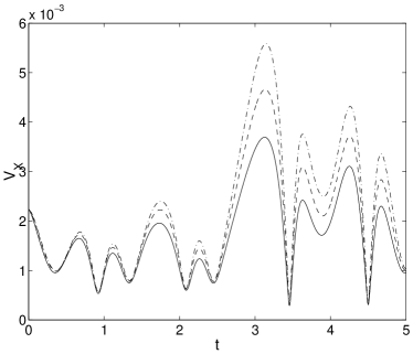
Figure 1: The standard deviations of the state estimates for each of the three observers for the Duffing oscillator, plotted over a duration of $t=5$. Solid line: observer with $\eta=0.5$; dashed line: observer with $\eta=0.3$; dash-dot line: observer with $\eta=0.2$.

V.1 The Duffing oscillator

The Duffing oscillator is a sinusoidally driven double-well potential, with Hamiltonian

$$H(t)=\frac{P^{2}}{2m}+BX^{4}-AX^{2}+\Lambda X\cos(\omega t)\,.$$ (57)

We choose $m=1$, $A=10$, $B=0.5$, $\Lambda=10$ and $\omega=6.07$. At times when the driving is zero, this puts the minima of the two potential wells at $\sim\pm 3.2$, with a central barrier height of $50$. We choose $\hbar=10^{-5}$ and $k=10^{5}$, which is sufficient to satisfy the inequalities derived in Section III for all but tiny values of $\eta$, and therefore puts the system in the classical regime. We now evolve the system with three observers, and set their measurement efficiencies to be $0.5,0.3,0.2$ respectively. We first calculate the position variance $V_{X}$ of the wave-function given by evolving Eq. (53)), and verify that this remains sufficiently small. Running the simulation for a duration of $t=5$, the maximum value of $\sqrt{V_{X}}$ is $2.7\times 10^{-3}$, and the rms value over the evolution is $1.4\times 10^{-3}$. The localization condition is therefore well satisfied, and an inspection of the evolution of the centroid shows that the noise is indeed negligible. Showing that the evolution is indeed the classical evolution is more nontrivial since the system is chaotic: any small difference in the noise on two trajectories will cause them to diverge rapidly, and one cannot therefore simply compare the trajectory to the equivalent noise-free classical trajectory. In Ref. BHJ1 , the classical dynamics was verified by comparing the stroboscopic map and the largest Lyapunov exponent obtained from the quantum evolution and their classical equivalents. Here we calculate the continuously estimated state, both quantum and classical, for the different observers, and show that these agree, and agree between observers.

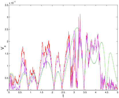
Figure 2: Plot of the error standard deviation (blue) and the difference between the estimated and true means for a single noise realization (red) for the simulation of the Duffing oscillator using the stochastic master equation with $\eta=0.5$. The green and purple curves plot the same quantities for the Gaussian estimator.

We now calculate the quantum state-estimate for each observer, obtained by integrating Eq. (55), and compare this with the classical (Gaussian) estimate for each observer, obtained by integrating Eqs. (48)-(52). In Figure 1 we plot the uncertainty in position (characterized by $\sqrt{V_{X}}=\sqrt{\mbox{Tr}[\rho X^{2}]-\mbox{Tr}[\rho X]^{2}}$) for the quantum state estimated by each observer over the duration of the run. All these remain small. The rms of $\sqrt{V_{x}}$ for each observer over the duration of the run is given in Table 1. The evolution of the uncertainty in position for the Gaussian state-estimate is essentially identical to the quantum estimate, and the rms of $\sqrt{V_{X}}$ for this estimate is also given in Table 1. Note that the position variances for each observer are, as expected, larger than the variance of the wave-function calculated using the stochastic Schrödinger equation. Since the solution to Eq. (53) can be viewed as an ‘unraveling’ of the stochastic master equation in Eq. (55), the difference between the variances of the ‘true’ state estimate from the former and the individual observers’ state estimate from the latter provides an estimate of the amount by which their means differ, averaged over noise realizations for all the observers. We will refer to this, for want of a better name, as the error variance, and its square root as the “error standard deviation”. The rms value of this error standard deviation is $1.2\times 10^{-3}$, $1.7\times 10^{-3}$ and $2.1\times 10^{-3}$ for observers with $\eta=0.5$, $0.3$ and $0.2$ respectively for both the stochastic master equation and Gaussian simulations. In Figure 2 we plot the evolution of the error standard deviation, and also the actual difference between the estimated mean and the mean of the wave-function, for both the master equation simulation and the Gaussian estimator. The small difference between these last two is most probably due solely to the fact that the mean of the computationally intensive master equation simulation has not completely converged at the value of the time step employed. (This difference is not seen for the computationally simpler delta-kicked rotor system discussed in the next subsection.)

Each observer may also track the position simply by averaging her measurement record over a suitable time period (i.e., by low pass filtering the measurement record). Naturally this period should be as long as possible so as to filter out the noise, but short enough so as not to filter out the deterministic motion. For this system we use a time period of $2.5\times 10^{-2}$ for the filtering. The average rms deviation of this estimate from the mean position of the wave-function is also given in Table 1 for each observer. From this we see that all observers can effectively track the motion of the particle (up to an error in position of about $10^{-2}$) using their measurement records directly.

Table 1: rms standard deviation of state-estimates for the Duffing oscillator and the rms deviation of the averaged measurement record.

Observer’s $\eta$	$\eta=0.5$	$\eta=0.3$	$\eta=0.2$
Quantum	$1.9\times 10^{-3}$	$2.3\times 10^{-3}$	$2.6\times 10^{-3}$
Gaussian	$1.9\times 10^{-3}$	$2.3\times 10^{-3}$	$2.6\times 10^{-3}$
Averaged Record	$8.2\times 10^{-3}$	$9.3\times 10^{-3}$	$1.1\times 10^{-2}$

V.2 The delta-kicked rotor

The delta-kicked rotor obeys the Hamiltonian

$$H(t)=\frac{P^{2}}{2m}+\kappa\cos(X)\sum_{n=0}^{\infty}\delta(t-n)\,.$$ (58)

It is, thus, a free particle, which experiences regular kicks from the potential of a nonlinear pendulum. For a wide range of parameters, the quantum behavior of this system (by which we mean the evolution of the closed system) is very different from the classical motion. In particular, after a few kicks the average energy of the closed classical system increases linearly with time. In the closed quantum system, however, the average energy reaches a maximum value and after that point remains fairly constant. This is termed dynamical localization. We now simulate the evolution of the observed wave-function for this system, with the same values of $\hbar$ and $k$ as we used for the Duffing oscillator, and with the same three observers. For the system parameters we will choose $\kappa=10$ and $m=1$, and integrate for a time period of 30 kicks. First we check the localization of the wave-function given by integrating the stochastic Schrödinger equation, and find that the average value of $\sqrt{V_{X}}$ is $2.1\times 10^{-3}$, and the maximum value obtained during the run is $3.2\times 10^{-3}$. We check that the mean energy is indeed behaving in a classical fashion by averaging this energy over many realizations, and comparing this to the classical value. In Figure 3 we plot the average energy of the observed quantum system, using $\hbar=0.1$ and $k=10$, along with both the classical result and the quantum result for $\hbar=0.1$.

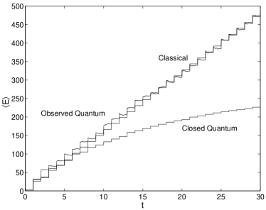
Figure 3: The average kinetic energy for the delta-kicked rotor as a function of time. The classical value is obtained by averaging over 10,000 trajectories. The observed quantum value was obtained by averaging over 1000 trajectories.

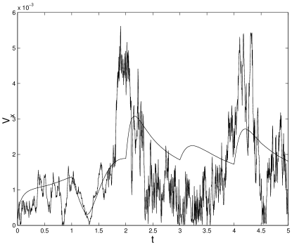
Figure 4: Plot of the error standard deviation (green) and the difference between estimated and true means for a single noise realization (red) for a simulation of the delta-kicked rotor using a stochastic master equation with $\eta=0.5$. The results for the Gaussian estimator are indistinguishable on this scale.

We next compare the position uncertainties in the state-estimates of the different observers, as above for the Duffing oscillator, and present these results in Table 2. The Gaussian estimator agrees with the stochastic master equation, and the uncertainties are small, so that the observers effectively all agree on the motion. The averaged measurement record also tracks the motion effectively. The rms value of the error standard deviation is $1.9\times 10^{-3}$, $2.9\times 10^{-3}$ and $3.7\times 10^{-3}$ for observers with $\eta=0.5$, $0.3$, and $0.2$ respectively. In figure 4 we plot the evolution of the error standard deviation for the observer with $\eta=0.5$ and also the actual difference between the estimated mean and the mean of the wave-function for a single realization of the stochastic master equation simulation. The equivalent plots for the Gaussian estimator are virtually indistinguishable.

To conclude, we see from the above simulations that (i) in the classical regime the full quantum state-estimation reduces to Gaussian state-estimation, and hence classical state-estimation may be used, (ii) even without the use of true (and therefore optimal) state-estimation, low pass filtering of the measurement record alone provides adequate tracking of the system, and (iii) since the errors in the respective estimates are small, all observers effectively agree upon the motion of the system.

Table 2: Average deviation of state-estimates for the delta-kicked rotor and the rms deviation of the averaged measurement record.

Observer’s $\eta$	$\eta=0.5$	$\eta=0.3$	$\eta=0.2$
Quantum	$2.9\times 10^{-3}$	$3.6\times 10^{-3}$	$4.3\times 10^{-3}$
Classical	$2.9\times 10^{-3}$	$3.6\times 10^{-3}$	$4.3\times 10^{-3}$
Averaged Record	$8.6\times 10^{-3}$	$1.0\times 10^{-2}$	$1.1\times 10^{-2}$

VI Conclusion

The emergence of classical dynamics remains a central issue in understanding the predictions of quantum mechanics, especially now that experiments are becoming available to probe this transition directly expts . In this paper, by deriving general inequalities which determine when classical mechanics will emerge, and by providing numerical examples, we have presented very substantial evidence that quantum measurement theory provides a completely satisfactory answer to the question of how classical mechanics, and hence classical chaos, emerges in a quantum world. In doing so we have shown in some detail how the mechanism for this transition can be understood as a result of localization and noise suppression in the classical regime.

While the emergence of classical dynamics for a single motional degree of freedom now appears to be well understood, the quantum to classical transition as yet holds many unanswered questions. What happens, for example, to the dynamics of a system as it passes “through” the transition? How do systems behave when they are neither fully quantum nor fully classical? For example, it is known that the delta kicked rotor demonstrates a complex behavior in the transition region BHJS . Further questions include how classical dynamics emerges for other degrees of freedom, such as spin, and what happens, for example, when spin and motional degrees of freedom are coupled? Must all the subsystems have a large action (we note that this has recently been investigated, see GADBHJ ), and must all the degrees of freedom be continuously measured, or will a subset suffice? For a spin system, must one measure all the components of spin, or will a single component suffice? Fortunately we are now at the point where one can not only pose these questions, but expect that solid answers will soon be forthcoming.

References

- (1) H.J. Korsch and M.V. Berry, Physica D 3, 627 (1981); T. Hogg and B.A. Huberman, Phys. Rev. Lett. 48, 711 (1982); R.L. Ingram, M.E. Goggin and P. W. Milonni, in Coherence and Quantum Optics VI, edited by J.H. Eberly (Plenum, New York, 1990).
- (2) A.O. Caldeira and A.J. Leggett, Physica A 121 587 (1983).
- (3) C.W. Gardiner and P. Zoller, Quantum Noise, 2nd edition (Springer, Berlin, 2000).
- (4) Early work includes A. Barchielli, L. Lanz, and G.M. Prosperi, Nuovo Cimento 72B, 79 (1982); N. Gisin, Phys. Rev. Lett. 52, 1657 (1984); L. Diosi, Phys. Lett. A 114, 451 (1986); for a review see, A. Barchielli, Int. J. Theor. Phys. 32, 2221 (1993).
- (5) V.P. Belavkin and P. Staszewski, Phys. Lett. A 40, 359 (1989).
- (6) C.M. Caves and G.J. Milburn, Phys. Rev. A 36, 5543 (1987).
- (7) H. Carmichael, An Open Systems Approach to Quantum Optics (Springer-Verlag, Berlin, 1993).
- (8) H.M. Wiseman and G.J. Milburn, Phys. Rev. A 47, 642 (1993).
- (9) K. Hepp, Helv. Phys. Acta 45, 237 (1972); W.H. Zurek, Phys. Rev. D 24, 1516 (1981); ibid 26, 1862 (1982); E. Joos and H.D. Zeh, Z. Phys. B 59, 223 (1985).
- (10) See, e.g., S. Habib, K. Shizume, and W.H. Zurek, Phys. Rev. Lett. 80, 4361 (1998).
- (11) T.P. Spiller and J.F. Ralph, Phys. Lett. A 194, 235 (1994).
- (12) M. Schlautmann and R. Graham, Phys. Rev. E 52, 340 (1995).
- (13) R. Schack, T.A. Brun, I.C. Percival, J. Phys. A 28, 5401 (1995); T.A. Brun, I.C. Percival, and R. Schack, J. Phys. A 29, 2077 (1996); I.C. Percival and W.T. Strunz, J. Phys. A, 31, 1815 (1998); J. Phys. A, 31, 1801 (1998);
- (14) T. Bhattacharya, S. Habib, and K. Jacobs, Phys. Rev. Lett. 85, 4852 (2000).
- (15) A.J. Scott and G.J. Milburn, Phys. Rev. A 63, 042101 (2001),
- (16) M. Brune, E. Hagley, J. Dreyer, X. Maitre, A. Maali, C. Wunderlich, J.M. Raimond, and S. Haroche, Phys. Rev. Lett. 77, 4887 (1996); C.J. Hood, M.S. Chapman, T.W. Lynn, and H.J. Kimble, ibid. 80, 4157 (1998); H. Ammann, R. Gray, I. Shvarchuck, and N. Christensen, ibid. 80, 4111 (1998); B.G. Klappauf, W.H. Oskay, D.A. Steck, and M.G. Raizen, ibid. 81, 1203 (1998).
- (17) C.W. Gardiner, Stochastic Methods (Springer-Verlag, Berlin, 1990).
- (18) G.J. Milburn, K. Jacobs, and D.F. Walls, Phys. Rev. A 50 5256 (1994).
- (19) A.C. Doherty and K. Jacobs, Phys. Rev. A 60, 2700 (1999).
- (20) The ‘if’ part of the statement is clear from early work in Ref. cqm1 . The ‘only if’ is clear by noting that if is an one-dimensional projector (so that ) that is not into an eigenspace of , implies averaged over the noise is positive definite.
- (21) This follows most simply by treating each observer as having access to a separate output channel, or environment, but it is clear from HMW that one could obtain the same result by dividing up the available light using a sequence of beam splitters. For an explicit treatment of multiple observers see reference Barch93 . A recent and less mathematical treatment is also given in reference DDZ .
- (22) H.M Wiseman, PhD Thesis (University of Queensland)
- (23) A. Barchielli, Int. J. Theor. Phys. 32, 2221(1993).
- (24) J. Dziarmaga, D.A.R Dalvit, and W.H. Zurek quant-ph/0107033.
- (25) S. Habib, in preparation.
- (26) Positivity at this second cumulant level does not require the noise term: the covariance matrix stays positive even without the addition of this piece.
- (27) Since complex conjugation along with leaves the algebra unchanged, the momentum flip along with (i.e., and ) and is an invariance of Eq. 3. Thus our results also apply to the negative mass case mutatis mutandis.
- (28) P.S. Maybeck, Stochastic Models, Estimation and Control, (Academic Press, New York, 1982).
- (29) A.C. Doherty, S. Habib, K. Jacobs, H. Mabuchi, and S.M. Tan, Phys. Rev. A 62, 012105 (2000).
- (30) T. Bhattacharya, S. Habib, K. Jacobs and K. Shizume, Phys. Rev. A 65, 032115 (2002)
- (31) S. Ghose, P.M. Alsing, I.H. Deutsch, T. Bhattacharya, S. Habib, K. Jacobs, quant-ph/0208064.