Efficient implementations of the Quantum Fourier Transform: an experimental perspective

Abstract

The Quantum Fourier transform (QFT) is a key ingredient in most quantum algorithms. We have compared various spin-based quantum computing schemes to implement the QFT from the point of view of their actual time-costs and the accuracy of the implementation. We focus here on an interesting decomposition of the QFT as a product of the non-selective Hadamard transformation followed by multiqubit gates corresponding to square- and higher-roots of controlled-NOT gates. This decomposition requires only $O(n)$ operations and is thus linear in the number of qubits $n$. The schemes were implemented on a two-qubit NMR quantum information processor and the resultant density matrices reconstructed using standard quantum state tomography techniques. Their experimental fidelities have been measured and compared.

I Introduction

The Fourier transform finds widespread application in physics and information processing, and it comes as no surprise that its quantum version lies at the core of most known quantum computational algorithms. The Quantum Fourier Transform (QFT) is analogous to the classical Fast Fourier Transform (FFT), and by exploiting the advantages of quantum parallelism, can be computed exponentially faster. However, this advantage cannot be used to speed up data processing tasks, since the individual Fourier transformed output amplitudes cannot be accessed by a measurement. What the QFT can achieve is an estimation of arbitrary quantum phases and an extraction of the periodicity of a function. Indeed, fast quantum algorithms for factoring shor ; ekert-proc ; jozsa-proc , finding discrete logarithms simon and the more general algorithm for finding the stabilizer of an Abelian group kitaev , rely crucially on this property of the QFT.

Schemes to implement the QFT have been proposed using cavity QED scully-qed and have been experimentally implemented using NMR cory1 ; chinese1 ; cory2 ; chinese2 . Despite several limitations (see for example the points made in jones-review ; cory-review and similar reviews), NMR remains to date the only existing quantum-computing technology. However, with ideas for quantum algorithms that work with expectation-value quantum computers glaser ; collins and proposals for scalable solidstate NMR quantum computing implementations kane ; suter ; yamamoto , it is likely that spin-based implementations will soon emerge as a viable technology for quantum computing.

The key role played by the QFT in quantum algorithms makes it an attractive candidate for detailed investigations of its experimental implementations. Issues of the actual time-cost of quantum algorithms as compared to their ideal computational cost have seldom been quantitatively addressed saito ; barenco . However, these issues are relevant and need to be tackled for technology to keep pace with theoretical developments. This paper seeks to compare different decompositions of the QFT, with a view to finding the most efficient experimental spin-based quantum computing implementation.

II The QFT and its decompositions

The basis states that we consider are product states

$$|a\rangle=|a_{n-1}a_{n-2}...a_{0}\rangle=|a_{n-1}\rangle_{n-1}\otimes...|a_{1}\rangle_{1}\otimes|a_{0}\rangle_{0},$$

which can be represented by binary integers

$$a=\sum_{j=0}^{n-1}a_{j}2^{j},a_{j}\in\{0,1\}.$$

q = $2^{n}$ is the dimension of the Hilbert space and $n$ the number of qubits.

In this basis, the QFT can be represented as a unitary operator $\mathcal{F}$, which transforms the basis states $|a\rangle$ into

$$\mathcal{F}|a\rangle=\frac{1}{\sqrt{q}}\sum_{c=0}^{q-1}e^{2\pi iac/q}|c\rangle.$$ (1)

The states $|c\rangle$ have the same form as $|a\rangle$.

When applied to an arbitrary state $|\psi\rangle=\sum_{a}A_{a}|a\rangle$, the QFT yields

$$\mathcal{F}|\psi\rangle\equiv\mathcal{F}\sum_{a=0}^{q-1}A_{a}|a\rangle\longrightarrow\sum_{c=0}^{q-1}C_{c}|c\rangle$$ (2)

where the coefficients $C_{c}$ are the discrete Fourier transform of the input coefficients $A_{a}$.

The basis transformation of Eqn. 1 can be written in terms of individual qubits as

$$\mathcal{F}|a\rangle=\prod_{j=0}^{n-1}\otimes|p(\phi_{j})\rangle_{j}$$ (3)

where each qubit is in a state $|p(\phi_{j})\rangle=(|0\rangle+e^{i2\pi\phi_{j}}|1\rangle)/\sqrt{2}$. The phases are determined by

$$\phi_{j}=\sum_{k=0}^{n-1-j}a_{k}2^{j+k-n}$$

Equation 3 serves as the basis for implementing the QFT by one- and two-qubit operations. One implementation barenco ; coppersmith ; griffiths uses single-qubit Hadamard rotations gates $H_{j}$ and two-qubit controlled-phase gate $B_{j,k}$ that act on the qubits $j$ and $k$ and are given by

$$B_{j,k}=\left(\begin{array}[]{cccc}1&0&0&0\\ 0&1&0&0\\ 0&0&1&0\\ 0&0&0&e^{i\theta_{jk}}\end{array}\right)$$

where $\theta_{jk}=\pi 2^{j-k}$ is a conditional phase shift applied only if both qubits are in the state $|1\rangle$. In terms of these gates, the quantum circuit for $n$ qubits is

$$\mathcal{QFT}_{n} = (H_{1}B_{1,2}...B_{1,n})(H_{2}B_{2,3}...B_{2,n})...$$ (4)

$$...(H_{n-1}B_{n-1,n})(H_{n})$$

with the sequence of operations being performed from right to left. With this implementation, the bit values of the result appear in reversed order. If a sequence reversal is required, this can be achieved by a sequence of SWAP operations on pairs of qubits.

We shall denote this decomposition of the QFT, as “serial”. For $n$ qubits, it requires a total of $n$ $H_{j}$ gates, $n(n-1)/2$ $B_{j,k}$ gates and $n/2$ SWAP operations, leading to a computational complexity of $O(n^{2})$.

Individual Hadamard operations are qubit-selective and hence costlier than a total Hadamard operator that is applied on all qubits simultaneously. It would be thus desirable to have a decomposition of the QFT that involves a non-selective Hadamard transformation cory2 .

Figure 1: (a) Quantum circuit for the serial implementation of the QFT using qubit-selective Hadamard rotations and two-qubit controlled-phase gates. (b) Circuit for the parallel implementation of the QFT using a non-selective Hadamard rotation on all qubits, and multiqubit gates. The readout of the QFT is performed in reverse order on the qubits, achieved by SWAP operations (not shown in the circuits).

A more useful (for NMR) decomposition of the QFT can be obtained by noting that the Hadamard operator is self-inverse and that a Hadamard rotation of the controlled-phase gate can be decomposed as a root of a controlled-NOT gate ,

$$H_{k}B_{jk}H_{k}^{-1}=e^{i\pi/2^{k-j+1}}(U_{CNOT})^{1/2^{k-j}}_{j,k}$$

where $j$ is the control and $k$ the target qubit. The global phase factor does not influence measurement results and is henceforth ignored. Further, using

$$[H_{i},B_{j,k}]=0,i\neq j,k,$$

the sequence of operations in Eqn. (4) can be modified to

$$\mathcal{QFT}_{n}=[H_{T}][U_{1}U_{2}...U_{n-2}U_{n-1}]$$ (5)

where

$$H_{T}=H_{1}H_{2}H_{3}...H_{n-1}H_{n}$$

is the total non-selective Hadamard operator on all qubits, i.e. a single $\pi/2$ radio frequency pulse.

The $U$ gates in Eqn. (5) are

$$U_{1} = H_{2}B_{1,2}H_{2}^{-1}$$

$$= (U_{CNOT})^{1/2}_{1,2}$$

$$U_{n-2} = H_{n-1}(B_{1,n-1}B_{2,n-1}...B_{n-2,n-1})H_{n-1}^{-1}$$

$$= (U_{CNOT})^{1/2^{n-2}}_{1,n-1}(U_{CNOT})^{1/2^{n-3}}_{2,n-1}..(U_{CNOT})^{1/2}_{n-2,n-1}$$

$$U_{n-1} = H_{n}(B_{1,n}B_{2,n}...B_{n-1,n})H_{n}^{-1}$$

$$= (U_{CNOT})^{1/2^{n-1}}_{1,n}(U_{CNOT})^{1/2^{n-2}}_{2,n}..(U_{CNOT})^{1/2}_{n-1,n}$$

They correspond to single spin rotations conditioned on the status of all the other spins involved in the operation. Since they are single spin rotations, they can be implemented as single radio frequency pulses. The conditioning on the state of the other spins is achieved by making them selective on specific transitions. As an example, for a system of three qubits, the operation $U_{n-1}$ in this case is given by a fourth-root of a controlled-NOT gate on qubits one and three, followed by a square-root of a controlled-NOT gate on qubits two and three, with the third qubit being the target qubit in both cases. These gates thus involve three transitions of the third qubit: $100\rightarrow 101,110\rightarrow 111$, and $010\rightarrow 011$. Since these are unconnected transitions, rotations in the subspace of these transitions can be achieved simultaneously. Many pulsed irradiation schemes for such precise selective excitation exist in NMR, mostly involving shaping the excitation profile of the rf waveform cory-newsel . The entire QFT operation in this decomposition therefore reduces to a sequence of $n$ radio frequency pulses. It scales linearly with the number of qubits, and we will denote it as the “parallel” implementation.

III Time-Cost of the QFT

The main issue in the experimental implementation of quantum algorithms is not the number of logical operations per se, but the actual time-cost of each logical operation/quantum gate. The $U$ transformations in Eqn. (5) are no longer two-qubit phase-shift gates but correspond to square- and higher-roots of controlled-NOT operations on specific qubits. They can be implemented experimentally using multiqubit gates that perform manipulations on qubits simultaneously. Since the NMR Hamiltonian has terms connecting multiple pairs of qubits, such multiqubit gates can be directly implemented. The quantum circuits for both serial and parallel implementations of the QFT are shown in Figure 1.

The most expensive operation in the serial implementation of the QFT is the controlled-phase shift gate $B_{jk}$. The ideal time-cost is computed assuming all gates take the same amount of time. However experimentally, the controlled-phase shift gate requires a time $\tau_{jk}$ proportional to the desired phase rotation angle $\theta_{jk}$ (related to the “distance” $(k-j)$ of the qubits), and inversely proportional to the interaction $J_{jk}$ between the qubits. The magnitude of the interaction $J_{jk}$ and hence the time cost depends on the specific experimental quantum computing technology under consideration. For liquid-state NMR, $J_{jk}$ is the electron-mediated scalar coupling between the qubits. For our calculations, we assume the $J_{jk}$’s to be of the same order of magnitude for all qubits, represented by a universal constant coupling $J$. The actual time cost of the serial decomposition of the QFT, involving only one-qubit Hadamards and the two-qubit phase-controlled gate is

$$T_{ser}=n\delta+\sum_{j=0}^{n-1}\sum_{k=j+1}^{n}\tau_{jk} = n\delta+\kappa\sum_{j=0}^{n-1}\sum_{k=j+1}^{n}2^{j-k}$$ (7)

$$= n\delta+\kappa(n-1+2^{-n})$$

$$\approx O(n)$$

where $\delta$ is the time-cost of each single-qubit Hadamard rotation and $\kappa=\pi/J$. Using multiqubit gates in the parallel implementation of the QFT reduces the actual time-cost of the algorithm. Quite apart from the saving obtained by using a non-selective Hadamard transformation in the beginning on all the qubits, each $U$ gate can be thought of as having components from one or more $B_{jk}$ gates. The actual time-cost of the parallel QFT is

$$T_{par}=\kappa\sum_{j=0}^{n-1}\sum_{k=j+1}^{n}\tau_{jk}$$ (8)

Since for multiqubit gates, the system evolves under more than one coupling period simultaneously, only the largest of these need be counted for contribution to the time-cost and the inner sum in Eqn. (8) vanishes to give

$$T_{par}=\kappa\sum_{j=0}^{n-1}2^{-1}=\kappa n/2\approx O(n)$$ (9)

The analysis does not include the degradation of each gate due to decoherence nor does it take into account the SWAP operations, since the latter can in most cases be avoided by a relabeling of qubits. Implementing the Approximate QFT barenco would require fewer controlled-phase gates but would correspondingly reduce the accuracy.

IV NMR Implementations of the QFT

Experiments were performed on a de-gassed, flame-sealed sample of ¹³C-labeled chloroform, with ¹³C and ¹H as the two qubits and a coupling constant of $J_{12}\approx 215$Hz. Qubit-selective $90$ degree pulses are of the order of $10\mu s$. The unitary transformations required for the parallel decomposition of the QFT can be implemented either by transition-selective pulses or by J-coupling intervals sandwiched between qubit-selective pulses. A low-power rectangular pulse of length $6.5ms$ was used to selectively excite individual transitions for the selective implementation of the QFT. For heteronuclear systems, RF pulses are applied on two different channels, leading to a reduction in the duration of selective pulses.

Each version of the QFT was implemented on a temporally averaged pseudopure state temp-avg , obtained from the thermal equilibrium ensemble as the sum of three experiments

$${\bf E}\,\,\,\,\,\,\,\,\mbox{(do-nothing operation)}$$

$$\{90_{x}\}^{C}\frac{1}{2J_{12}}\{90_{y}\}^{C}\{90_{x}\}^{H}\frac{1}{2J_{12}}\{90_{y}\}^{H}$$

$$\{90_{x}\}^{H}\frac{1}{2J_{12}}\{90_{x}\}^{C}\{90_{y}\}^{H}\frac{1}{2J_{12}}\{90_{y}\}^{C}$$

The details of the pulse sequences used to implement the serial, parallel and the selective-pulse (parallel) decompositions of the QFT, are given in Table 1. The final SWAP operation was not executed; instead the readout in the reverse order was achieved by “relabeling” the qubits at the end of each experiment.

The results of all three implementations of the QFT are shown in Figure 2, using three-dimensional bar graphs to represent components of the final density matrix. Since only single-quantum terms are observable in NMR, it is necessary to perform a series of experiments that rotate unobservable terms into observable ones, in order to sample the entire density matrix. The density matrix after each implementation of the QFT was reconstructed by standard quantum state tomography procedures, using a set of nine experiments and qubit-selective readouts tomo ; tomo-chinese .

The precision of the QFT implementation can be estimated by measuring its “fidelity”, defined for mixed density matrices (such as the ones encountered in NMR) cory1

$$F=\frac{Tr(\rho_{th}\rho_{exp})}{\sqrt{Tr(\rho^{2}_{th})}\sqrt{Tr(\rho^{2}_{exp})}}\sqrt{\frac{Tr(\rho^{2}_{exp})}{Tr(\rho^{2}_{init})}}$$

The first term in the expression measures the correlation between the experimental deviation density matrix $\rho_{exp}$ and the theoretical deviation density matrix $\rho_{th}$ (obtained by “applying” the unitary operator corresponding to the ideal QFT transformation, to the initial density matrix $\rho_{init}$). The second term is the weighting factor to take into account the overall signal loss due to decoherence during the experiment.

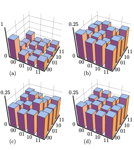
Figure 2: The experimental deviation density matrices (a) for the pseudopure state $|00\rangle$ and for the states obtained after applying the QFT to the pseudopure state using the pulse sequence for (b) the selective implementation (c) the parallel implementation and (d) the serial implementation of the QFT. The rows are labelled in the standard computational basis.

The fidelities measured for the serial, parallel and selective-pulse versions of the QFT are $79\%$, $80\%$ and $85\%$ respectively. The reduction in fidelity is mainly due to imperfections in pulse calibration as well as system decoherence. It is not surprising that the serial and parallel versions are equally accurate for the case of two qubits. The savings in time and the increase in accuracy of the parallel QFT will be realised only for a larger number of qubits. The better performance of the selective scheme is due to the fact that such a direct implementation of the square-root of the controlled-NOT gate does not require refocusing schemes freeman ; kd . However, in systems with a larger number of qubits such selective pulse schemes might not be feasible, the major stumbling blocks in such cases being decoherence during the pulses and the overlap of transitions in crowded spectra.

V Other spin-based architectures

Recently, several approaches have been suggested for the design of solid-state spin-based quantum computers. Kane’s proposal kane using single donor spins in Si, addresses the problem of scalability but has the disadvantages inherent in single-spin measurements. Ladd et. al.’s solid-state NMR quantum computing device on the other hand, is made entirely of silicon, with the qubits being spin-1/2 nuclei located in isolated atomic chains yamamoto . Suter et. al. suter proposed an alternative architecture with each logical qubit being represented by two physical qubits - an active electron spin to manipulate quantum information and a passive nuclear spin to store information. A logical qubit is addressed using magnetic field gradients and SWAP gates, realised as a cascade of three transition-selective pulses, are used to convert between active and passive states. A basic two-qubit gate relies on the dipolar interaction between electron spins and requires four additional SWAP gates, two to switch between active and passive states and two back-SWAPS to switch off the interaction between the neighbouring qubits. The hyperfine interaction is of the order of a few MHz and the electron dipolar interaction strength is around 10-50 MHz. An estimate of the actual time-cost of the QFT for such a solid-state spin quantum computer yields

$$T_{ser} = n\delta+\sum_{j=0}^{n-1}\sum_{k=j+1}^{n}(\tau_{jk}+2*\tau_{\tiny SWAP})$$ (10)

$$= n\delta+2n\Delta+\kappa\sum_{j=0}^{n-1}\sum_{k=j+1}^{n}2^{j-k}$$

$$= n\delta+2n\Delta+\kappa(n-1+2^{-n})\approx O(n)$$

where $\delta$ is the time-cost of each single-qubit Hadamard rotation, $\kappa=\pi/d$, $d$ is the strength of the dipolar interaction and $\Delta$ is the time unit of one SWAP gate. Since the gate times for this implementation are very fast, a greater number of logical operations compared to liquid-state NMR computers, can be performed within the system decoherence limit. These solid-state proposals are also scalable to a very large number of qubits.

In conclusion, we have estimated the realistic time-costs of different decompositions of the QFT for liquid and solid-state NMR quantum computers and have measured the accuracy of the implementations experimentally using liquid-state NMR. While all quantum computation can be implemented using the two-qubit universal controlled-NOT gate and one-qubit rotations, the number of these basic operations increases exponentially with the number of qubits. It has been suggested that for some specific QC purposes, using more complicated multiqubit gates might be computationally more efficient multiqubit1 ; multiqubit2 . The parallel implementation of the QFT suggested by Cory et. al., using multiqubit gates, performs better than the serial implementation. The actual experimental time-costs can be improved upon using innovative techniques like multiqubit gates, creative refocusing schemes refocus and time-optimal gates designed using control theory glaser-control ; chinese-control .

Table 1: NMR pulse schemes for different implementations the QFT on $n=2$ and 3 qubits. Superscript $r\rightarrow s$ indicates a selective RF pulse on the transition $r\rightarrow s$. Superscripts $r$ and $r,s$ indicate spin-selective pulses on the spins $r$ and $r,s$ respectively. Subscript $z$ indicates a composite-z pulse which can be expanded as a sandwich of rf pulses $\{\theta_{z}\}\equiv\{90_{x}\}\{\theta_{y}\}\{90_{x}\}$.

Implementation	$n=2$	$n=3$
Serial QFT	$\{90_{y}\}^{1}\{180_{x}\}^{1}\frac{1}{4J_{12}}\{90_{y}\}^{1,2}\{45_{x}\}^{1,2}$	$\{45_{y}\}^{3}\{180_{x}\}^{3}\{45_{-y}\}^{3}\{180_{x}\}^{3}\frac{1}{4J_{23}}$
	$\{90_{-y}\}^{1,2}\{90_{y}\}^{2}\{180_{x}\}^{2}$	$\{180_{-x}\}^{3}\{90_{y}\}^{2,3}\{45_{x}\}^{2,3}\{90_{-y}\}^{2,3}\{45_{y}\}^{2}$
		$\{180_{x}\}^{2}\{45_{-y}\}^{2}\{180_{x}\}^{1}\frac{1}{8J_{13}}\{180_{-x}\}^{1}$
		$\{90_{y}\}^{1,3}\{22.5_{x}\}^{1,3}\{90_{-y}\}^{1,3}\{180_{x}\}^{2}\frac{1}{4J_{12}}$
		$\{180_{x}\}^{2}\{90_{y}\}^{1,2}\{45_{x}\}^{1,2}\{90_{-y}\}^{1,2}\{45_{y}\}^{1}$
		$\{180_{x}\}^{1}\{45_{-y}\}^{1}$
Parallel QFT	$\{90_{y}\}^{1,2}\{180_{x}\}^{1,2}\{90_{y}\}^{2}\{180_{x}\}^{1,2}\frac{1}{4J_{12}}$	$\{45_{y}\}^{1,2,3}\{180_{x}\}^{1,2,3}\{45_{-y}\}^{1,2,3}\{90_{-y}\}^{2}\frac{1}{4J_{23}}$
		$\{90_{y}\}^{2}\{45_{x}\}^{2}\{180_{x}\}^{1}\{90_{y}\}^{1,2}\{45_{x}\}^{1,2}$
		$\{90_{-y}\}^{1}\{180_{x}\}^{2}\{90_{-y}\}^{1}\{\frac{1}{4J_{12}},\frac{1}{8J_{13}}\}\{90_{y}\}^{1}$
		$\{67.5_{x}\}^{1}\{135_{-z}\}^{3}\{90_{-z}\}^{2}$
Selective-pulse	$\{90_{y}\}^{1,2}\{180_{x}\}^{1,2}\{90_{x}\}^{3\rightarrow 4}\{45_{z}\}^{1}$	$\{90_{y}\}^{1,2,3}\{180_{x}\}^{1,2,3}\{90_{x}\}^{6\rightarrow 8}\{90_{x}\}^{5\rightarrow 7}$
(parallel QFT)		$\{180_{x}\}^{7\rightarrow 8}\{90_{x}\}^{5\rightarrow 6}\{90_{x}\}^{3\rightarrow 4}\{67.5_{z}\}^{1}\{45_{z}\}^{2}$

- (1) P. W. Shor, SIAM J. Comput., 26, 1484 (1997).
- (2) R. Cleve, A. Ekert, C. Macchiavello, and M. Mosca, Proc. R. Soc. A, 454, 339 (1998).
- (3) R. Jozsa, Proc. R. Soc. A, 454, 323 (1998).
- (4) D. R. Simon, SIAM J. Comput., 26, 1474 (1997).
- (5) A. Y. Kitaev, quant-ph/9511026 (1995).
- (6) M. O. Scully and M. S. Zubairy, Phys. Rev. A, 65, 052324 (2002).
- (7) Y. S. Weinstein, S. Lloyd, and D. G. Cory, Phys. Rev. Lett., 86, 1889 (2001).
- (8) L. Fu, J. Luo, L. Xiao, and X. Zheng, quantph/9905083 (1999).
- (9) M. D. Price, T. F. Havel, and D. G. Cory, New J. Phys., 2, 101 (2000).
- (10) X. Peng, X. Zhu, X. Fang, M. Feng, X. Yang, M. Liu, and K. Gao, quant-ph/0202010 (2002).
- (11) J. A. Jones, Fortschr. Phys., 48, 909 (2000).
- (12) D. G. Cory, R. Laflamme, E. Knill et. al., Fortschr. Phy., 48, 875 (2000).
- (13) J. M. Myers, A. F. Fahmy, S. J. Glaser, and R. Marx, Phys. Rev. A, 63, 032302 (2001).
- (14) D. Collins, Phys. Rev. A, 65, 052321 (2002).
- (15) B. E. Kane, Fortschr. Phys., 48, 1023 (2000).
- (16) T. D. Ladd, J. R. Goldman, F. Yamaguchi, and Y. Yamamoto, Phys. Rev. Lett., 89, 017901 (2002).
- (17) D. Suter and K. Lim, Phys. Rev. A, 65, 052309 (2002).
- (18) A. Saito, K. Kioi, Y. Akagi, N. Hashizume, and K. Ohta, quant-ph/0001113 (2000).
- (19) A. Barenco, A. Ekert, K-A. Suominen, and P. Torma, Phys. Rev. A, 54, 139 (1996).
- (20) D. Coppersmith, IBM Res. Rep., RC 19642 (1994).
- (21) R. B. Griffiths and C-S. Niu, Phy. Rev. Lett., 76, 3228 (1996).
- (22) E. M. Fortunato, M. A. Pravia, N. Boulant, G. Teklemariam, T. F. Havel, and D. G. Cory, J. Chem. Phys., 116, 7599 (2002).
- (23) E. Knill, I. Chuang, and R. Laflamme, Phys. Rev. A, 57, 3348 (1998).
- (24) I. L. Chuang, N. Gershenfeld, M. G. Kubinec, and D. W. Leung, Proc. R. Soc. A, 454, 447 (1998).
- (25) G. L. Long, H. Y. Yan, and Y. Sun, J. Opt. B, 3, 376 (2001).
- (26) N. Linden, H. Barjat, and R. Freeman, Chem. Phys. Lett., 296, 61 (1998).
- (27) K. Dorai, Arvind, and A. Kumar, Phys. Rev. A, 61, 042306 (2000).
- (28) M. D. Price, S. S Somaroo, A. E. Dunlop et. al., Phys. Rev. A, 60, 2777 (1999).
- (29) J. F. Du, M. J. Shi, J. H. Wu et. al., Phys. Rev. A, 63, 042302 (2001).
- (30) J. A. Jones, and E. Knill, J. Magn. Res., 141, 322 (1999).
- (31) N. Khaneja, S. J. Glaser, and R. Brockett, Phys. Rev. A, 65, 032301 (2002).
- (32) R. Wu, C. Li and Y. Wang, Phys. Lett. A, 295, 20 (2002).