Complex Optical Potentials and Pseudo-Hermitian Hamiltonians

Abstract

Recently some authors have broadened the scope of canonical quantum mechanics by replacing the conventional Hermiticity condition on the Hamiltonian by a weaker requirement through the introduction of the notion of pseudo-Hermiticity. In the present study we investigate eigenvalues, transmission and reflection from complex optical potentials enjoying the property of pseudo-Hermiticity.

, ,

Bender, his collaborators and others [1-23] in a series of papers, investigated some non-Hermitian Hamiltonians which violate parity $(P)$ and time reversal $(T)$ symmetry but are $PT$ invariant. These systems comprised of a particle moving in a complex potential, the real part of which is parity-even while the imaginary part is odd. Through various examples it was found that the energy eigenvalues were real and bounded from below. Though in some cases, for a range of parameters (contained in the potential), complex eigenvalues do occur, but these are associated with a spontaneous breaking of $PT$ symmetry. Subsequently Mostafazadeh [24] has provided a basic mathematical setting for such systems by introducing the notion of pseudo-Hermiticity of the Hamiltonian $H$ via the condition $H^{\dagger}={\eta}H{\eta}^{-1}$ where ${\eta}$ is a Hermitian, linear and invertible operator. It is suitable to define an indefinite inner product of two state vectors: ${\ll}{\psi}_{1}{|}{\psi}_{i}{2}{\gg}_{\eta}$ = ${\langle}{\psi}_{1}{|}{\eta}{|}{\psi}_{2}{\rangle}$ which is time translationally invariant with $\eta$ playing the role of a metric operator in Hilbert space. One can then go on to show that the eigenvalues of $H$ are either real or occur as complex conjugate pairs and the eigenvectors constitute a complete biorthonormal system. For the examples considered by Bender and others $\eta$ is the parity operator $(\eta=P)$.

In the present study we attempt to put such Hamiltonians in a more ‘physical’ setting and moreover extend the discussion to continuum states as well. We encounter some rather amusing features. We recall [25] the optical (or cloudy crystal ball) model of the atomic nucleus, where the interaction of a neutron (or some other projectile) with the nucleus is described through a complex potential $V+iW$, where $V$ and $W$ are its real and imaginary parts respectively. From the continuity equation obeyed by the probability and probability current densities (following from Schrödinger equation) it is easily seen that non-vanishing $W$ implies a sink (or source) for the probability, depending on the sign of $W$, which is taken to correspond to absorption (or emission) of particles with respect to the incident beam, and this furnishes a rather useful phenomenological description of elastic scattering in the presence of open inelastic channels. In one of the versions of this picture, known as the surface absorption model, the imaginary part $(W)$ of the potential is taken to be proportional to the spatial derivative (gradient) of the real part $(V)$. We shall see that a one-dimensional ‘cartoon’ of the surface absorption version of the optical model leads naturally to a $PT$-invariant (or more appropriately a pseudo-Hermitian) Hamiltonian. We illustrate some novel features of pseudo-Hermitian Hamiltonians through two examples so chosen such that the results are expressible in terms of elementary functions.

Consider a particle of mass $m$ moving in one dimension under the influence of a potential the real part $(V)$ of which is an attractive square well of depth $V_{0}$ and range $a$ and whose imaginary part $(W)$ is proportional to the derivative of the real part. Accordingly the motion is governed by the Hamiltonian

$$H=\frac{p^{2}}{2m}+V+iW=\frac{p^{2}}{2m}-V_{0}\theta(\frac{a}{2}-{|}x{|})+i{\lambda}[\delta(x-\frac{a}{2})-\delta(x+\frac{a}{2})].$$ (1)

Note that the Hamiltonian is not parity invariant as $V+iW{\longrightarrow}V-iW$ ($W$ being an odd function of $x$ ), nor is it time reversal invariant as the operation of complex conjugation takes $V+iW{\longrightarrow}V-iW$. However the system enjoys symmetry under the combined $PT$ transformation. More relevantly the Hamiltonian is pseudo-Hermitian viz. $H^{\dagger}=PHP^{-1}$ with the parity operator $P$ being allowed to play the role of the ‘metric’ operator $(\eta)$ in the Hilbert space.

Analysing the bound state situation to begin with, it is convenient to put the energy eigenvalue $E=-B$ with $B>0$ and to define $\frac{2mB}{{\hbar}^{2}}={\beta}^{2}$, so that ${\psi}_{I}(x)=A{e^{{\beta}x}}$ for $x<-{\frac{a}{2}}$ (as $\psi$ must vanish as $x{\longrightarrow}-{\infty}$) and $\psi_{III}(x)=D{e^{-{\beta}x}}$ in the region $x>+\frac{a}{2}$ (as $\psi$ must vanish as $x{\longrightarrow}+{\infty}$). In the range ${|}x{|}<\frac{a}{2}$ we have the solution $\psi_{II}(x)=C_{1}e^{iqx}+C_{2}e^{-iqx}$ where $q^{2}=\frac{2m(V_{0}-B)}{\hbar^{2}}$. Implementing the continuity and jump conditions $\psi_{I}(\frac{-a}{2})=\psi_{II}(\frac{-a}{2})$, $\psi_{II}(\frac{+a}{2})=\psi_{III}(\frac{+a}{2})$, $\psi_{II}^{\prime}({\frac{-a}{2}})-\psi_{I}^{\prime}({\frac{-a}{2}})=-i\tilde{\lambda}{\psi_{I}}({\frac{-a}{2}})$, $\psi_{III}^{\prime}(\frac{+a}{2})-{\psi_{II}}^{\prime}({\frac{+a}{2}})=i\tilde{\lambda}{\psi_{III}}({\frac{+a}{2}})$ where $\tilde{\lambda}~{}~{}~{}{\equiv}~{}~{}~{}{\frac{2m{\lambda}}{\hbar^{2}}}$, we arrive at the eigenvalue condition

$$(q^{2}-{\beta^{2}}-{\tilde{\lambda}^{2}})~{}~{}Sin(qa)=2{\beta}q~{}~{}Cos(qa).$$ (2)

Before going on to a discussion of the solution to this equation, it is revealing to ask the question: Is there a minimum depth $V_{0}$ below which a bound state (with the usual meaning of the concept as elaborated below) does not exist ? For the square well potential (with $\lambda=0$) we know that there is at least one bound state howsoever weak the attraction ( given by $V_{0}$ ) may be. Also for $\sqrt{\frac{2mV_{0}a^{2}}{\hbar^{2}}}<\frac{\pi}{2}$ there is only one bound state. Let us choose the real part of the potential to lie in this region ( say $\frac{2mV_{0}a^{2}}{\hbar^{2}}=1$ ) and look for the effect of the imaginary part ($\lambda$) on the binding energy by numerically solving eq.(2). The result is shown graphically in $Fig.1(a)$. Observe that the binding energy goes to zero at $\tilde{\lambda}\equiv\frac{2m\lambda}{\hbar^{2}}=1$. This is readily seen by looking at the zero binding condition, namely, $\beta=0$ in the eigenvalue equation [eq. (2)] which yields the relation

$$(V_{0}-{\frac{2m{\lambda^{2}}}{\hbar^{2}}})Sin({\sqrt{\frac{2mV_{0}}{\hbar^{2}}}}a)=0.$$ (3)

The relevant result for this minimum depth is thus

$$V_{0}=\frac{2m{\lambda}^{2}}{\hbar^{2}}.$$ (4)

In this limiting situation the wavefunction corresponding to zero binding $(B=0)$ is

${\psi_{I}}=A$     for $x<-{\frac{a}{2}}$,

${\psi_{II}}=Ae^{-i{\frac{m{\lambda}a}{\hbar^{2}}}-i\frac{2m{\lambda}x}{\hbar^{2}}}$     for -${\frac{a}{2}}<x<+{\frac{a}{2}}$

${\psi_{III}}=Ae^{-i{\frac{2m{\lambda}a}{\hbar^{2}}}}$     for $x>+{\frac{a}{2}}$.

To examine analytically what happens when the strength of imaginary part crosses the critical value, let us choose for simplicity $\sqrt{\frac{2mV_{0}a^{2}}{\hbar^{2}}}=\frac{\pi}{2}$ and look in the neighbourhood of the point ${\tilde{\lambda}}^{2}=\frac{2mV_{0}}{\hbar^{2}}={\omega}^{2}$ viz ${\tilde{\lambda}}^{2}a^{2}={\omega}^{2}a^{2}-\epsilon$ where, with $\epsilon$ positive, a bound state should exist. With sufficiently small $\epsilon$ the roots of the transcendental equation [eq. (2)] reduces to finding the zeros of a cubic form and leads us to three solutions ${\beta}a=-\frac{3}{8}\epsilon\pm\sqrt{\frac{\epsilon}{2}}+O({\epsilon}^{2})$ and ${\beta}a=-2+O(\epsilon)$. In order to have $\psi(x)=e^{-{\beta}x}\longrightarrow 0$ as $x\longrightarrow\infty$ and $\psi(x)=e^{{\beta}x}\longrightarrow 0$ as $x\longrightarrow-{\infty}$ corresponding to bound states it is necessary to have $\beta>0$ and thus only one of these three roots is physical namely ${\beta}a=-\frac{3}{8}\epsilon+\sqrt{\frac{\epsilon}{2}}+O({\epsilon}^{2})$ , the other two being unphysical. With $\tilde{\lambda}$ values beyond the critical value looking again at the neighbourhood of that point we obtain ${\beta}a=\frac{3}{8}|\epsilon|\pm i\sqrt{\frac{|\epsilon|}{2}}$ and the third root at $-2+O(\epsilon)$ which as before is inadmissible. While the wavefunctions corresponding to the complex conjugate roots are well behaved in the sense that $|\psi(x)|^{2}\longrightarrow 0$ as $x\longrightarrow\pm\infty$ and are square integrable, nevertheless there is a serious difficulty regarding the physical interpretation of the time dependence of the probablity. Thus while the wavefunction corresponding to the root with negative imaginary part can be thought of as a decaying state, its inevitable partner with positive imaginary part grows with time and is thus physically unacceptable. Moreover these two states are not orthogonal in the sense that $\ll\psi_{1}|\psi_{2}\gg_{\eta}=\langle\psi_{1}|{\eta}|\psi_{2}\rangle\neq 0$ (where $\eta=P$ ) while $\ll\psi_{1}|\psi_{1}\gg_{\eta}=0=\ll\psi_{2}|\psi_{2}\gg_{\eta}$. Thus the system itself ceases to have usual physical significance when these complex conjugate roots make their appearence, namely, when the strength of the imaginary part of the potential $\lambda$ exceeds the critical value. It may be noted more generally that if the real part of the potential were deeper so as to support more than one bound state then the boundstates continue to be real (and interpretable) as long as the imaginary part is less than the critical value at which the least bound state complexifies and the system no longer sustains its physical meaning. It may also be noted that in the region of parameter space when complex energy eigenvalues occur, the wavefunctions are given by $\psi(x)\sim e^{\frac{3}{8}|\epsilon|\frac{x}{a}+i\sqrt{\frac{|\epsilon|}{2}}\frac{x}{a}}$ for $x<0$ and $\psi(x)\sim e^{-{\frac{3}{8}}|\epsilon|\frac{x}{a}-i\sqrt{\frac{|\epsilon|}{2}}\frac{x}{a}}$ for $x>0$ (for ${\tilde{\lambda}}^{2}$ slightly greater than the critical value $\frac{2mV_{0}}{\hbar^{2}}$) [as also the other root giving $\psi(x)\sim e^{\frac{3}{8}|\epsilon|\frac{x}{a}-i\sqrt{\frac{|\epsilon|}{2}}\frac{x}{a}}$ for $x<0$ and $\psi(x)\sim e^{-\frac{3}{8}|\epsilon|\frac{x}{a}+i\sqrt{\frac{|\epsilon|}{2}}\frac{x}{a}}$ for $x>0$]. These are not $PT$-invariant and as such with the Hamiltonian enjoying the symmetry and the states violating it, we see that $PT$ is spontaneously broken.

This situation may be contrasted with the system of a particle moving in a complex Morse potential in one dimension which was so contrived as to have only real energy eigenvalues [26]. It has also been pointed out [27] that for this potential the resulting Hamiltonian is $\eta$-pseudo-Hermitian with $\eta=e^{-{\theta}p}$ where $p$ is the momentum operator. As has been shown by Mostafazadeh [28] the necessary and sufficient condition that a pseudo-Hermitian Hamiltonian has only real eigenvalues is that we may write $\eta=A^{\dagger}A$, where $A$ is a linear and invertible operator. Clearly for the operator $e^{-{\theta}p}$ the corresponding $A$ is $e^{-\frac{1}{2}{\theta}p}$. Noting that this is not the case with the examples chosen here, we have real eigenvalues only for a certain regime of parameters.

A convenient framework for the discussion of transmission and reflection for the problem at hand is provided by the $S-$matrix approach. We introduce asymptotic channel states $|m,k\rangle$, with $m=R,L$ : $\langle x|R,k\rangle=e^{ikx}$ and $\langle x|L,k\rangle=e^{-ikx}$, where $R$ and $L$ stand for right moving and left moving free particle states and the wave-number $k=\sqrt{{2m\over\hbar^{2}}E}$. One can then define the $S$ operator whose on-shell matrix elements $\langle m,k|S|n,k\rangle=S_{m,n}(k)$ gives the probability amplitude for a state starting off in the remote past as ${|}n,k{\rangle}$, to be found, as a result of evolution through the interaction with the potential, in the state ${|}m,k{\rangle}$ in the remote future. This $2\times 2$ matrix $S$ would have been unitary if the potential were real, but in the present case this will not be so. With the use of these conventions for enumerating channels, it is evident that the $S$ matrix elements are related to the familiar transmission ($t_{R}$ and $t_{L}$) and reflection ($r_{R}$ and $r_{L}$) amplitudes for right and left travelling particles (indicated through the subscripts):

$${{S_{RR}~{}~{}~{}~{}S_{RL}}\choose{S_{LR}~{}~{}~{}~{}S_{LL}}}={{t_{R}~{}~{}~{}~{}r_{L}}\choose{r_{R}~{}~{}~{}~{}t_{L}}}$$ (5)

With hermitian Hamiltonians the states evolve in a unitary manner and the $S-$matrix obeys the unitarity condition $S^{\dagger}S=I$ which in this case would imply the relation $|t_{R}|^{2}+|r_{R}|^{2}=1$, $|t_{L}|^{2}+|r_{L}|^{2}=1$ and $t_{R}^{\ast}r_{L}+r_{R}^{\ast}t_{L}=0$. The first two of these conditions are nothing but the conservation of probability for the right and left incident beams respectively while the third describes the phase relationships. Note that in a left-right symmetric situation this reduces to $t^{\ast}r+r^{\ast}t=0$ or that the transmission and reflection amplitudes are out of phase by $\frac{\pi}{2}$. In our case since the Hamiltonian is P-pseudo hermitian, it is clear that as $H^{\dagger}=PHP^{-1}$ the $S-$matrix obeys the pseudo unitarity condition $P^{-1}S^{\dagger}PS=I$. The $P$ operation in the $|L\rangle$ , $|R\rangle$ basis in which we have expressed the $S-$ matrix is given by the matrix

$$P = {{0~{}~{}~{}~{}~{}~{}1}\choose{1~{}~{}~{}~{}~{}~{}0}}$$ (6)

This implies that $t_{L}^{\ast}t_{R}+r_{L}^{\ast}r_{R}=1$, $r_{L}^{\ast}t_{L}+t_{L}^{\ast}r_{L}=0$ and $r_{R}^{\ast}t_{R}+r_{R}t_{R}^{\ast}=0$. The last two conditions imply that the reflection and transmission amplitudes are out of phase by $\frac{\pi}{2}$ for both the left and right incident beams.

For the particular model defined by the Hamiltonian given in eq.(1), the transmission amplitudes for left and right incident beams are explicitly found to be the same, and in our example is given by

$$t_{R}=t_{L}={2qke^{-ika}\over 2qk{\;}Cos(qa)-i{\;}(q^{2}+k^{2}-{\tilde{\lambda}}^{2}){\;}Sin(qa)}.$$ (7)

The fact that $t_{R}=t_{L}$ follows from $PT$ symmetry of the potential. Since the Hamiltonian is $PT-$ symmetric, hence the $S-$matrix is also $PT-$ symmetric. For a hermitian Hamiltonian which is invariant under the time-reversal it is well known (see for example the discussion in the text-book by A.S. Davydov [29]) that the $S-$ matrix gets transposed under the operation of time reversal $(T)$. Following the same procedure it can be seen that even though, as in our case, the Hamiltonian changes under time reversal $(T)$ and parity $(P)$ separately , but is symmetric under their joint operation (that is $PT$) the $S-$ matrix suffers a transposition under $T$. Accordingly $(PT)H(PT)^{-1}=H$ while $PHP^{-1}=H^{\dagger}$ ; and thus $THT^{-1}=PHP^{-1}=H^{\dagger}$. Introducing a unitary operator $O$ ($O^{\dagger}O=I$) such that $OH^{\ast}=H^{\dagger}O$ then following Davydov [29] we can assert that $T=OK$, where $K$ is the operator for complex conjugation. Thus the wavefunction corresponding to the time reversed state is $\psi_{-a}=T\psi_{a}=OK\psi_{a}=O\psi_{a}^{\ast}$. The $S-$ matrix element between the time reversed states is

$~{}~{}~{}~{}~{}~{}~{}~{}~{}~{}~{}~{}~{}S_{-a,-b}=\langle\psi_{-a}|S|{\psi_{-b}}\rangle=\langle T\psi_{a}|S|T{\psi}_{b}{\rangle}=\langle O\psi_{a}^{\ast}|S|O{\psi_{b}}^{\ast}\rangle\\ ~{}~{}~{}~{}~{}~{}~{}~{}~{}~{}~{}~{}~{}~{}~{}~{}~{}~{}~{}~{}~{}~{}~{}~{}~{}~{}~{}=\langle\psi_{a}^{\ast}|O^{\dagger}SO|\psi_{b}^{\ast}\rangle$ $=\langle\psi_{a}^{\ast}|(S^{\dagger})^{\ast}|\psi_{b}^{\ast}\rangle=S_{ba}$
where we have used the relation $OH^{\ast}=H^{\dagger}O$ to obtain $O^{\dagger}SO=(S^{\dagger})^{\ast}$ and then the fact that $\langle\psi_{a}^{\ast}|(S^{\dagger})^{\ast}|\psi_{b}^{\ast}\rangle=\langle\psi_{a}|S^{\dagger}|\psi_{b}\rangle^{\ast}=\langle\psi_{b}|S|\psi_{a}\rangle=S_{ba}$.

Therefore the $S-$matrix get transposed under the operation of time reversal(T) . Now applying the parity transformation eq.(6) to the time reversed $S-$matrix we get

$$(PT)S(PT)^{-1} = {{S_{LL}~{}~{}~{}~{}~{}~{}S_{RL}}\choose{S_{LR}~{}~{}~{}~{}~{}~{}S_{RR}}}$$

“Demanding the invariance of the $S-$matrix under $PT-$ transformation” we get $S_{LL}=S_{RR}$ implying $t_{L}=t_{R}$. It may also be remarked that in the case when the Hamiltonian is both parity and time reversal invariant (separately) then $P$ invariance alone implies $t_{R}=t_{L}$ and $r_{R}=r_{L}$, while $T$ invariance alone leads to $t_{R}=t_{L}$. This may be compared to what is obtained in the case where we have violation of $P$ and $T$ with $PT$ conservation.

The reflection amplitudes, however, for left and right moving particles are different and are given by

$$r_{L}=i{\;}{[q^{2}-(k+{\tilde{\lambda}})^{2}]Sin(qa){\;}e^{-ika}\over 2qk{\;}Cos(qa)-i{\;}(q^{2}+k^{2}-{\tilde{\lambda}}^{2}){\;}Sin(qa)}.$$ (8)

$$r_{R}=i{\;}{[q^{2}-(k-{\tilde{\lambda}})^{2}]Sin(qa){\;}e^{-ika}\over 2kq{\;}Cos(qa)-i{\;}(q^{2}+k^{2}-{\tilde{\lambda}}^{2}){\;}Sin(qa)}.$$ (9)

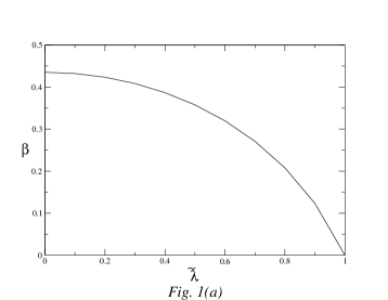
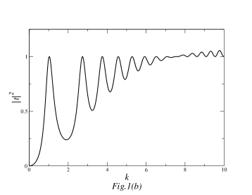
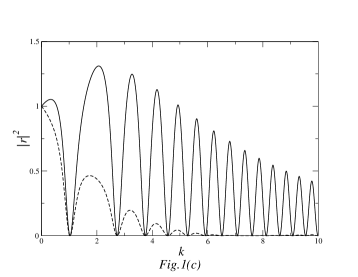
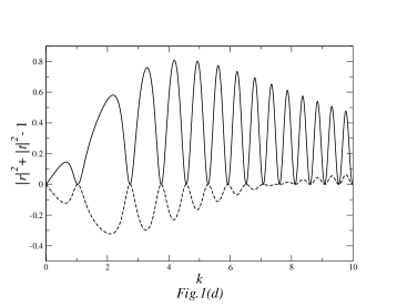
Figure 1: The figures above are for Model-I. The solid lines are for left incident beam and the dotted ones are for right incidence. 1(a): Variation of binding energy $(\beta=\sqrt{\frac{2mB}{\hbar^{2}}})$ with the strength of the imaginary part $(\tilde{\lambda}=\frac{2m\lambda}{\hbar^{2}})$ of the potential. Here we have taken $\frac{2mV_{0}}{\hbar^{2}}=1$ and $a=1$. 1(b): Variation of transmission coefficient $(|t|^{2})$ with the wavenumber $(k)$ for left (or right) incident beam. 1(c): Variation of reflection coefficient $(|r|^{2})$ with the wavenumber $(k)$ for left (or right) incident beam. 1(d): Variation of the deviation from unitarity $(|r|^{2}+|t|^{2}-1)$ with the wavenumber $(k)$ for left (or right) incident beam.

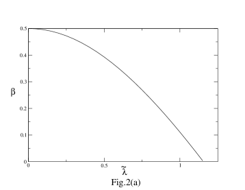
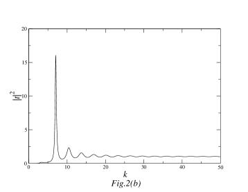
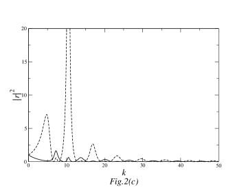
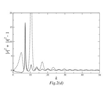
Figure 2: The figures above are for Model-II. The solid lines are for left incident beam and the dotted ones are for right incidence. 2(a): Variation of binding energy $(\beta=\sqrt{\frac{2mB}{\hbar^{2}}})$ with the strength of the imaginary part $(\tilde{\lambda}=\frac{2m\lambda}{\hbar^{2}})$ of the potential. Here we have taken $\frac{2mv_{0}}{\hbar^{2}}=1$ and range $a=1$. 2(b): Variation of transmission coefficient $(|t|^{2})$ with the wavenumber $(k)$ for left (or right) incident beam. 2(c): Variation of reflection coefficient $(|r|^{2})$ with the wavenumber $(k)$ for left (or right) incident beam. 2(d): Variation of the deviation from unitarity $(|r|^{2}+|t|^{2}-1)$ with the wavenumber $(k)$ for left (or right) incident beam.

For concreteness consider values of the potential parameters to be range $a=10$, real part of potential given by $\frac{2mV_{0}}{\hbar^{2}}=100$ and the strength of the imaginary part by $\frac{2m\lambda}{\hbar^{2}}=5$. We depict the energy variation of the transmission coefficient (which is the same for left and right incident beams) as a function of the wave number $k$ in $Fig.1(b)$. For the same potential the reflection coefficients for right and left incident beams are depicted in $Fig.1(c)$. The quantity ${{|}r{|}}^{2}+{{|}t{|}}^{2}$ which is equal to unity for real potentials will now depart from that value because of the imaginary part and this is a measure of the extent of inelasticity. Accordingly we plot ${{|}r{|}}^{2}+{{|}t{|}}^{2}-1$ for both left and right incident beams in $Fig.1(d)$.

As a second example of a $P$-Pseudo Hermitian Hamiltonian we choose a system of a particle in one dimension governed by

$$H=\frac{p^{2}}{2m}-v_{0}\delta(x)+i\lambda[\delta(x-\frac{a}{2})-\delta(x+\frac{a}{2})].$$ (10)

Here again $H^{\dagger}=PHP^{-1}$ but unlike case I the imaginary part of the potential is not proportional to the derivative of the real part. Defining $\frac{2mv_{0}}{\hbar^{2}}=\tilde{\mu}$, $\frac{2m\lambda}{\hbar^{2}}=\tilde{\lambda}$ and $\frac{2mB}{\hbar^{2}}=\beta^{2}$ where $B$ is the binding energy, the eigenvalue condition obtained from the jump conditions for the wavefunction becomes

$$8\beta^{3}-4\tilde{\mu}\beta^{2}={\tilde{\lambda}}^{2}(1-e^{{-\beta}a})[\tilde{\mu}(1-e^{-{\beta}a})-2\beta(1+e^{{\beta}a})].$$ (11)

Disregarding the unphysical double root of this equation at $\beta=0$ this is solved numerically and the variation of the binding energy is shown as a function of the strength of the imaginary part of the potential in $Fig.(2a)$ where we have for illustration chosen the real part to be given by $\tilde{\mu}=\frac{2mv_{0}}{\hbar^{2}}=1$ and the range $a=1$. It may again be noted that there exists no bound state (in the usual meaning of the word) below a certain critical value $(\mu_{cr})$ of the real part. This may easily be found from the eigenvalue condition $[eq.(9)]$ by putting its non-trivial root equal to zero and this leads to

$$\mu_{cr}=\frac{4{\tilde{\lambda}}^{2}a}{4+{\tilde{\lambda}}^{2}a^{2}}.$$ (12)

The transmission and reflection amplitudes for model-II are given by

$$t_{L}=t_{R}={1\over{(1-i\frac{\tilde{\mu}}{2k})+(\frac{\tilde{\lambda}}{2k})^{2}[-(1-i\frac{\tilde{\mu}}{2k})-i\frac{\tilde{\mu}}{k}e^{ika}+(1+i\frac{\tilde{\mu}}{2k})e^{2ika}]}},$$ (13)

$$r_{L}={i\frac{\tilde{\mu}}{2k}(1-\frac{\tilde{\lambda}}{k}+\frac{{\tilde{\lambda}}^{2}}{2{k}^{2}})+(1-\frac{\tilde{\lambda}}{2k})[(1+i\frac{\tilde{\mu}}{2k})\frac{\tilde{\lambda}}{2k}e^{ika}-c.c.]\over{(1-i\frac{\tilde{\mu}}{2k})+(\frac{\tilde{\lambda}}{2k})^{2}[-(1-i\frac{\tilde{\mu}}{2k})-i\frac{\tilde{\mu}}{k}e^{ika}+(1+i\frac{\tilde{\mu}}{2k})e^{2ika}]}},$$ (14)

$$r_{R}={i\frac{\tilde{\mu}}{2k}(1+\frac{\tilde{\lambda}}{k}+\frac{{\tilde{\lambda}}^{2}}{2{k}^{2}})-(1+\frac{\tilde{\lambda}}{2k})[(1+i\frac{\tilde{\mu}}{2k})\frac{\tilde{\lambda}}{2k}e^{ika}-c.c.]\over{(1-i\frac{\tilde{\mu}}{2k})+(\frac{\tilde{\lambda}}{2k})^{2}[-(1-i\frac{\tilde{\mu}}{2k})-i\frac{\tilde{\mu}}{k}e^{ika}+(1+i\frac{\tilde{\mu}}{2k})e^{2ika}]}},$$ (15)

where $c.c.$ stands for the complex conjugate of the preceeding term in the braces.

The reflection and transmission coefficients for left and right incident beams for this model and the departure from elastic unitarity are shown through $Fig.(2b)$ to $(2d)$. For both the models considered it can be easily seen that the condition for poles of the reflection and transmission amplitudes is exactly the equation for the binding energies, and thus the analytic structure in the energy ($k^{2}$) plane of these amplitudes shows bound state poles. They also have a cut along the real axis corresponding to a branch point at $k^{2}=0$ but the discontinuity across the cut is provided by inelastic unitarity arising from the imaginary part of the potential.

Thus we have discussed pseudo-Hermitian Hamiltonians in the context of one dimensional complex optical potentials and have shown that the energy eigenvalues are real for the strength of the imaginary part less than a critical value above which we obtain a complex conjugate pair of eigenvalues which create some difficulties in their interpretation. We also discuss transmission and reflection from such complex barriers and show that the reflection coefficient for left incident particles is different from that due to those coming from the right. We believe it is important to gain experience working with such pseudo-Hermitian Hamiltonians as their full physical significance is not yet very clear.

We gratefully acknowledge help from discussions with Swarnali Bandopadhyay and Abhishek Choudhury.

References

• [1] C. M. Bender and S. Boettcher, Phys. Rev. Lett. 80, 5243 (1998).
• [2] F. M. Fernandez, R. Guardiola, J. Ros, and M. Znojil, J. Phys. A: Math. Gen 31, 10105 (1998).
• [3] F. Cannata, G. Junker, and J. Trost, Phys. Lett. A 246, 219 (1998).
• [4] C. M. Bender, S. Boettcher, and P. N. Meisenger, J. Math. Phys. 40, 2201 (1999).
• [5] C. M. Bender, G. V. Dunne, and P. N. Meisenger, Phys. Lett. A 252, 272 (1999).
• [6] C. M. Bender and G. V. Dunne, J. Math. Phys. 40, 4616 (1999).
• [7] A. A. Andrianov, M. V. Ioffe, F. Cannata, and J. P. Dedonder, Int. J. Mod. Phys. A 14, 2675 (1999).
• [8] C. M. Bender, S. Boettcher, and V. M. Savage, J. Math. Phys. 41, 6381 (2000).
• [9] G. A. Mezincescu, J. Phys. A: Math. Gen 33, 4911 (2000).
• [10] E. Delabaere and D. T. Trinh, J. Phys. A: Math. Gen 33, 8771 (2000).
• [11] B. Bagchi and R. Roychoudhury, J. Phys. A: Math. Gen 33, L1-L3 (2000).
• [12] A. Khare and B. P. Mandal, Phys. Lett. A 272, 53 (2000).
• [13] B. Bagchi, F. Cannata, and C. Quesne, Phys. Lett. A 269, 79 (2000) .
• [14] M. Znojil, F. Cannata, B. Bagchi, and R. Roychoudhury, Phys. Lett. B 483, 284 (2000).
• [15] M. Znojil and M. Tater, J. Phys. A: Math. Gen 34, 1793 (2001).
• [16] C. M. Bender, G. V. Dunne, P. N. Meisenger, and M. Simsek, Phys. Lett. A 281, 311 (2001).
• [17] F. Cannata, M. Ioffe, R. Roychoudhury, and P. Roy, Phys. Lett. A 281, 305 (2001).
• [18] C. M. Bender, M. Berry, P. N. Meisenger, V. M. Savage, and M. Simsek, J. Phys. A: Math. Gen 34, L31 (2001).
• [19] P. Dorey, C. Dunning, and R. Tateo, β€˜Supersymmetry and the spontaneous breakdown of PT symmetry,’ LANL Archives: hep-th/0104119.
• [20] M. Znojil, β€˜PT-symmetrized supersymmetric quantum mechanics,’ LANL Archives: hep-th/0101038.
• [21] M. Znojil, β€˜Conservation of pseudo-norm in PT symmetric quantum mechanics,’ LANL Archives: math-ph/0104012.
• [22] G. S. Japaridze, β€˜Space of state vectors in PT symmetrized quantum mechanics,’ LANL Archives: quant-ph/0104077.
• [23] R. Kretschmer and L. Szymanowski,β€˜The interpretation of quantum- mechanical models with non-Hermitian Hamiltonians and real spectra,’ LANL Archives: quant-ph/0105054.
• [24] Ali Mostafazadeh, arXiv:math-ph/0107001.
• [25] M.A. Preston, Physics of the Nucleus (Addison-Wesley Publishing Company, Reading, 1965) pp 545.
• [26] B. Bagchi and C. Quesne, Phys. Lett. A 273 (2000) 285.
• [27] Z. Ahmed, Phys. Lett. A 290 (2001) 19.
• [28] Mostafazadeh, arXiv:math-ph/0110016.
• [29] A.S. Davydov, Quantum Mechanics, (Pergamon Press, Oxford, 1965) pp 513.