Implementation of dense coding using the generalized Grover’s algorithm

1.Introduction

Dense coding was proposed by Bennett, and Wiesner in 1992 [1]. It has been implemented in experiments [2, 3]. Utilizing entanglement properties, dense coding can transmit more than one bit of information by manipulating only one of the two particles in an Einstein-Podolsky-Rosen (EPR) state. Using the four EPR states, 2 bits of information can be transmitted in the following quantum communication scheme. Initially, Alice and Bob each obtain one particle in a starting EPR state. Bob manipulates his particle via one of four unitary operators so as to put the two-particle system into one of the four EPR states and then return the treated particle to Alice. Since the four manipulations result in the four EPR states, 2 bits of information can be sent from Bob to Alice. By determining the EPR state, Alice can read the encoded information. K. Shimizu et al proposed a scheme for enhancing the information capacity using a new degree of freedom [4]. In fact, the entangled states used in dense coding are not confined within the EPR states. The other entangled states, such as the superpositions of two EPR states, can also be used in dense coding. The generalized Grover’s algorithm is used to prepare the starting EPR state, and its inversion is used to determine the entangled state in decoding measurement.

In our previous work, we have synthesized EPR states using the generalized Grover’s algorithm and demonstrated the experimental results using nuclear magnetic resonance (NMR) [5]. In this paper, we will implement dense coding using the algorithm and demonstrate the scheme using NMR.

2.Synthesizing the superpositions of EPR states

For convenience, the four EPR states are denoted by $|\psi_{1}>=(|\uparrow\uparrow>+|\downarrow\downarrow>)/\sqrt{2}$, $|\psi_{2}>=(|\uparrow\uparrow>-|\downarrow\downarrow>)/\sqrt{2}$, $|\psi_{3}>=(|\uparrow\downarrow>+|\downarrow\uparrow>)/\sqrt{2}$, and $|\psi_{4}>=(|\uparrow\downarrow>-|\downarrow\uparrow>)/\sqrt{2}$, where $|\uparrow>$ and $|\downarrow>$ are the two spin states of a spin 1/2 particle. $|\psi_{1}>$, $|\psi_{2}>$, $|\psi_{3}>$, $|\psi_{4}>$ are a complete orthonormal set, and arbitrary state of the two-particle system can be expanded in terms of them. For an example, $|\uparrow\uparrow>=(|\psi_{1}>+|\psi_{2}>)/\sqrt{2}$.

A.Manipulation of one particle in EPR states

The manipulation of particle 2 is chosen as $R_{y}^{2}(\theta)=e^{i\theta I_{y}^{2}}$, which is expressed by

$$R_{y}^{2}(\theta)=\left(\begin{array}[]{cc}\cos(\theta/2)&\sin(\theta/2)\\ -\sin(\theta/2)&\cos(\theta/2)\end{array}\right),$$ (1)

where $I_{y}^{2}$ denotes the matrix for $y$ component of the angular momentum of the spin, with 2 specifying the affected particle and by setting $\hbar=1$. For particle 2, $R_{y}^{2}(\theta)$ transforms its states $|\uparrow>$ and $|\downarrow>$ to the superpositions described by

$$R_{y}^{2}(\theta)|\uparrow>=|\uparrow>\cos(\theta/2)-|\downarrow>\sin(\theta/2),$$ (2)

$$R_{y}^{2}(\theta)|\downarrow>=|\uparrow>\sin(\theta/2)+|\downarrow>\cos(\theta/2).$$ (3)

Using these two equations, $R_{y}^{2}(\theta)$ transforms the four EPR states into the superpositions of EPR states, which are expressed by

$$R_{y}^{2}(\theta)|\psi_{1}>=|\psi_{1}>\cos(\theta/2)-|\psi_{4}>\sin(\theta/2),$$ (4)

$$R_{y}^{2}(\theta)|\psi_{2}>=|\psi_{2}>\cos(\theta/2)-|\psi_{3}>\sin(\theta/2),$$ (5)

$$R_{y}^{2}(\theta)|\psi_{3}>=|\psi_{3}>\cos(\theta/2)+|\psi_{2}>\sin(\theta/2),$$ (6)

$$R_{y}^{2}(\theta)|\psi_{4}>=|\psi_{4}>\cos(\theta/2)+|\psi_{1}>\sin(\theta/2).$$ (7)

$R_{y}^{2}(\theta)$ causes rotations of the EPR states which are shown in Fig.1, where the black vectors denote the new states after rotations. In Fig.1(a), for example, $R_{y}^{2}(\theta)$ rotates $|\psi_{1}>$, denoted by the horizontal vector, by $-\theta/2$ radians in the two-dimensional vector space spanned by $|\psi_{1}>$ and $|\psi_{4}>$. Obviously, after the rotation, each EPR state is transformed to a superposition of two EPR states. One should note that the superposition is still the maximally entangled state.

Similarly, if the manipulation is chosen as $R_{x}^{2}(\theta)=e^{i\theta I_{x}^{2}}$, one obtains that $R_{x}^{2}(\theta)|\psi_{1}>=|\psi_{1}>\cos(\theta/2)+i|\psi_{3}>\sin(\theta/2)$, $R_{x}^{2}(\theta)|\psi_{2}>=|\psi_{2}>\cos(\theta/2)+i|\psi_{4}>\sin(\theta/2)$, $R_{x}^{2}(\theta)|\psi_{3}>=|\psi_{3}>\cos(\theta/2)+i|\psi_{1}>\sin(\theta/2)$, and $R_{x}^{2}(\theta)|\psi_{4}>=|\psi_{4}>\cos(\theta/2)+i|\psi_{2}>\sin(\theta/2)$. $R_{x}^{2}(\theta)$ also causes rotations of the EPR states. For example, it rotates $|\psi_{1}>$ by $\theta/2$ radians in the space spanned by $|\psi_{1}>$ and $i|\psi_{3}>$.

B.The generalized Grover’s algorithm

For a two-qubit system, the generalized Grover’s algorithm can be described as follows [6]. The unitary operator $U$ is chosen as $U=R_{y}^{1}(\varphi_{1})R_{y}^{2}(\varphi_{2})$, which is represented as

$$U=\left(\begin{array}[]{cccc}c_{1}c_{2}&c_{1}s_{2}&s_{1}c_{2}&s_{1}s_{2}\\ -c_{1}s_{2}&c_{1}c_{2}&-s_{1}s_{2}&s_{1}c_{2}\\ -s_{1}c_{2}&-s_{1}s_{2}&c_{1}c_{2}&c_{1}s_{2}\\ s_{1}s_{2}&-s_{1}c_{2}&-c_{1}s_{2}&c_{1}c_{2}\end{array}\right),$$ (8)

where $c_{k}(k=1,2)$ and $s_{k}$ are defined as $c_{k}\equiv cos(\varphi_{k}/2)$, and $s_{k}\equiv sin(\varphi_{k}/2)$. The basis states are arrayed as $|\uparrow\uparrow>$, $|\uparrow\downarrow>$, $|\downarrow\uparrow>$, $|\downarrow\downarrow>$. The conditional sign flip operators for $|\uparrow\uparrow>$ and $|\downarrow\downarrow>$, and for $|\uparrow\downarrow>$ and $|\downarrow\uparrow>$ can be chosen as the same form represented as

$$I_{t}=\left(\begin{array}[]{cccc}1&0&0&0\\ 0&-1&0&0\\ 0&0&-1&0\\ 0&0&0&1\end{array}\right).$$ (9)

If the predefined basis state is chosen as $|s>=|\uparrow\uparrow>$, the condition phase shift is represented as

$$I_{s}=\left(\begin{array}[]{cccc}-1&0&0&0\\ 0&1&0&0\\ 0&0&1&0\\ 0&0&0&1\end{array}\right).$$ (10)

A composite operator $G$ is defined as $G\equiv-UI_{s}U^{-1}I_{t}U$. When $U$ is chosen as $U_{1}=R_{y}^{1}(\pi/4)R_{y}^{2}(3\pi/4)$, $U_{2}=R_{y}^{1}(\pi/4)R_{y}^{2}(-3\pi/4)$, $U_{3}=R_{y}^{1}(\pi/4)R_{y}^{2}(\pi/4)$, and $U_{4}=R_{y}^{1}(\pi/4)R_{y}^{2}(-\pi/4)$, $G$ is represented as $G_{j}(j=1,2,3,4)=-U_{j}I_{s}U^{-1}_{j}I_{t}U_{j}$, which are expressed by

$$G_{1}=\frac{1}{2}\left(\begin{array}[]{cccc}-\sqrt{2}&-1&-1&0\\ 0&-1&1&-\sqrt{2}\\ 0&-1&1&\sqrt{2}\\ -\sqrt{2}&1&1&0\end{array}\right),$$ (11)

$$G_{2}=\frac{1}{2}\left(\begin{array}[]{cccc}-\sqrt{2}&1&-1&0\\ 0&-1&-1&-\sqrt{2}\\ 0&1&1&-\sqrt{2}\\ \sqrt{2}&1&-1&0\end{array}\right),$$ (12)

$$G_{3}=\frac{1}{2}\left(\begin{array}[]{cccc}0&1&1&\sqrt{2}\\ -\sqrt{2}&1&-1&0\\ -\sqrt{2}&-1&1&0\\ 0&1&1&-\sqrt{2}\end{array}\right),$$ (13)

$$G_{4}=\frac{1}{2}\left(\begin{array}[]{cccc}0&-1&1&-\sqrt{2}\\ \sqrt{2}&1&1&0\\ -\sqrt{2}&1&1&0\\ 0&1&-1&-\sqrt{2}\end{array}\right).$$ (14)

$G_{j}$ transform $|\uparrow\uparrow>$ to the four EPR states, where the initialization step is $U_{j}|\uparrow\uparrow>$ [5]. We apply $G_{j}$ to other basis states, i.e., the initial distribution of marked and unmarked states is changed [7], and obtain some useful results. If $G_{j}$ is applied to $|\downarrow\downarrow>$, the initialization step is $U_{j}|\downarrow\downarrow>$, and the results are also the four EPR states. However, $G_{j}$ transform $|\uparrow\downarrow>$ and $|\downarrow\uparrow>$ to the superpositions of EPR states. If $G=G_{2}$, one obtains

$$G_{2}|\uparrow\uparrow>=-|\psi_{2}>,$$ (15)

$$G_{2}|\downarrow\downarrow>=-|\psi_{3}>,$$ (16)

$$G_{2}|\uparrow\downarrow>=(|\psi_{1}>-|\psi_{4}>)/\sqrt{2},$$ (17)

$$G_{2}|\downarrow\uparrow>=(-|\psi_{1}>-|\psi_{4}>)/\sqrt{2},$$ (18)

using Eq. (12). Table 1 shows the results of the applications of $G_{j}$ to various basis states. In Table 1, the top row lists the basis states, the left column lists $G_{j}$, and the others are results, in which the irrelevant overall phase factors can be ignored. The superpositions of EPR states in Table 1 can be obtained through rotating EPR states using Eqs.(4)-(7) by setting $\theta=\pi/2$ or $-\pi/2$. For example, one can obtain Eqs.(17) and (18) from Eq.(4), by setting $\theta=\pi/2$ and $-\pi/2$, respectively.

TABLE 1. Results of the applications of $G_{j}(j=1,2,3,4)$ to various basis states.

	$|\uparrow\uparrow>$	$|\uparrow\downarrow>$	$|\downarrow\uparrow>$	$|\downarrow\downarrow>$
$G_{1}$	-$|\psi_{1}>$	(-$|\psi_{2}>$-$|\psi_{3}>$)/$\sqrt{2}$	(-$|\psi_{2}>$+$|\psi_{3}>$)/$\sqrt{2}$	-$|\psi_{4}>$
$G_{2}$	-$|\psi_{2}>$	($|\psi_{1}>$-$|\psi_{4}>$)/$\sqrt{2}$	(-$|\psi_{1}>$-$|\psi_{4}>$)/$\sqrt{2}$	-$|\psi_{3}>$
$G_{3}$	-$|\psi_{3}>$	($|\psi_{1}>$+$|\psi_{4}>$)/$\sqrt{2}$	($|\psi_{1}>$-$|\psi_{4}>$)/$\sqrt{2}$	$|\psi_{2}>$
$G_{4}$	$|\psi_{4}>$	(-$|\psi_{2}>$+$|\psi_{3}>$)/$\sqrt{2}$	($|\psi_{2}>$+$|\psi_{3}>$)/$\sqrt{2}$	-$|\psi_{1}>$

Because all the operators in $G$ are reversible, one can obtain $G^{-1}=-U^{-1}I_{t}UI_{s}U^{-1}$, using $I_{t}^{-1}=I_{t}$, and $I_{s}^{-1}=I_{s}$. $G^{-1}_{j}$ transform the results in Table 1 to the corresponding basis states. For example, $G_{3}^{-1}(-|\psi_{3}>)=|\uparrow\uparrow>$, $G_{3}^{-1}(|\psi_{1}>+|\psi_{4}>)/\sqrt{2}=|\uparrow\downarrow>$, $G_{3}^{-1}(|\psi_{1}>-|\psi_{4}>)/\sqrt{2}=|\downarrow\uparrow>$, and $G_{3}^{-1}|\psi_{2}>=|\downarrow\downarrow>$.

Similarly, when $U$ is chosen as $U_{1}=R_{x}^{1}(\pi/4)R_{x}^{2}(-3\pi/4)$, $U_{2}=R_{x}^{1}(\pi/4)R_{x}^{2}(3\pi/4)$, $U_{3}=R_{x}^{1}(\pi/4)R_{x}^{2}(\pi/4)$, and $U_{4}=R_{x}^{1}(\pi/4)R_{x}^{2}(-\pi/4)$, $G_{j}$ transform various basis states to the EPR states and the superpositions of EPR states. The superpositions can also be obtained through rotating the EPR states if the manipulation of particle 2 is chosen as $R_{x}^{2}(\theta)$. For example, if $U$ is chosen as $U_{1}=R_{x}^{1}(\pi/4)R_{x}^{2}(-3\pi/4)$, $G_{1}$ transforms $|\uparrow\uparrow>$ to $|\psi_{1}>$, $|\downarrow\downarrow>$ to $|\psi_{3}>$, $|\uparrow\downarrow>$ to $(|\psi_{2}>+i|\psi_{4}>)/\sqrt{2}$, and $|\downarrow\uparrow>$ to $(|\psi_{2}>-i|\psi_{4}>)/\sqrt{2}$, in which the two superpositions can be obtained by $R_{x}^{2}(\pi/2)|\psi_{2}>$ and $R_{x}^{2}(-\pi/2)|\psi_{2}>$, respectively.

3.Scheme of dense coding using the generalized Grover’s algorithm

The scheme is shown in Fig. 2, where 1 and 2 denote two quantum systems (qubits) with two states $|\uparrow>$ and $|\downarrow>$, and $|xy>$ denotes the output basis states. $G$ denotes the operation used to synthesize the starting EPR state using the generalized Grover’s algorithm. $V$ denotes one out of four manipulations of qubit 2 so that the two qubit system lies in one of four entangled states, including two EPR states and two superpositions of EPR states. The four manipulations are represented as $V_{1}=I$ (identity manipulation, i.e., nothing being done), $V_{2}=R_{y}^{2}(-\pi/2)\sigma_{x}=-R_{y}^{2}(\pi/2)\sigma_{z}$, $V_{3}=R_{y}^{2}(\pi/2)\sigma_{x}=R_{y}^{2}(-\pi/2)\sigma_{z}$, and $V_{4}=i\sigma_{y}$, where $\sigma_{x}$, $\sigma_{y}$ and $\sigma_{z}$ are $x$, $y$ and $z$ components of Pauli operator, and $\sigma_{x}=-iR_{x}(\pi)$, $\sigma_{y}=-iR_{y}(\pi)$, and $\sigma_{z}=-iR_{z}(\pi)=-ie^{i\pi I_{z}}$. $G^{-1}$ denotes the inversion of $G$, and it implements the decoding measurement of the whole system. $G^{-1}$ transforms the entangled state to the corresponding output state, by which Alice reads the encoded information. In the scheme, two bits of information are transmitted.

Now, we discuss an example. Let $|\psi_{2}>$ be the starting EPR state by setting $G=G_{2}$. $V_{1}$, $V_{2}$, $V_{3}$, and $V_{4}$ transform $|\psi_{2}>$ to $|\psi_{2}>$, $(|\psi_{1}>-|\psi_{4}>)/\sqrt{2}$, $(|\psi_{1}>+|\psi_{4}>)/\sqrt{2}$, and $|\psi_{3}>$, respectively. After the application of $G_{2}^{-1}$, the corresponding output states $|\uparrow\uparrow>$, $|\uparrow\downarrow>$, $|\downarrow\uparrow>$, and $|\downarrow\downarrow>$ are obtained, using the results in Table 1. Table 2 shows the correspondence between the starting EPR states and the output states. In Table 2, the top row lists the starting EPR states, the left column lists the four manipulations in dense coding, and the others are the output states.

TABLE 2. Correspondence between the starting EPR states and the output basis states.

	$|\psi_{1}>$	$|\psi_{2}>$	$|\psi_{3}>$	$|\psi_{4}>$
$V_{1}$	$|\uparrow\uparrow>$	$|\uparrow\uparrow>$	$|\uparrow\uparrow>$	$|\uparrow\uparrow>$
$V_{2}$	$|\downarrow\uparrow>$	$|\uparrow\downarrow>$	$|\uparrow\downarrow>$	$|\downarrow\uparrow>$
$V_{3}$	$|\uparrow\downarrow>$	$|\downarrow\uparrow>$	$|\downarrow\uparrow>$	$|\uparrow\downarrow>$
$V_{4}$	$|\downarrow\downarrow>$	$|\downarrow\downarrow>$	$|\downarrow\downarrow>$	$|\downarrow\downarrow>$

When the unitary operator $U$ in $G$ and $G^{-1}$ is chosen as $U=R_{x}^{1}(\pi/4)R_{x}^{2}(-3\pi/4)$, and $V$ is chosen as $V_{1}^{\prime}=I$, $V_{2}^{\prime}=R_{x}^{2}(\pi/2)\sigma_{z}$, $V_{3}^{\prime}=R_{x}^{2}(-\pi/2)\sigma_{z}$, $V_{4}^{\prime}=\sigma_{x}$, the scheme shown in Fig. 2 also carries out the dense coding. When the starting EPR state is $|\psi_{1}>$, for example, the output states are $|\uparrow\uparrow>$,$|\uparrow\downarrow>$, $|\downarrow\uparrow>$,$|\downarrow\downarrow>$, corresponding to the four manipulations, respectively. Compared with the previous scheme [2, 3], there are four new manipulations that are possible to be transmitted in the dense coding using the superpositions of EPR states. They are $V_{2}$, $V_{3}$,$V_{2}^{\prime}$, and $V_{3}^{\prime}$.

4. Demonstrating the scheme using NMR

Our experiments use a sample of carbon-13 labelled chloroform dissolved in d6-acetone. Data are taken at room temperature with a Bruker DRX 500 MHz spectrometer. The resonance frequencies $\nu_{1}=125.76$ MHz for ${}^{13}C$, and $\nu_{2}=500.13$ MHz for ${}^{1}H$. The coupling constant $J$ is measured to be 215 Hz. If the magnetic field is along $z$ axis, the Hamiltonian of this system is represented as [8]

$$H=-2\pi\nu_{1}I_{z}^{1}-2\pi\nu_{2}I_{z}^{2}+2\pi JI_{z}^{1}I_{z}^{2}.$$ (19)

In the rotating frame of spin $k$, the evolution caused by a radio-frequency (rf) pulse on resonance along $x$ or $-y$ axis is represented as $R_{x}^{k}(\varphi)$ or $R_{y}^{k}(-\varphi)$. The pulse used above is denoted by $[\varphi]_{x}^{k}$ or $[-\varphi]_{y}^{k}$. The coupled-spin evolution is denoted as

$$[\tau]=e^{-i2\pi J\tau I_{z}^{1}I_{z}^{2}}.$$ (20)

The pseudo-pure state is prepared by using spatial averaging [9]. The system in the equilibrium state is described by its deviation density matrix [10]

$$\rho_{eq}=\gamma_{1}I_{z}^{1}+\gamma_{2}I_{z}^{2},$$ (21)

where $\gamma_{k}$ denotes the gyromagnetic ratio of spin $k$. The following rf and gradient pulse sequence $[\alpha]_{x}^{2}-[grad]_{z}-[\pi/4]_{x}^{1}-1/4J-[\pi]_{x}^{1,2}-1/4J-[-\pi]_{x}^{1,2}-[-\pi/4]_{y}^{1}-[grad]_{z}$ transforms $\rho_{eq}$ to $\rho_{s}$ [11], which is represented as

$$\rho_{s}=I_{z}^{1}/2+I_{z}^{2}/2+I_{z}^{1}I_{z}^{2}.$$ (22)

$\rho_{s}$ is equivalent to $|s>$ [12]. The pulses are applied from left to right. $\alpha=\arccos(\gamma_{1}/2\gamma_{2})$, $[grad]_{z}$ denotes gradient pulse along $z$ axis, and the symbol $1/4J$ means that the system evolutes under the Hamiltonian $H$ for $1/4J$ time when pulses are switched off. $[\pi]_{x}^{1,2}$ denotes a nonselective pulse (hard pulse). The evolution caused by the pulse sequence $1/4J-[\pi]_{x}^{1,2}-1/4J-[-\pi]_{x}^{1,2}$ is equivalent to the coupled-spin evolution $[1/2J]$ described in Eq.(20) [13]. $[\pi]_{x}^{1,2}$ pulses are applied in pairs each of which take opposite phases in order to reduce the error accumulation causes by imperfect calibration of $\pi$-pulses [3].

we synthesize NMR analogs of EPR states (pseudo-EPR states) using the generalized Grover’s algorithm. Using Eq. (8), we realize $U_{1}$, $U_{2}$, $U_{3}$ and $U_{4}$ by $[\pi/4]_{y}^{1}-[3\pi/4]_{y}^{2}$, $[\pi/4]_{y}^{1}-[-3\pi/4]_{y}^{2}$, $[\pi/4]_{y}^{1,2}$, and $[\pi/4]_{y}^{1}-[-\pi/4]_{y}^{2}$, respectively. Obviously, $U_{1}^{-1}$, $U_{2}^{-1}$, $U_{3}^{-1}$, and $U_{4}^{-1}$ are realized by $[-\pi/4]_{y}^{1}-[-3\pi/4]_{y}^{2}$, $[-\pi/4]_{y}^{1}-[3\pi/4]_{y}^{2}$, $[-\pi/4]_{y}^{1,2}$, and $[-\pi/4]_{y}^{1}-[\pi/4]_{y}^{2}$. Because $I_{t}=I_{t}^{-1}=[1/J]$, $I_{t}$ and $I_{t}^{-1}$ are realized by $1/2J-[\pi]_{x}^{1,2}-1/2J-[-\pi]_{x}^{1,2}$. According to Ref. [14], $I_{s}$ and $I_{s}^{-1}$ are realized by $1/4J-[\pi]_{x}^{1,2}-1/4J-[-\pi]_{x}^{1,2}-[-\pi/2]_{y}^{1,2}-[-\pi/2]_{x}^{1,2}-[\pi/2]_{y}^{1,2}$. $V_{2}$, $V_{3}$ and $V_{4}$ are realized by $[\pi]_{x}^{2}-[-\pi/2]_{y}^{2}$, $[\pi]_{x}^{2}-[\pi/2]_{y}^{2}$, and $[\pi]_{y}^{2}$, respectively.

When the system lies in state $|\uparrow\uparrow>$, the carbon spectrum shown in Fig.3(a) and proton spectrum shown in Fig.3(e) are recorded through readout pulses $[\pi/2]_{y}^{1}$ and $[\pi/2]_{y}^{2}$, respectively. Through calibrating the phases of the signals in the two spectra, the two peaks are adjusted into absorption shapes. These two signals are used as reference signals of which phases are recorded to calibrate the phases of signals in other carbon spectra and proton spectra, respectively, so that the phases of the signals in the spectra are meaningful [15]. Pulses $[\pi]_{x}^{2}$, $[\pi]_{x}^{1}$ and $[\pi]_{x}^{1,2}$, transform $|\uparrow\uparrow>$ to $|\uparrow\downarrow>$, $|\downarrow\uparrow>$ and $|\downarrow\downarrow>$, respectively. Figs.3 (b-d) show the carbon spectra obtained by $[\pi/2]_{y}^{1}$, and Figs.3 (f-h) show the proton spectra obtained by $[\pi/2]_{y}^{2}$, when the system lies $|\uparrow\downarrow>$, $|\downarrow\uparrow>$ and $|\downarrow\downarrow>$, respectively.

The dense coding starts with $|\psi_{2}>$ by choosing $U=U_{2}$. The four manipulations are chosen as $V_{1}$, $V_{2}$, $V_{3}$, and $V_{4}$. Correspondingly, the carbon spectra are shown in Figs.4(a-d), obtained by $[\pi/2]_{y}^{1}$, and the proton spectra are shown in Figs.4(e-h), obtained by $[\pi/2]_{y}^{2}$. By comparing Figs.4 (a-d) with Figs.3 (a-d), and Figs.4 (e-h) with Figs.3 (e-h), respectively, we corroborate that the outputs are $|\uparrow\uparrow>$, $|\uparrow\downarrow>$, $|\downarrow\uparrow>$, and $|\downarrow\downarrow>$.

When $U=U_{1}$, $U_{3}$ or $U_{4}$, the dense coding starts with $|\psi_{1}>$, $|\psi_{3}>$ or $|\psi_{4}>$. The experimental results are also consistent with the theoretical predictions. When $U=U_{1}$, for example, manipulations $V_{2}$ and $V_{3}$ correspond to the carbon spectra shown in Figs.5(a-b), and the proton spectra shown in Figs.5(c-d). The readout pulses are still $[\pi/2]_{y}^{1}$ for the carbon spectra and $[\pi/2]_{y}^{2}$ for the proton spectra. By comparing Figs. 5(a-b) with Figs. 3(c) and (b), and Figs. 5(c-d) with Figs. 3(g) and (f), we corroborates that the outputs are $|\downarrow\uparrow>$ and $|\uparrow\downarrow>$.

4.Discussion

Two sets of messages can be transmitted by choosing two kinds of $U$ in decoding measurement. One kind takes form $R_{y}^{1}(\varphi_{1})R_{y}^{2}(\varphi_{2})$, such as $R_{y}^{1}(\pi/4)R_{y}^{2}(3\pi/4)$. The other kind takes form $R_{x}^{1}(\varphi_{1})R_{x}^{2}(\varphi_{2})$, such as $R_{x}^{1}(\pi/4)R_{x}^{2}(-3\pi/4)$. The two kinds of $U$ correspond the set of manipulations containing $I$, $R_{y}^{2}(\pi/2)\sigma_{z}$, $R_{y}^{2}(-\pi/2)\sigma_{z}$, and $i\sigma_{y}$, and the set containing $I$, $R_{x}^{2}(\pi/2)\sigma_{z}$, $R_{x}^{2}(-\pi/2)\sigma_{z}$, and $\sigma_{x}$, respectively. We propose an easy scheme to transmit the two sets of messages by introducing an ancilla two-state system, such as a classical bit or qubit. Alice and Bob can distinguish the two sets through the two states of the ancilla system. The starting EPR state is chosen as $|\psi_{1}>$, for example, by choosing $U=R_{y}^{1}(\pi/4)R_{y}^{2}(3\pi/4)$ or $R_{x}^{1}(\pi/4)R_{x}^{2}(-3\pi/4)$, noting that the two forms are equivalent in synthesizing $|\psi_{1}>$. Bob manipulates particle 2 via one of unitary operators in the two sets, and manipulates the ancilla system to denote which set the operator is in. Then he sends particle 2 and the ancilla system to Alice. Alice first determines the set in which the message lies by measuring the ancilla system. According to the measurement result, she chooses the proper kind of $U$ to read the encoding information through the decoding measurement as shown in Fig. 2. Because the ancilla system is independent of the two original particles in the entangled state, the scheme is easy to carry out.

5.Conlusion

We combine quantum communication with the quantum search algorithm, and propose a scheme of dense coding using the generalized Grover’s algorithm and its inversion. The experimental results verify our scheme. The superpositions of EPR states are used, and the messages possible to be transmitted increase.

This work was partly supported by the National Nature Science Foundation of China. We are also grateful to Professor Shouyong Pei of Beijing Normal University for his helpful discussions on the principle of quantum algorithm.

Figure Captions

1. Rotations of EPR states caused by manipulating particle 2, one EPR particle. The black vectors denote the states after manipulations, and they are superpositions of EPR states. The superpositions can be obtained by rotating the horizontal EPR states by $-\theta/2$ radians as shown in (a-b) and by $\theta/2$ radians as shown in (c-d).

2. Scheme of dense coding using the generalized Grover’s algorithm. $G$ denotes the operation carrying out the algorithm to synthesize the starting EPR state. $V$ denotes one of the four manipulations of particle 2. $G^{-1}$ , the inversion of $G$, implements the decoding measurement of the whole system.

3. Carbon spectra as shown in the left column obtained through selective readout pulse for ${}^{13}C$ denoted by $[\pi/2]_{y}^{1}$ and proton spectra as shown in the right column obtained through selective readout pulse for ${}^{1}H$ denoted by $[\pi/2]_{y}^{2}$ when the two-spin system lies in various pseudo-pure states. The amplitude has arbitrary units. Figures 2(a-d) and Figs. 2(e-h) correspond to states $|\uparrow\uparrow>$, $|\uparrow\downarrow>$, $|\downarrow\uparrow>$, and $|\downarrow\downarrow>$, respectively. The signals in Figs. 2(a) and (e) are used as reference signals to adjust other spectra.

4. Carbon spectra as shown in the left column obtained through $[\pi/2]_{y}^{1}$ and proton spectra as shown in the right column obtained through $[\pi/2]_{y}^{2}$ after the completion of dense coding when the starting pseudo-EPR state is $|\psi_{2}>$. Figs. 4(a-d) and Figs. 4(e-h) correspond to manipulations $V_{1}$, $V_{2}$, $V_{3}$, and $V_{4}$, respectively. Through comparing Figs. 4(a-d) with Figs. 3(a-d) and Figs. 4(e-h) with Figs. 3(e-h), one can corroborate that the corresponding four output states are $|\uparrow\uparrow>$, $|\uparrow\downarrow>$, $|\downarrow\uparrow>$, and $|\downarrow\downarrow>$.

5. Carbon spectra as shown in the left column obtained through $[\pi/2]_{y}^{1}$ and proton spectra as shown in the right column obtained through $[\pi/2]_{y}^{2}$ after the completion of dense coding when the starting pseudo-EPR state is $|\psi_{1}>$. Figs. 5(a-b) and Figs. 5(c-d) correspond to $V_{2}$ and $V_{3}$, respectively. Through comparing Figs. 5(a-b) with Figs. 3(c) and (b), and Figs. 5(c-d) with Figs. 3(g) and (f), one can corroborate that the two output states are $|\downarrow\uparrow>$ and $|\uparrow\downarrow>$, respectively.

1

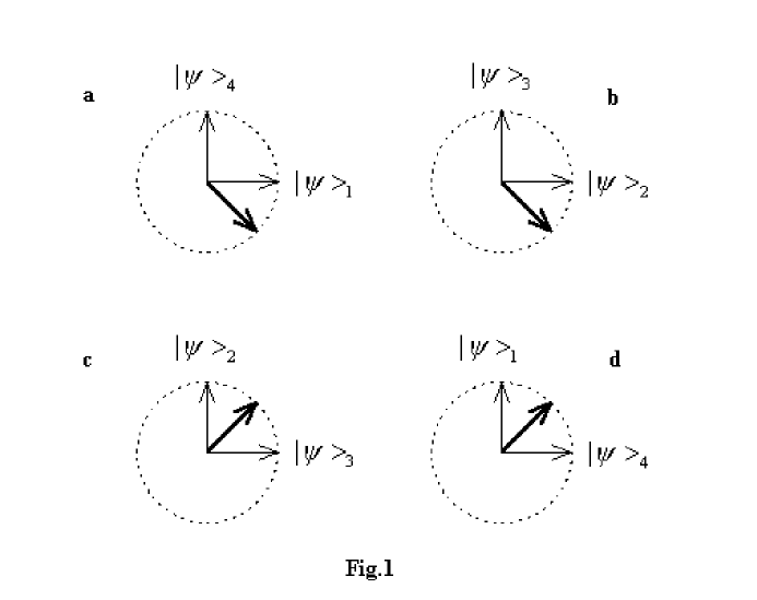
Figure 1:

2

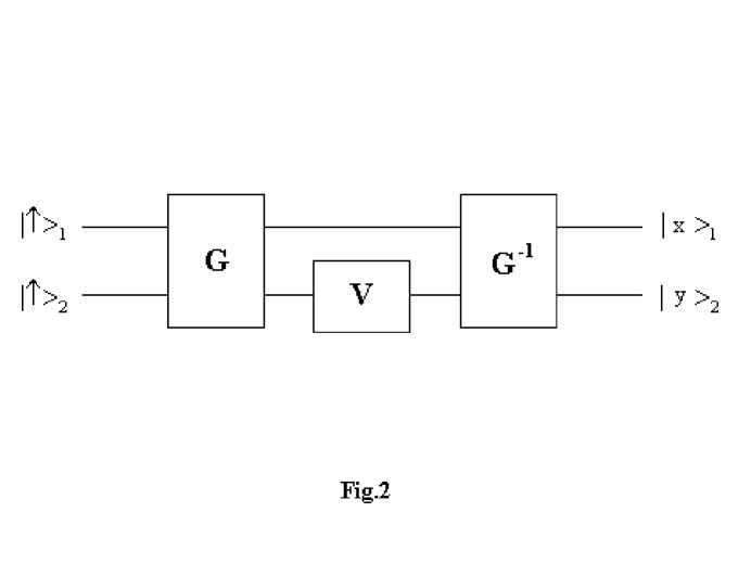
Figure 2:

3

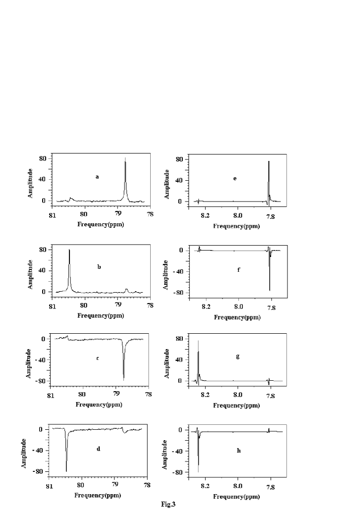
Figure 3:

4

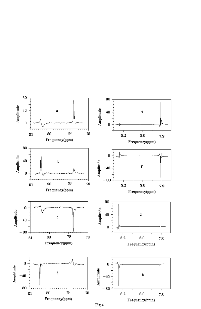
Figure 4:

5

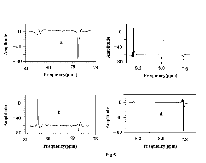
Figure 5:

References

- [1] C.H. Bennett, and S.J. Wiesner, Phys. Rev. Lett,69,2881(1992)
- [2] K. Mattle, H. Weinfurter, P.G. Kwiat, and A. Zeilinger, Phys. Rev. Lett, 76, 4656(1996)
- [3] X.-M. Fang, X.-W. Zhu, M. Feng, X.-A. Mao, and F.Du, Phys. Rev. A, 61,022307 (2000)
- [4] K. Shimizu, N. Imoto, and T. Mukai, Phys. Rev. A 59,1092(1999)
- [5] J.-F. Zhang, Z.-H. Lu, L. Shan, and Z.-W. Deng, Phys. Rev. A, Phys. Rev. A, 66, 0543xx(2002)(in pressing)
- [6] L.K. Grover, Phys. Rev. Lett, 80, 4329(1998)
- [7] E. Biham, O. Biham, D. Biron, M. Grassl, D.A. Lidar,and D. Shapira, Phys. Rev. A, 63, 012310(2000)
- [8] R.R. Ernst, G. bodenhausen and A. Wokaum, Principles of nuclear magnegtic resonance in one and two dimensions (Oxford University Press, New York, 1987)
- [9] D.G. Cory, M.D. Price, and T.F. Havel, Physica D. 120, 82(1998)
- [10] I. L.Chuang, N. Gershenfeld, M.G. Kubinec and D.W. Leung, Proc.R.Soc.Lond.A 454, 447 (1998)
- [11] J.-F. Zhang, Z.-H. Lu, L. Shan, and Z.-W. Deng, Phys. Rev. A, 65, 034301 (2002)
- [12] E.Knill, I. Chuang, and R. Laflamme, Phys. Rev. A 57, 3348 (1998)
- [13] N. Linden, . Kupe, and R. Freeman, Chem. Phys. Lett, 311, 321(1999)
- [14] I.L. Chuang, N. Gershenfeld, and M. Kubinec. Phys. Rev. Lett. 80,3408 (1998)
- [15] J. A. Jones, in The Physics of quantum Information, edited by D. Bouwmeester, A.Ekert, and A. Zeilinger. (Springer, Berlin Heidelberg, 2000) pp.177-189.