Geometric phase shift in quantum computation using superconducting nanocircuits: nonadiabatic effects

Quantum computation is now attracting increasing interest both theoretically and experimentally. So far, a number of systems have been proposed as potentially viable quantum computer models, including trapped ions, cavity quantum electrodynamics, nuclear magnetic resonce(NMR), etc [1]. In particular, a kind of solid state qubits using controllable low-capacitance Josephson juctions has been paid considerable attention[2, 3, 4, 5]. A two-qubit gate in many experimental implementations is the controlled phase shift, which may be achieved using either a conditional dynamic or geometric phase. A remarkable feature of the latter lies in that it depends only on the geometry of the path executed[6], and therefore provides a possibility to perform quantum gate operations by an intrinsically fault-tolerant way[7, 8].

Recently, several basic ideas of adiabatic geometric quantum computation by using NMR[8], superconducting nanocircuits[5] or trapped ions[9] were proposed. However, since some of the quantum gates are quite sensitive to perturbations of the phase factor of the computational basis states, control of the phase factor becomes an important issue for both hardware and software. Moreover, the adiabatic evolution appears to be quite special, and thus the nonadiabatic correction on the phase shift may need to be considered in some realistic systems as it may play a significant role in a whole process  [10, 11, 12]. In this paper, we focus on the nonadiabatic geometric phase in superconducting nanocircuits. We indicate that the adiabatic Berry’s phase, as well as the single qubit gate controlled by this phase, may hardly be implemented in the present experimental setup. On the other hand, since the 2-qubit operations are about $10^{2}$ times slower than the 1-bit operations[3], the conditional adiabatic phase is extremely difficult to be achieved. A serious disadvantange of the adiabatic conditional phase shift is that the adiabatic condition requires that the evolution time must be much longer than the typical operation time $\tau_{0}$ ($=\hbar/E_{J}$ with $E_{J}$ as the Josephson energy), which leads to an intrinsical time limitation on the operation of quantum gate. Therefore, a generalization to nonadiabatic cases is important in controlling the quantum gates. We find that the nonadiabatic geometric phase shift can also be used to achieve the phase shift in quantum gates.

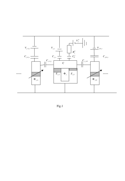
FIG. 1.: Schematic diagram of a quantum computer. The $j$-th qubit and its probe circuit are displayed in detail.

We first consider a single qubit using Josephson juctions described in Ref.[5] ( see the j-th qubit in Fig.1). The qubit consists of a superconducting electron box formed by an asymmetric SQUID with the Josephson coupling $E_{1}$ and $E_{2}$, pierced by a magnetic flux $\Phi$ and subject to an applied gate voltage $V_{x}=2en^{e}_{x}/C_{x}$ (here we omit the subscript $j$, and $2en^{e}_{x}$ is the offset charge). In the charging regime (where $E_{1,2}$ are much smaller than the charging energy $E_{ch}$) and at low temperatures, the system behaves as an artificial spin-$1/2$ particle in a magnetic field, and the effective Hamiltonian reads [13]

$$\hat{H}=-\frac{1}{2}{\bf B}\cdot\stackrel{{\scriptstyle\rightarrow}}{{\sigma}},$$ (1)

where $\sigma_{x,y,z}$ are Pauli matrices, and the fictitious field

$${\bf B}=\{E_{J}cos\alpha,-E_{J}sin\alpha,E_{ch}(1-2n^{e}_{x})\}$$ (2)

with $E_{J}=\sqrt{(E_{1}-E_{2})^{2}+4E_{1}E_{2}cos^{2}(\pi\Phi/\Phi_{0})}$, $tan\alpha=(E_{1}-E_{2})tan(\pi\Phi/\Phi_{0})/(E_{1}+E_{2})$, and $\Phi_{0}=h/2e$. In this qubit Hamiltonian, charging energy is equivalent to the $B_{z}$ field whereas the Josephson term determines the fields in the $xy$ plane. By changing $V_{x}$ and $\Phi$ the qubit Hamiltonian describes a curve in the parameter space $\{{\bf B}\}$. Therefore by adiabatically changing $\hat{H}$ around a circuit in $\{{\bf B}\}$, the eigenstates will accumulate a Berry’s phase $\gamma_{B}=\mp\Omega/2$, where the signs $\pm$ depend on whether the system is in the eigenstate aligned with or against the field[6]. The solid angle $\Omega$, which represents the magnetic field trajectory subtends at ${\bf B}=0$, is derived as

$$\Omega=\int_{0}^{\tau}\frac{B_{x}\partial_{t}B_{y}-B_{y}\partial_{t}B_{x}}{|{\bf B}|(B_{z}+|{\bf B}|)}dt,$$ (3)

under the condition ${\bf B}(\tau)={\bf B}(0)$.

However, the adiabatic evolution is quite special, and thus the generalization to nonadiabatic noncyclic cases is of significance. We now recall how to calculate the Pancharatnam phase. For a spin-$1/2$ particle subject to an arbitrary magnetic field, each spin state $|\psi\rangle=[e^{-i\varphi/2}cos(\theta/2),\ e^{i\varphi/2}sin(\theta/2)]^{T}$ may be mapped into a unit vector ${\bf n}=(sin\theta cos\varphi,sin\theta sin\varphi,cos\theta)$, with ${\bf n}\in$ a unit sphere $S^{2}$, via the relation ${\bf n}=\langle\psi|\stackrel{{\scriptstyle\rightarrow}}{{\sigma|}}\psi\rangle$, where $T$ represents the transposition of matrix. By changing the magnetic field, the evolution of spin state is a curve on $S^{2}$ from an initial state $(\theta_{i},\varphi_{i})$ to a final state $(\theta_{f},\varphi_{f})$, and the Pancharatnam phase accumulated in this evolution was found to be [11]

$$\gamma=-\frac{1}{2}\int_{C}(1-cos\theta)d\varphi+arctan\frac{sin(\varphi_{f}-\varphi_{i})}{cot\frac{\theta_{f}}{2}cot\frac{\theta_{i}}{2}+cos(\varphi_{f}-\varphi_{i})},$$ (4)

where $C$ is along the actual evolution curve on $S^{2}$, and is determined by the equation: $\partial_{t}{\bf n}(t)=-{\bf B}(t)\times{\bf n}(t)/\hbar$. This $\gamma$ phase recovers the Aharonov-Anandan (AA) phase (Berry’s phase) in a cyclic (adiabatic) evolution[11].

At this stage, we propose how to detect the nonadiabatic or adiabatic geometric phase in the charge qubit system. The system is prepared in the ground state of the Hamiltonian at $n^{e}_{x}=0$ and $\Phi=0$, and then changes to the fictitious field ${\bf B}(\Phi(t),n_{x}^{e}(t))$, which is a periodic function of time $t$ with the period $\tau$. We consider the process where a pair of orthogonal states $|\psi_{\pm}\rangle$ evolve cyclically(but not necessary adiabatically). This process can be realized in the present system. Noting that the adiabatic approximation is merely a sufficient but not necessary condition for the above cyclic evolution, we here focus on a nonadiabatic generalization. In this evolution, the initial state is given by

$$|\psi_{i}\rangle=a_{+}|\psi_{+}(\theta_{i},\varphi_{i})\rangle+a_{-}|\psi_{-}(\theta_{i},\varphi_{i})\rangle,$$

where

$$| \psi_{+}(\theta,\varphi)\rangle=[e^{-i\varphi/2}cos(\theta/2),\ e^{i\varphi/2}sin(\theta/2)]^{T},$$

$$| \psi_{-}(\theta,\varphi)\rangle=[-e^{-i\varphi/2}sin(\theta/2),\ e^{i\varphi/2}cos(\theta/2)]^{T},$$

$$a {}_{+}=cos[(\eta-\theta_{i})/2]cos\varphi_{i}/2-icos[(\eta+\theta_{i})/2]sin\varphi_{i}/2,$$

$$a {}_{-}=sin[(\eta-\theta_{i})/2]cos\varphi_{i}/2+isin[(\eta+\theta_{i})/2]sin\varphi_{i}/2,$$

with $tan\eta=E_{J}(\Phi=0)/E_{ch}$, $tan\theta_{i}=[E_{J}(t)/B_{z}(t)]|_{t=0}$, and $tan\varphi_{i}=[B_{y}(t)/B_{x}(t)]|_{t=0}$. A phase difference between $|\psi_{+/-}\rangle$ can be introduced by changing $\hat{H}$. The phases acquired in this way will have both geometrical and dynamical components. But the dynamical phase accumulated in the whole procedure may be removed[14], thus only the geometric phase remains. By taking into account the cyclic condition ${\bf n}(0)={\bf n}(\tau)$ for $|\psi_{\pm}\rangle$, the final state in this case is given by[15]

$$|\psi_{f}\rangle=a_{+}e^{i\gamma}|\psi_{+}(\theta_{i},\varphi_{i})\rangle+a_{-}e^{-i\gamma}|\psi_{-}(\theta_{i},\varphi_{i})\rangle,$$ (5)

where $\gamma$ can be calculated from Eq.(4). The contribution from the second term of Eq.(4) vanishes simply because ${\bf n}(0)={\bf n}(\tau)$. Thus the geometric phase considered here is the cyclic AA phase. The probability of measuring a charge $2e$ ($n=1$) in the box at the end of this procedure is derived as

$$P_{1}=|a_{+}sin\frac{\theta_{i}}{2}+a_{-}cos\frac{\theta_{i}}{2}e^{-2i\gamma}|^{2}.$$ (6)

This probability can be simplified to

$$P_{1}=[1-cos(\eta-\theta_{i})cos\theta_{i}+sin(\eta-\theta_{i})sin\theta_{i}cos2\gamma]/2.$$ (7)

when $\Phi(0)=0$. Note that Eq.(7) recovers $sin^{2}(\gamma)$ in Ref.[5] even in a nonadiabatic but cyclic evolution[16]. Thus the nonadiabatic phase may be determined by the probability of the charge state in the box at the end of this process. It is worth pointing out that the parameters $\eta$ and $\theta_{i}$ in Eq.(6)(or(7)) are fully determined by the experimentally controllable parameters $\Phi$ and $n_{x}^{e}$, as in the adiabatic Berry’s phase case [5].

It is remarkable that the probability obtained in Eq.(6)(or(7)) may be directly detected by the dc current through the probe junction $C_{b}^{j}$ under a finite bias voltage $V_{b}^{j}$[4]. Assume that we have achieved one SQUID qubit as well as the detector circuit, as shown in Fig.1. By changing $V_{jx}$ and $\Phi_{j}$ in time $[0,\tau]$, the system oscillates between $|0\rangle$ and $|1\rangle$, and the final state would be determined by the geometric phase. The measurable dc current through the probe junction formulates by the processes: $|1\rangle$ emits two electrons to the probe, while $|0\rangle$ does nothing. Consequently, the probability described by Eq.(6)(or (7)) as well as the geometric phase may be detected by the dc current.

The single qubit gate may be realized by this geometric phase. For example, it is straightforward to check that the unitary evolution operator defined by $|\psi_{f}\rangle=U^{sq}_{1}|\psi_{i}\rangle$, is given by

$$U_{1}^{sq}(\gamma)=\left(\begin{array}[]{ll}cos\gamma&isin\gamma\\ isin\gamma&cos\gamma\end{array}\right),$$ (8)

when $\theta_{i}=0$ and $\varphi_{i}=0$. Clearly, the operation depends on the geometric phase $\gamma$; $\gamma=\pi/2$ and $\gamma=\pi/4$ procduce a spin flip (NOT-operation) and an equal-weight superposition of spin states, respectively. On the other hand, the phase-flip gate $U_{2}^{sq}=exp(-2i\gamma|1\rangle\langle 1|)$ (up to an irrelevant over phase ) is derived by $\theta_{i}=0$ and $\varphi_{i}=0$. The noncommutable $U_{1}^{sq}$ and $U_{2}^{sq}$ gates are the two well-known universal gates for single-qubit operation. The Berry’s phase may be used to achieve intrinsical fault-tolerant quantum computation since it depends only on the evolution path in the parameter space. The nonadiabatic cyclic phase is also rather universal in a sense that it is the same for a infinite number of possible ways of motion along the curves in the projective Hilbert space[10]. Consequently, the nonadiabatic phase may also be used as a tool for some fault-tolerant quantum computation.

We now illustrate how to achieve the cyclic state for quantum gates in two processes. The parameters $(\Phi(t),n_{x}^{e}(t))$ in process I change as

$$(I)\left\{\begin{array}[]{ll}\{\frac{4\Phi_{m}t}{\tau},\frac{1}{2}\},&t\in[0,\frac{\tau}{4})\\ \{\Phi_{m},\frac{1}{2}+4(n_{xm}^{e}-\frac{1}{2})(\frac{t}{\tau}-\frac{1}{4})\},&t\in[\frac{\tau}{4},\frac{1\tau}{2})\\ \{-4\Phi_{m}t/\tau+3\Phi_{m},n_{xm}^{e}\},&t\in[\frac{1\tau}{2},\frac{3\tau}{4})\\ \{0,n_{xm}+4(\frac{1}{2}-n_{xm}^{e})(\frac{t}{\tau}-\frac{3}{4})\}.&t\in[\frac{3\tau}{4},\tau)\end{array}\right.$$ (9)

The path in the parameter space $\{{\bf B}\}$ swept out in this case is exactly the same as that proposed in Ref.[5], Since the evolution in this process is cyclic only under the adiabatic condition, we need to answer a key question: whether the adiabatic approximation is valid for the given parameters? As for process II , the parameters $(\Phi(t),n_{x}^{e}(t))$ change as

$$(II)\left\{\begin{array}[]{c}\Phi(t)=\frac{\Phi_{0}}{\pi}atan[\frac{E1+E2}{E1-E2}tan(\omega t)],\\ n^{e}_{x}(t)=\frac{1}{2}(1-\frac{E_{J}ctg\chi_{0}+\hbar\omega}{E_{ch}}).\end{array}\right.$$ (10)

The fictitious field described by Eq.(10) guarantees that the angle $\chi_{0}=arctan[E_{J}/(B_{z}(t)-\hbar\omega)]$ (and $n_{z}$) is time-independent. It is found that the state described by the vectors ${\bf n}(\chi_{0},-\omega t)$ in this process evolves cyclically with period $\tau=2\pi/\omega$ [17], and the AA phase for one cycle is given by $\gamma=\pi(1-cos\chi_{0})$, which may be used to achieve the mentioned single-qubit gates geometrically. For the present system, the dynamic phase can be removed by simply choosing $\omega=-4(E_{1}+E_{2})E_{k}[-4E_{1}E_{2}/(E_{1}-E_{2})^{2}]/\pi sin(2\chi_{0})$ with $E_{k}(x)$ the complete elliptic integral of the first kind.

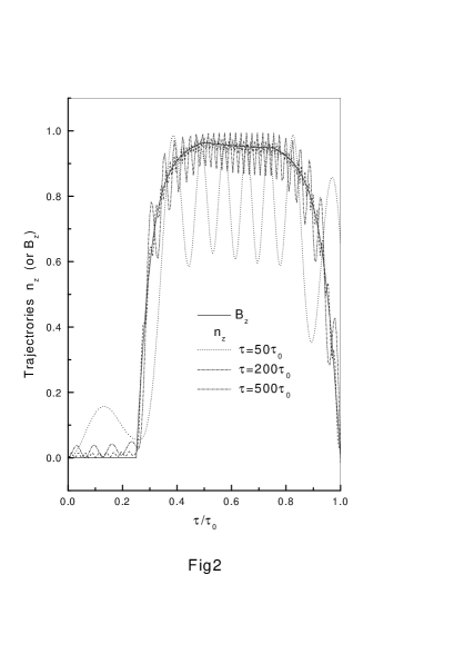
FIG. 2.: The trajectories $n_{z}$ and $\hat{B}_{z}$ versus time in process I for $\Phi_{m}=0.25$, $n^{e}_{xm}=0.20$, $E_{2}=4E_{1}=6.25\mu ev$, and $E_{ch}=5.0(E_{1}+E_{2})$.

The nonadiabatic effect should be important if $\tau$ is not short. We first consider the evolutions described by Eq.(9). Figure 2 shows $n_{z}(t)$ and $\hat{B}_{z}(t)=B_{z}(t)/|{\bf B}(t)|$ versus time, with the parameters being the same as those in Ref.[4]. The deviation of ${\bf n}(t)$ from $\hat{{\bf B}}(t)(={\bf B}(t)/|{\bf B}(t)|)$ indicates clearly whether or not the adiabatic approximation is valid because ${\bf n}(t)$ almost follows the trajectory of the magnetic field $\hat{{\bf B}}(t)$ under this approximation. It is seen from Fig.2 that the adiabatic approximation is satisfied in the first case when $\tau>500\tau_{0}$, where $\tau_{0}=\hbar/(E_{1}+E_{2})\sim 84ps$. The adiabatic condition for process II is in the same order of magnitude (see Fig.3). It is worth pointing out that the coherence time achieved in a single SQUID is merely about $30\sim 40\tau_{0}$[4], which is not long enough for the adiabatic evolution, implying that the adiabatic condition is not satisfied in the above two processes for realistic systems. But, fortunately, the nonadiabatic phase can be measured and used in achieving geometric quantum gates.

Conditional geometric phase accumulated in one sub-system evolution depends on the quantum state of another sub-system, which may be realized by coupling capacitively two asymmetric SQUIDS (see any neighboring pair of qubits in Fig.1.). If the coupling capacitance $C_{ij}$ is smaller than the others, the Hamiltonian reads

$$\hat{H}=\sum\limits_{i=1}^{N}\hat{H}_{i}+\sum\limits_{i=1}^{N-1}(\hat{H}_{i,i+1}+H.C.),$$ (11)

where $H_{i}$ refer to the uncoupled qubits defined in Eq.(1) and $\hat{H}_{i,i+1}=E_{i,i+1}(n^{e}_{i}-n^{e}_{x,i})(n^{e}_{i+1}-n^{e}_{x,i+1})$ with $E_{i,i+1}=E_{ch}C_{i,i+1}/C$[5]. The gate voltage and magnetic flux can be independently fixed for all qubits. We address firstly a two-qubit operation, e.g., $i$ and $j$ qubits are two neighbour qubits with the i-th as the control qubit and the j-th as the target qubit. The fictitious field on the target qubit is $[E_{J}(\Phi_{j})cos\alpha_{j},-E_{J}(\Phi_{j})sin\alpha_{j},B_{z}^{l}]$ with $B_{z}^{l}=E_{ch}(1-2n^{e}_{x,j})+E_{i,j}(n^{e}_{x,i}-l)$, where $l$ represent the control qubit state $0$ or $1$. Obviously, the geometric phase $\gamma_{j}$ for $j$-th qubit in decoupled case is different from $\gamma_{j}^{l}$ even the changeings of $(\Phi_{j},n^{e}_{x,j})$ are the same, where $\gamma_{j}^{l}$ is the geometric phase of the target qubit when the charge state of the control qubit is $l$. $\gamma_{j}^{l}$ may be directly derived from Eq.(4). It is worth to pointing out that the state described by the vector ${\bf n}(\chi^{l},-\omega t)$ with $\chi_{0}^{l}=arctan[E_{J}/(B_{z}^{l}-\hbar\omega)]$ is still a cyclic evolution, and may be used to achieve the two-qubit operation. In terms of the basis $\{|00\rangle,|01\rangle,|10\rangle,|11\rangle\}$, the unitary operator to describe the two-qubit gate is given by [5]

$$U_{(\gamma^{0}_{j},\gamma^{1}_{j})}=diag(e^{-i\gamma^{0}_{j}},e^{i\gamma^{0}_{j}},e^{-i\gamma^{1}_{j}},e^{i\gamma_{j}^{1}}).$$ (12)

The combination with single-bit operations allow us to perform the XOR gate. The unitary operation for XOR gate can be obtained by $U_{XOR}=\left[I\otimes U_{1}^{sq}(\pi/4)\right]U_{(0,\frac{3\pi}{2})}\left[I\otimes U_{1}^{sq}(\pi/4)\right]^{\dagger}$ with $I$ as a $2\times 2$ unit matrix. This XOR gate together with single qubit gates constitutes a universality: they are sufficient for all manipulations required for quantum computation [18]. Therefore, all the elements of quantum computation may be achievable by (nonadiabatic) geometric phase.

We now compute the geometric phases required by the spin flip operation ($\gamma=3\pi/2$) and NOT operation ($\gamma=3\pi/4$) accumulated in the second process. The comparison of the nonadiabatic geometric phase $\gamma$ with $\gamma_{a}$ is shown in Fig.3, where the $\gamma_{a}$ is the phase calculated under the adiabatic approximation. It is seen that the $\gamma_{a}$ deviates evidently from the $\gamma$ for $\tau<150\tau_{0}$. Thus the operation time required by the adiabatic condition in both processes I and II is in the same order of magnitude. The dynamic phases can be removed when $\tau\sim 3.57\tau_{0}$ for $\gamma=3\pi/2$ and $\tau\sim 4.12\tau_{0}$ for $\gamma=3\pi/4$, respecitively. Therefore, by accurately controlling the parameters $\Phi$ and $n_{x}^{e}$, we may control the state in the projective Hilbert space. It is striking that the present operation time for nonadiabatic geometric gates is much shorter than that with the adiabatic scheme. Note that the coherence time achieved in a single SQUID by current technology is about $30\sim 40\tau_{0}$[4], implying that tens of geometric NOT operation may be achieved experimentally. Therefore, the generalization of the adiabatic phase to the nonadiabatic case is of significance since the coherence time achieved in charge qubit in Josephson Junctions is short. Moreover, the large number qubits required for useful computation may be devised by a network similar to Fig.1.

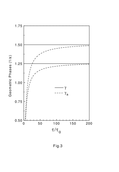
FIG. 3.: The comparison of adiabatic phases with nonadiabatic ones. The parameters are the same as those in Fig.2.

In conclusion, we study how to detect the nonadiabatic phase in superconducting nanocircuits, and the possibility to use the nonadiabatic phase as a tool to achieve the quantum computation.

We wish to acknowledge valuable discussions with Dr. L. M. Duan and Dr. X. B. Wang. This work was supported by the RGC grant of Hong Kong under Grant Nos. HKU7118/00P and HKU7114/02P, the Ministry of Science and Technology of China under Grant No. G1999064602, and the URC fund of HKU. S. L. Z. was supported in part by the SRF for ROCS, SEM, the NSF of Guangdong under Grant No. 021088, and the NNSF of China under Grant No. 10204008.

REFERENCES

- [1] J. I. Cirac and P. Zoller, Phys. Rev. Lett. 74, 4091 (1995); T. Pellizzari, S. A. Gardiner, J. I. Cirac, and P. Zoller, Phys. Rev. Lett. 75, 3788 (1995); N. A. Gershenfeld and I. L. Chuang, Science 275, 350 (1997).
- [2] A. Shnirman, G. Schön, and Z. Hermon, Phys. Rev. Lett. 79, 2371 (1997); D. V. Averin, Solid State Comm. 105, 659 (1998).
- [3] Y. Makhlin, G. Schön, and A. Shnirman, Nature, 398, 305 (1999); Rev. Mod. Phys. 73, 357 (2001).
- [4] Y. Nakamura, Yu. A. Pashkin, and J. S. Tsai, Nature 398, 786 (1999); Physica B 280, 405 (2000).
- [5] G. Falci, R. Fazio, G. M. Palma, J. Siewert, and V. Vedral, Nature 407, 355 (2000).
- [6] M. V. Berry, Proc. R. Soc. London A 392, 45 (1984).
- [7] P. Zanardi and M. Rasetti, Phys. Lett. A 264, 94 (1999).
- [8] J. A. Jones, V. Vedral, A. Ekert, and G. Castagnoli, Nature 403, 869 (2000).
- [9] L. M. Duan, J. I. Cirac, and P. Zoller, Science 292, 1695 (2001).
- [10] Y. Aharonov and J. Anandan, Phys. Rev. Lett. 58, 1593 (1987).
- [11] S. L. Zhu and Z. D. Wang, Phys. Rev. Lett. 85, 1076 (2000); S. L. Zhu, Z. D. Wang, and Y. D. Zhang, Phys. Rev. B. 61, 1142 (2000); Z. D. Wang and S. L. Zhu, Phys. Rev. B 60, 10668 (1999).
- [12] S. L. Zhu and Z. D. Wang, Phys. Rev. Lett. 89, 097902 (2002).
- [13] D. V. Averin and K. K. Likharev, in B. L. Altshuler, P. A. Lee, and R. A. Webb, Mesoscopic Phenomena in Solids (Elsevier, New York, 1991), p213.
- [14] A useful method is to choose some specific external parameters such that the dynamical phase accumulated in the whole process is zero(also see Ref.[17b]).
- [15] Note that at any time even for noncyclic evolution if the initial states correspond to , see Ref.[11].
- [16] The initial state for the procedure described in Ref.[5] is specially chosen as . is also neglected.
- [17] (a)X. B. Wang and M. Keiji, Phys. Rev. Lett. 87, 097901 (2001); (b) 88, 179901(E) (2002).
- [18] S. Lloyd, Phys. Rev. Lett. 75, 346 (1995); D. Deutsch, A. Barenco, and A. Ekert, Proc. R. Soc. London A, 449, 669 (1995).