Upper Bounds for the Number of Quantum Clones under Decoherence

Abstract

Universal quantum cloning machines (UQCMs), sometimes called quantum cloners, generate many outputs with identical density matrices, with as close a resemblance to the input state as is allowed by the basic principles of quantum mechanics. Any experimental realization of a quantum cloner has to cope with the effects of decoherence which terminate the coherent evolution demanded by a UQCM. We examine how many clones can be generated within a decoherence time. We compare the time that a quantum cloner implemented with trapped ions requires to produce $M$ copies from $N$ identical pure state inputs and the decoherence time during which the probability of spontaneous emission becomes non-negligible. We find a method to construct an $N\rightarrow M$ cloning circuit, and estimate the number of elementary logic gates required. It turns out that our circuit is highly vulnerable to spontaneous emission as the number of gates in the circuit is exponential with respect to the number of qubits involved.

1 Introduction

Although the “no-cloning theorem” by Wootters and Zurek [1] states that it is impossible to copy arbitrary quantum information perfectly, quantum mechanics does allow us to make approximate copies. Since Bužek and Hillery first presented a unitary transformation, known as a universal quantum cloning machine (UQCM), to make two identical approximate copies of an input qubit [2], the subject of quantum cloning has been investigated intensely (for example, see [3, 4, 5, 6]) and experiments have recently been carried out [7, 8, 9].

One application of quantum cloning is in quantum computation, as copying is a fundamental process in information processing. It has been shown that there are some quantum-computational tasks whose performance can be enhanced by making use of quantum cloning [10]. However, physical realizations of quantum circuits are always fraught with difficulties due to decoherence, as it is virtually impossible to isolate a quantum system from its environment perfectly.

Here, we investigate the circuit complexity of universal quantum cloning and estimate the time $T$ a quantum cloning machine requires to make $M$ copies of $N$ identical pure state inputs. By comparing $T$ with the decoherence time $\tau_{\mathrm{dec}}$ of the qubits in a physical system, we can estimate how $M$ or $N$ will be restricted and how much quantum information can be copied practically. In order to estimate the decoherence time, one needs to model a specific realization, and several are possible: cavity QED, parametric down-conversion, and ion traps. To provide a concrete example, we examine an ion-trap realization of the UQCM network, and assume all instrumental sources of decoherence [11, 12, 13] have been eliminated, leaving us with spontaneous emission as a well-characterizable source of decoherence.

The analysis of the times $T$ and $\tau_{\mathrm{dec}}$ is analogous to that reported in [14], in which upper bounds are determined for the bit size $L$ of the number to be factorized by using Shor’s algorithm.

In the next section, we briefly review the ideas of quantum cloning, and then, in Section 3, count the number of elementary logical operations needed to build a quantum circuit for $N\rightarrow M$ cloning. In Section 4, we compare the cloning time $T$ with the decoherence time $\tau_{\mathrm{dec}}$ of the quantum circuit when it is implemented with trapped ions, as in [14]. Other sources of decoherence (vibrational quanta damping, heating, inhomogeneous trap fields, and laser fluctuations) will also lead to limitations in the number of good quality copies such a UQCM can generate.

2 Quantum Cloning Transformation

The task of a general universal quantum cloning machine is to copy $N$ identical pure states, described as $\rho^{\mathrm{in}}=(|\psi\rangle\langle\psi|)^{\otimes N}$, into $M$-particle output states ($M>N$), $\rho^{\mathrm{out}}$, with the following conditions:

1. The reduced density operators for any one of the $M$ outputs are identical to each other, i.e.,

   $$\rho^{\mathrm{out}}_{i}=\rho^{\mathrm{out}}_{j},$$ (1)

   where $\rho^{\mathrm{out}}_{i}$ is a reduced density operator with respect to the $i$-th particle.

2. The quality of the copies does not depend on the input states, i.e. the fidelity between the input and the output states is independent of the input state. The fidelity $F$ is defined by $F=\langle\psi|\rho^{\mathrm{out}}_{i}|\psi\rangle$. The word “universal” refers to this condition.

3. The copies are as close as possible to the input state as a natural requirement for a cloning machine. Thus, the fidelity $F$ should be as close as possible to 1.

Here, we consider only a two-dimensional system (qubit) as a physical system, as systems of higher dimension are beyond the scope of current candidates for the realizations of quantum circuits.

The cloning transformation of Bužek and Hillery [2] makes two copies from one original qubit. It is written as

$$|0\rangle_{a}|0\rangle_{b}|0\rangle_{x} \rightarrow \sqrt{\frac{2}{3}}|0\rangle_{a}|0\rangle_{b}|0\rangle_{x}+\sqrt{\frac{1}{6}}(|0\rangle_{a}|1\rangle_{b}+|1\rangle_{a}|0\rangle_{b})|1\rangle_{x}$$

$$|1\rangle_{a}|0\rangle_{b}|0\rangle_{x} \rightarrow \sqrt{\frac{2}{3}}|1\rangle_{a}|1\rangle_{b}|1\rangle_{x}+\sqrt{\frac{1}{6}}(|0\rangle_{a}|1\rangle_{b}+|1\rangle_{a}|0\rangle_{b})|0\rangle_{x}.$$ (2)

In Eq. (2), the first qubit with subscript $a$ is the state to be copied, the second one labelled $b$ is the blank paper that becomes one of the copies after the process, and the qubit with $x$ is an ancilla bit which can be regarded as the state of the machine. The fidelity of this process is found to be $\frac{5}{6}$, which is independent of the input state, as desired.

Bužek et al. also presented a way to construct a quantum network for this UQCM [15] (Figure 1(a)). In Figure 1(a), R is a single qubit gate which rotates the basis vectors by an angle $\theta$ as

$$R(\theta)|0\rangle = \cos\theta|0\rangle+\sin\theta|1\rangle,$$

$$R(\theta)|1\rangle = -\sin\theta|0\rangle+\cos\theta|1\rangle,$$ (3)

and $\bullet$ and $\oplus$ symbols connected with a line denote a controlled NOT gate (CNOT) with $\bullet$ and $\oplus$ as a control bit and a target bit, respectively. By adjusting the rotation angles of three single qubit gates, any two of the three states at the output represent copies of the qubit $a$.

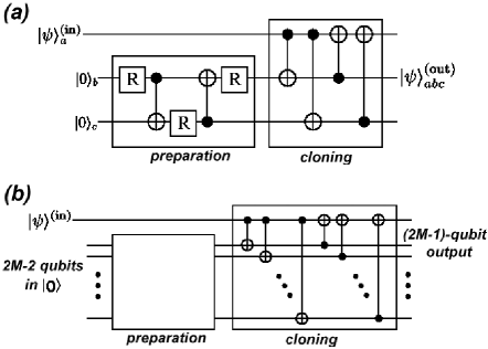
Figure 1: Quantum circuits for (a) $1\rightarrow 2$ UQCM, and (b) $1\rightarrow M$ UQCM. These circuits consist of two stages, namely the preparation and the copying stages. The preparation stage provides appropriate amplitudes for orthonormal bases according to Eqs. (2) or (4). The cloning stage permutes those amplitudes among all qubits, entangling them([13, 14]).

Eq. (2) was generalized by Gisin and Massar [3] to produce $M$ copies out of $N$ inputs. This transformation is described by

$$U_{N,M}|N\psi\rangle|0\rangle^{\otimes 2(M-N)} = \sum_{j=0}^{M-N}\alpha_{j}|(M-j)\psi,j\psi^{\perp}\rangle\otimes R_{j}(\psi),$$ (4)

$$\alpha_{j} = \sqrt{\frac{N+1}{M+1}}\sqrt{\frac{(M-N)!(M-j)!}{(M-N-j)!M!}},$$

$$R_{j}(\psi) = |(M-N-j)\psi^{*},j(\psi^{*})^{\perp}\rangle,$$

where $|N\psi\rangle$ is the input state consisting of $N$ qubits, all in the state $|\psi\rangle$. $|(M-j)\psi,j\psi^{\perp}\rangle$ is the symmetric and normalized state with $M-j$ qubits in the state $|\psi\rangle$ and $j$ qubits in the orthogonal state $|\psi^{\perp}\rangle$. $R_{j}(\psi)$ represent the internal state of the machine and $R_{j}(\psi)\perp R_{k}(\psi)$ holds for all $j\neq k$.

3 Generic Quantum Cloning Circuit

Bužek et al. constructed a quantum circuit for $1\rightarrow M$ UQCM which explicitly realizes Eq. (4) by generalizing the corresponding circuit for the $1\rightarrow 2$ case [16]. Figure 1(b) shows their circuit for $1\rightarrow M$ cloning machine. It is basically a natural extension of the $1\rightarrow 2$ circuit, consisting a preparation stage and a cloning (permutation) stage. Let us consider if it is possible to extend this $1\rightarrow M$ cloning circuit further to an $N\rightarrow M$ cloning circuit, by making up a circuit in Figure 2 in which the preparation stage is built up with both single and two qubit operations and the cloning stage is a sequence of CNOT or similar multi-qubit operation gates.

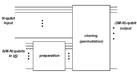
Figure 2: Quantum circuit for $N\rightarrow M$ UQCM? It turns out that this cloning circuit does work properly for any $M$ when $N=1$, $N=2$, and many other $N$ and $M$ as long as the condition (6) is fulfilled. If we are allowed to introduce additional auxiliary qubits inside the cloner, this circuit works for all combinations of $N$ and $M(>N)$.

Eq. (4) gives us a few hints on the possible construction of the quantum circuit for an $N\rightarrow M$ UQCM. First, $M-1$ qubits are necessary to represent the internal states of the machine. The total number of qubits needed to implement this transformation is $2M-N$.

Second, every basis of the form of $|(M-j)\psi,j\psi^{\perp}\rangle$ or $R_{j}(\psi)$ in Eq. (4) is a basis in the symmetrical subspace of the Hilbert space $\mathcal{H}^{\otimes M}$ or $\mathcal{H}^{\otimes(M-N)}$, where $\mathcal{H}$ is the space spanned by $|0\rangle$ and $|1\rangle$. Although the symmetrical subspace is a rather small subspace in the whole Hilbert space, almost all computational bases are involved in Eq. (4), especially when $N$ is small.

Therefore, almost $2^{2M-N}$ amplitudes need to be distributed to appropriate computational bases to perform the transformation (4), although the number of distinct amplitudes, $\alpha_{j}$, is only $M-N+1$. The fact that such a great number of amplitudes are necessary imposes a certain condition upon the values of $N$ and $M$ in order for an $N\rightarrow M$ cloning machine in Figure 2 to work properly.

Because the task of the cloning stage which consists of a sequence of CNOTs is to permute the amplitudes of all basis vectors which span the whole Hilbert space, all the amplitudes in Eq. (4), $\alpha_{j}$, must be provided by the preparation stage. Therefore, the preparation stage should be able to generate an entangled $2(M-N)$-qubit state with a set of any real amplitudes that may appear in Eq. (4) by adjusting the rotation angles of each single qubit gate.

For example, in the $1\rightarrow 2$ UQCM (Eq. (2) and Figure 1(a)), the amplitudes appearing in the output states are $\sqrt{\frac{2}{3}}$, $\sqrt{\frac{1}{6}}$, and $\sqrt{\frac{1}{6}}$. Thus, the preparation stage needs to provide these three coefficients and it turns out that, with the configuration of the cloning stage of Figure 1(a), the two-qubit state emerging from the preparation stage should be

$$|\psi\rangle^{\mathrm{prep}}=\sqrt{\frac{2}{3}}|00\rangle+\sqrt{\frac{1}{6}}|01\rangle+\sqrt{\frac{1}{6}}|11\rangle,$$ (5)

when the third qubit is used as the internal state of the machine. The rotation angles of the single qubit gates in this stage are determined accordingly.

However, this scheme only works when the number of distinct computational bases in Eq. (4) is smaller than the dimension of the Hilbert space that the preparation stage deals with. Otherwise, the preparation stage cannot generate enough amplitudes required by Eq. (4). This condition is written as

$$\sum_{k=0}^{M-N}{M\choose k}{M-N\choose k}\leq 2^{2(M-N)},$$ (6)

where the LHS represents the number of bases that appear in Eq. (4) and the RHS is the dimension of the Hilbert space where qubits in the preparation stage lie.

Eq. (6) is fulfilled for any $M$ when $N=1$, which is the case of Figure 1(b), and when $N=2$. Still, it becomes rather complicated when it comes to other combinations of $N$ and $M$. An example in which we can see the violation of Eq. (6) clearly is the case of $2N=M$, where the LHS of Eq. (6) for $N\gg 1$ can be estimated as

$$\sum_{k=0}^{N}{2N\choose k}{N\choose k}={3N\choose N}\simeq\sqrt{\frac{3}{4\pi}}\left(\frac{27}{4}\right)^{N}\frac{1}{\sqrt{N}}.$$ (7)

This always exceeds the corresponding RHS of Eq. (6), $2^{2N}$. Nevertheless, Eq. (6) is satisfied for $M$ which are sufficiently large compared with $N$, since its LHS is approximately $2^{2M-1}/\sqrt{\pi M}$, which is smaller than the RHS when $M>\pi^{-1}2^{4N-2}$.

Note that the condition (6) is not necessary if we are allowed to make use of more auxiliary qubits inside a cloning machine. Providing $2M-N$ qubits at most, instead of $2(M-N)$, enables the preparation stage to generate enough number of amplitudes for the cloning transformation. Then the cloning stage can complete the whole process by allocating those amplitudes to appropriate bases, leaving the auxiliary qubits disentangled, in state $|0\rangle$, from the legitimate $2M-N$ output qubits. Introducing these auxiliary qubits does not affect the estimation of the number of gates, which is discussed in the following.

Let us now count the number of elementary gates in the quantum cloning circuit, especially CNOT gates, as a CNOT gate takes a longer time to be performed than a single qubit gate [14].

The preparation stage should be designed so that it generates an arbitrary set of real amplitudes whose number is written by the LHS of Eq. (6). As far as the quantum cloning transformation Eq. (4) is concerned, the amplitudes should not necessarily be arbitrary as they are specifically described as in Eq. (4). However, in order to keep the full “controllability” on the output states, as in the case of $1\rightarrow 2$ UQCM, we assume that the preparation stage can generate arbitrary superpositions of $2^{d_{\mathrm{prep}}}$ bases with real amplitudes, where $d_{\mathrm{prep}}=2^{2(M-N)}$ is the dimension of the $2(M-N)$-qubit Hilbert space.

The transformation that the preparation stage performs can be written as $|00\cdots 0\rangle\rightarrow\sum_{k=0}^{d_{\mathrm{prep}}-1}c_{k}|k\rangle$, where $c_{k}$ are real numbers complying with the normalization condition $\sum_{k}c_{k}^{2}=1$. This is a unitary transformation which can be described by a $d_{\mathrm{prep}}\times d_{\mathrm{prep}}$ matrix, on the $d_{\mathrm{prep}}$-dimensional initial state vector $(1,0,\cdots,0)^{T}$, and its components are given by $u_{m1}=c_{m}$ and the rest of them are arbitrary for our purpose.

It is known that an outright circuit implementation of a $d\times d$ unitary matrix requires, in general, $O(d^{2}(\log d)^{2})$ elementary operations [17]. However, a more efficient circuit to create an arbitrary quantum superposition starting from $|00\cdots 0\rangle$ has been proposed in [18] and its complexity is given by $O(d(\log d)^{2})$. Thus we simply take $O(d_{\mathrm{prep}}(\log d_{\mathrm{prep}})^{2})$ as the number of CNOTs in the preparation stage of a UQCM in the following calculations.

The cloning stage is also generically hard to construct. The only exception we know of is the case of $1\rightarrow M$ UQCM, which can be realized by the circuit in Figure 1(b). In a more generic $N\rightarrow M$ case, we can build up a circuit as follows. As mentioned above, the cloning stage only permutes all bases with non-zero amplitudes among all computational bases of $\mathcal{H}^{\otimes(2M-N)}$. Thus, we can estimate the number of gates with only the knowledge of number of bases involved, even if we have no information on the actual permutation, i.e. which basis goes to which.

Table 1: The permutation of computational bases performed in the cloning stage of the $1\rightarrow 2$ quantum cloning circuit. The choice of bases on the left hand side follows Eq. (5).

Initial basis	$\rightarrow$	Final basis
$|000\rangle$	$\rightarrow$	$|000\rangle$
$|001\rangle$	$\rightarrow$	$|101\rangle$
$|011\rangle$	$\rightarrow$	$|011\rangle$
$|100\rangle$	$\rightarrow$	$|111\rangle$
$|101\rangle$	$\rightarrow$	$|010\rangle$
$|111\rangle$	$\rightarrow$	$|100\rangle$

Let us take the $1\rightarrow 2$ quantum cloning circuit as an example to simplify our description of its construction, although its efficient circuit is already given in Figure 1. Table 1 shows all the necessary permutations of bases to complete the transformation from Eq. (5) to Eq. (2). This permutation can be implemented as a circuit by carrying out each transformation one by one. Since $|010\rangle$ is not used in the preparation state, $|101\rangle\rightarrow|010\rangle$ should be performed first, otherwise any other destination state may be used as a preparation state later and thus the preceding transformation comes to naught. A basis which is exempted from being used in the preparation, such as $|010\rangle$ in this case, always exists in a more general $N\rightarrow M$ case as the equality in condition (6) never holds for $N,M\in\mathrm{I\!\!\!\;N}$. Hence, the appropriate order of transformation is $|101\rangle\rightarrow|010\rangle,|001\rangle\rightarrow|101\rangle,|111\rangle\rightarrow|001\rangle,|100\rangle\rightarrow|111\rangle,|001\rangle\rightarrow|100\rangle$, where $|001\rangle$ is used as a buffer in the last three operations, as it is not used in the final state, to swap $|100\rangle$ and $|111\rangle$.

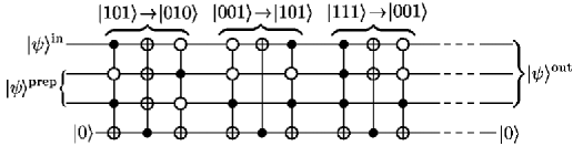
Figure 3: The quantum circuit for the permutation of bases. This figure depicts a circuit for the cloning stage of $1\rightarrow 2$ UQCM. An additional ancilla qubit is introduced as a flag to flip bits. Although there exists a much more efficient circuit for the same process, which is shown in Figure 1(a), this circuit can be applied to the UQCM with more input qubits, as in Figure 5.

Figure 3 shows a general way to permute bases. In this figure, an unfilled circle, $\circ$, denotes a control bit in-between two NOT gates. Unlike a filled circle $\bullet$, $\circ$ activates connected operations when the bit value at $\circ$ is $0$.

Here, an ancilla qubit is introduced in order to flip the incoming binary numbers according to the permutation required for a UQCM, as shown in Table 1. Finding a circuit for the basis permutation without ancillas is generally very hard, hence we make use of it here for convenience. The ancilla is prepared by the UQCM in a state $|0\rangle$ and it ends up in the same state $|0\rangle$ after the whole process. As the ancilla qubit is necessarily disentangled by the end of the process, we do not have to take it as a part of the output state.

In the earlier paragraph of this section, we have identified the generic features required of a copying circuit. For concreteness, it is important to show a specific example and in the following we do this for a $2\rightarrow 4$ cloner. Our circuit is not unique and other examples of course can be found.

The transformation of the state $|00\rangle$ by the $2\rightarrow 4$ quantum cloning can be written from Eq. (4) as

$$|00\rangle|0000\rangle \rightarrow \sqrt{\frac{3}{5}}|0000\rangle|11\rangle$$ (8)

$$+\sqrt{\frac{3}{80}}(|0001\rangle+|0010\rangle+|0100\rangle+|1000\rangle)(|01\rangle+|10\rangle),$$

$$+\sqrt{\frac{1}{60}}(\overbrace{|0011\rangle+\cdots+|1100\rangle}^{6\>\mathrm{bases}})|00\rangle,$$

and the transformation for $|11\rangle|0000\rangle$ can be obtained by flipping every bit in Eq. (8).

As mentioned earlier in this section, we need four qubits for the preparation stage in addition to two input qubits, thus, six qubits in total. The preparation stage generates all amplitudes for the 15 bases appearing in Eq. (8). The output from the preparation stage is, for example,

$$|0000\rangle\rightarrow|\psi\rangle^{\mathrm{prep}} = \sqrt{\frac{3}{5}}|0000\rangle+\sqrt{\frac{3}{80}}(\overbrace{|0001\rangle+\cdots+|1000\rangle}^{8\>\mathrm{bases}})$$ (9)

$$+\sqrt{\frac{1}{60}}(\overbrace{|1001\rangle+\cdots+|1110\rangle}^{6\>\mathrm{bases}}).$$

The quantum circuit to carry out this transformation is given in [18] and is also depicted in Figure 4. The boxes represent a single qubit operation $U_{\theta}$ of the form

$$U_{\theta}=\left(\begin{array}[]{cc}\cos\theta&\sin\theta\\ \sin\theta&-\cos\theta\end{array}\right),$$ (10)

and all $\theta$ in Figure 4 are given by

$$\theta_{1}=\tan^{-1}\sqrt{\frac{11}{69}},\>\>\>\theta_{20}=\tan^{-1}{\sqrt{\frac{4}{19}}},\>\>\>\theta_{21}=\tan^{-1}{\sqrt{\frac{4}{7}}},$$

$$\theta_{30}=\tan^{-1}{\sqrt{\frac{2}{17}}},\>\>\theta_{31}=\frac{\pi}{4},\>\>\theta_{32}=\tan^{-1}{\sqrt{\frac{8}{13}}},\>\>\theta_{33}=\tan^{-1}{\frac{1}{\sqrt{2}}},$$

$$\theta_{40}=\tan^{-1}{\frac{1}{4}},\theta_{41}=\theta_{42}=\theta_{43}=\theta_{45}=\theta_{46}=\frac{\pi}{4},\theta_{44}=\tan^{-1}{\frac{2}{3}},\theta_{47}=0,$$ (11)

One possible permutation of bases that achieves the transformation (8) from $|\psi\rangle^{\mathrm{prep}}$ in Eq. (9) is shown in Table 2. This can be implemented by the quantum circuit in Figure 5. With the quantum circuits of Figures 4 and 5, the quantum cloning transformation (8) is carried out faithfully and the upper three qubits in Figure 5 will be the clones, while the next two qubits are the state of the cloner and the lowest disentangled qubit is an ancilla which can be discarded.

Figure 4: The preparation stage for $2\rightarrow 4$ quantum cloning circuit. Angles $\theta$ in boxes are given by Eqs. (11).

Table 2: The permutations of bases to complete the transformation Eq. (8) when the circuit of the preparation is given by Figure 4. Many of them are omitted in this table since they are almost obvious by comparing Eq. (8) and Eq. (9).

Initial basis	$\rightarrow$	Final basis	Initial basis	$\rightarrow$	Final basis
$|000000\rangle$	$\rightarrow$	$|000011\rangle$	$|110000\rangle$	$\rightarrow$	$|111100\rangle$
$|000001\rangle$	$\rightarrow$	$|000101\rangle$	$|110001\rangle$	$\rightarrow$	$|111001\rangle$
$|000010\rangle$	$\rightarrow$	$|000110\rangle$	$|110010\rangle$	$\rightarrow$	$|111010\rangle$
$|000011\rangle$	$\rightarrow$	$|001001\rangle$	$|110011\rangle$	$\rightarrow$	$|110101\rangle$
$\vdots$	$\vdots$	$\vdots$	$\vdots$	$\vdots$	$\vdots$
$|001101\rangle$	$\rightarrow$	$|101000\rangle$	$|111101\rangle$	$\rightarrow$	$|101011\rangle$
$|001110\rangle$	$\rightarrow$	$|110000\rangle$	$|111110\rangle$	$\rightarrow$	$|110011\rangle$

Figure 5: The cloning stage for the $2\rightarrow 4$ quantum cloning circuit. Only four permutations $|000011\rangle\rightarrow|001001\rangle$, $|000100\rangle\rightarrow|001010\rangle$, $|000000\rangle\rightarrow|000011\rangle$, and $|110011\rangle\rightarrow|110101\rangle$ are shown. Each of these permutations consists of three multi-qubit control operations. This figure represents only one possible example because the order of permutation is not unique.

We can now estimate the number of CNOTs in the whole cloning circuit. In [19], the number of basic operations, i.e. single qubit operations and CNOTs, to simulate a multi-qubit controlled operation has been given as $O(n^{2})$ for a controlled-$U$ gate with $n-1$ control qubits and one auxiliary qubit. Therefore, the upper bound for the number of CNOTs in the cloning stage is the order of the number of bases involved, which is approximately twice of the number of amplitudes produced in the preparation stage, multiplied by the square of the number of qubits. As the number of the bases is given by the RHS of Eq. (6), $O(2^{2M}M^{-{\frac{1}{2}}})$, and there are $O(2^{2(M-N)}(M-N)^{2})$ CNOTs in the preparation stage, a quantum cloning circuit of the type of Figure 2 contains $O(2^{2M}(M-N)^{2}(2^{-2N}+M^{-{\frac{1}{2}}}))$ CNOTs at most in total.

This circuit looks rather inefficient especially because of the preparation stage. The inefficiency comes partly from our requirement that the preparation stage should be able to generate arbitrary superpositions. If both $N$ and $M$ can be fixed and we do not have to control the parameters of each single qubit gate, the task of the preparation stage is much easier and the configuration of its circuit may well be much simpler and more efficient.

The cloning stage is also inefficient due to the complexity of the network for a general permutation. Despite the linear dependence on $M$ in the case of $1\rightarrow M$ UQCM, the number of CNOTs grows exponentially as $M$ increases when there are $N$ inputs, since each permutation is done one by one in our circuit. It might be possible to find a more efficient circuit, however, we have not succeeded.

4 Decoherence Time and Cloning Time

With the number of CNOT gates estimated in the previous section, we can now compare the cloning time $T$ with the decoherence time $\tau_{\mathrm{dec}}$. We focus on a quantum computing realization which makes use of cooled trapped ions [20]. In the following, we assume that spontaneous emissions are the only source of decoherence, and we only discuss the process without error correction codes. Going beyond these constraints will be discussed elsewhere.

The Hamiltonian operator for a two-level ion of mass $m$, interacting with a phonon as a result of the centre-of-mass (c.m.) motion with frequency $\nu$, is then given by [20, 14],

$$H=\frac{\eta}{\sqrt{2M-N}}\frac{\Omega_{1}}{2}[|1\rangle\langle 0|a+|0\rangle\langle 1|a^{{\dagger}}],$$ (12)

where $\eta=(2\pi/\lambda)\sqrt{\hbar/2m\nu}$ is the Lamb-Dicke parameter, $\Omega_{1}$ is the Rabi frequency of the $0\leftrightarrow 1$ transition with 0 and 1 denoting the ground and the excited states of the ion. The $a$ and $a^{{\dagger}}$ are the annihilation and creation operators of the phonon. As in the original proposal [20], we assume that qubits are encoded in the internal state of ions and the phonons are used as the information bus. The denominator $\sqrt{2M-N}$ is a consequence of the fact that an $N\rightarrow M$ UQCM network needs $2M-N$ qubits (ions).

The elementary time step for a CNOT gate with this system can be written as

$$\tau_{\mathrm{el}}\simeq\frac{4\pi\sqrt{2M-N}}{\eta\Omega_{1}}.$$ (13)

The total processing time for cloning is

$$T\simeq\frac{4\pi\sqrt{2M-N}}{\eta\Omega_{1}}\epsilon 2^{2M+2}(M-N)^{2}\left(\frac{1}{2^{2N}}+\frac{1}{\sqrt{\pi M}}\right),$$ (14)

where $\epsilon$ is a some proportion factor. Here, we use the number of CNOTs in the preparation stage, because it is usually dominant over that of CNOTs in the cloning stage, as mentioned above. Also, we assume that all the CNOTs are performed sequentially one by one, despite the possibility of building up a circuit which performs several operations in parallel. Thus, the discussion below gives only a naive upper bound for the number of cloneable qubits. To minimize $T$, we wish to increase the value for $\Omega_{1}$, which is related to the decay rate of the excited state by [14, 21]

$$\frac{\Omega_{1}^{2}}{\Gamma_{1}}=\frac{6\pi c^{3}\epsilon_{0}}{\hbar\omega_{1}^{3}}E^{2},$$ (15)

where $E,c,\epsilon_{0}$, and $\omega_{1}$ are the electric field strength of the laser, the speed of light, the permittivity of vacuum, and the transition frequency between the states 0 and 1, respectively. Clearly, we would like to minimize the decoherence effects of $\Gamma_{1}$ by going to a metastable level, but then $\Omega_{1}$ is also small. We can increase the Rabi frequency $\Omega_{1}$ by increasing the electric field strength of the laser $E$, but it would then cause transitions to other higher levels which may be more rapidly decaying than state 1, and eventually spontaneous emissions which destroy the coherence of the system. Let $|2\rangle$ represent all other auxiliary levels which are coupled to the ground state $|0\rangle$.

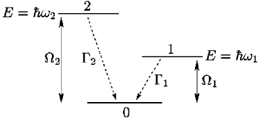
Figure 6: Three-level model of the ions used in a quantum cloner. The transition between 0 and 1 represents the qubit. An external laser drives this transition with Rabi frequency $\Omega_{1}$. The laser inevitably couples level 0 to other non-resonant levels such as level 2. The Rabi frequency of this transition is $\Omega_{2}$ and level 2 decays with a rate $\Gamma_{2}$.

As a stronger laser increases the population in the auxiliary level, it increases the rate of spontaneous emissions from level 2. Thus, we compute the probability of an emission from either level 1 and 2, and then minimize this probability to have an intensity-independent limit to the number of output qubits under the effect of spontaneous emission [21].

The probability of a spontaneous emission from the upper level of the qubit during the cloning process is

$$p_{1\rightarrow 0}={\frac{1}{2}}2\Gamma_{1}(2M-N)T.$$ (16)

The factor ${\frac{1}{2}}$ is present because we can assume that on average half of the qubits are in the upper level during the whole cloning period $T$. Because the auxiliary level is populated only when interacting with the laser, the probability of a spontaneous emission from level 2 is written as

$$p_{2\rightarrow 0}=\frac{\Omega_{2}^{2}}{8\Delta_{2}^{2}}2\Gamma_{2}T,$$ (17)

where $\Delta_{2}$ is the detuning between the frequency of the laser and that of the transition $0\leftrightarrow 1$. We now obtain the total probability of spontaneous emission

$$p_{\mathrm{total}} = p_{1\rightarrow 0}+p_{2\rightarrow 0}$$ (18)

$$= \frac{4\pi\epsilon\sqrt{(2M-N)^{3}\Gamma_{1}}}{\eta}2^{2M+2}(M-N)^{2}\left(\frac{1}{2^{2N}}+\frac{1}{\sqrt{\pi M}}\right)$$

$$\times\left[\frac{1}{x}+\frac{1}{2M-N}\left(\frac{\omega_{1}}{\omega_{2}}\right)^{3}\frac{\Gamma_{2}^{2}}{4\Delta_{2}^{2}\Gamma_{1}}x\right],$$

where $x=\Omega_{1}/\sqrt{\Gamma_{1}}$ and we used

$$\frac{\Omega_{1}^{2}}{\Gamma_{1}}=\left(\frac{\omega_{2}}{\omega_{1}}\right)^{3}\frac{\Omega_{2}^{2}}{\Gamma_{2}},$$

which is derived from Eq. (15). The minimum value of $p_{\mathrm{total}}$ with respect to $x$ is

$$p_{\mathrm{min}}=\frac{\pi\epsilon}{\eta}\left(\frac{\omega_{1}}{\omega_{2}}\right)^{\frac{3}{2}}\frac{\Gamma_{2}}{\Delta_{2}}2^{2M+4}(2M-N)(M-N)^{2}\left(\frac{1}{2^{2N}}+\frac{1}{\sqrt{\pi M}}\right).$$ (19)

In order for the cloning process to be successful, $p_{\mathrm{min}}$ should be very small compared with unity. This requirement gives the upper bound on $M$ for a given $N$ in the expression of

$$2^{2M_{\mathrm{max}}}(2M_{\mathrm{max}}-N)(M_{\mathrm{max}}-N)^{2}\left(\frac{1}{2^{2N}}+\frac{1}{\sqrt{\pi M_{\mathrm{max}}}}\right)$$

$$\simeq\frac{\eta}{2^{4}\pi\epsilon}\left(\frac{\omega_{2}}{\omega_{1}}\right)^{\frac{3}{2}}\frac{\Delta_{2}}{\Gamma_{2}}.$$ (20)

Table 3 shows the results of the actual calculations of the RHS of Eq. (4) for those ions often utilized in trap experiments along with their numerical data. Assuming $\epsilon=100$ [22], $\eta=0.01$ and $\Delta_{2}=10^{13}\>\,[s^{-1}]$, we find that Eq. (4) has no solutions for $M\geq 2$ as the LHS of Eq. (4) is equal to 31.2 when $N=1$ and $M=2$. However, if we consider only the $1\rightarrow 2$ cloning network, where the number of CNOTs is six according to Figure 1(a), the probability of spontaneous emission during the whole process becomes rather small. For example, $p_{\mathrm{min}}=0.062$ for $\mathrm{Ca^{+}}$ and $p_{\mathrm{min}}=0.017$ for $\mathrm{Ba^{+}}$, therefore the cloning may be successful.

Table 3: Atomic data of several possible systems for a quantum cloning machine and the RHS of Eq. (4), which should be smaller than the LHS. We can see that Eq. (4) has no solutions for $N>1$ and $M>2$, as its LHS, which is equal to 31.15 when $N=1$ and $M=2$, is always larger than the RHS shown in this table. Atomic data are taken from [21].

Ion	$\mathrm{Ca^{+}}$	$\mathrm{Hg^{+}}$	$\mathrm{Ba^{+}}$
level 0	$4s^{\,2}\!S_{1/2}$	$5d^{\,10}6s^{2\>\,2}\!S_{1/2}$	$6s^{\,2}\!S_{1/2}$
level 1	$3d^{\,2}\!D_{5/2}$	$5d^{\,9}6s^{2\>\,2}\!D_{5/2}$	$5d^{\,2}\!D_{5/2}$
level 2	$4s^{\,2}\!P_{3/2}$	$5d^{\,10}6p^{2\>\,2}\!P_{1/2}$	$6s^{\,2}\!P_{3/2}$
$\omega_{1}\>[s^{-1}]$	$2.62\times 10^{15}$	$6.7\times 10^{15}$	$1.07\times 10^{15}$
$\omega_{2}\>[s^{-1}]$	$4.76\times 10^{15}$	$11.4\times 10^{15}$	$4.14\times 10^{15}$
$\Gamma_{2}\>[s^{-1}]$	$67.5\times 10^{6}$	$5.26\times 10^{8}$	$58.8\times 10^{6}$
RHS of Eq. (4) $(\eta=0.01)$	$0.72$	$0.084$	$2.58$

Overall, we see that even for a small number of outputs copied from one input the decoherence due to spontaneous emissions plays a critical role. If we make an optimistic assumption for $\eta$, as $\eta=1.0$, $1\rightarrow 2$ cloning with $\mathrm{Ca^{+}}$, $1\rightarrow 2$ and $2\rightarrow 3$ with $\mathrm{Ba^{+}}$ would become possible.

If we are allowed to have one more auxiliary qubit, the number of basic operations to simulate a $(n-2)$-controlled operation can be reduced from $O(n^{2})$ to $O(n)$ [19]. Replacing the corresponding factors in the above calculations shows that, with $\eta=1.0$, $1\rightarrow 2$, $1\rightarrow 3$, and $2\rightarrow 3$ cloning may be possible with $\mathrm{Ba^{+}}$ as well as $1\rightarrow 2$ and $1\rightarrow 3$ cloning with $\mathrm{Ca^{+}}$.

5 Summary

We have first investigated a possible method to construct an $N\rightarrow M$ quantum cloning circuit in order to estimate the number of CNOT gates in it. We have estimated the number of CNOTs as $O(2^{2M}(M-N)^{2}(2^{-2N}+M^{-{\frac{1}{2}}}))$, with $N$ and $M$ the numbers of input and output qubits, respectively. Therefore, the number of gates in the quantum cloning circuit of the type of Figure 1(b) or Figure 2 is always exponential with respect to the number of output qubits.

With the circuit complexity we obtained, it has been shown that the quantum cloning may be implemented by using the system of trapped ions for only a few combinations of small $N$ and $M$, when the system is not immune to decoherence due to spontaneous emissions, provided sophisticated quantum error correction codes are not used. As spontaneous emissions are the only source of decoherence we have considered here, the number of possible combinations of $N$ and $M$ might be lowered further by taking into account of other effects, such as phonon decoherence [23], the random phase fluctuations of the lasers, the heating of the ions’ vibrational motion [24, 11, 12, 13].

Nevertheless, unlike the case of factorization by Shor’s algorithm [14], producing many clones is not necessarily what we expect from the quantum cloning. Since even a few copied qubits may be useful in quantum information processing [10], our results should not be interpreted too pessimistically. Furthermore, the use of quantum error correction codes will surely ease the condition for upper bounds.

In [25], it was shown that a quantum information distributor, which is a modification of the quantum cloning circuit, can be used as a universal programmable quantum processor in a probabilistic regime. From this point of view, our estimation on the upper bound for the clones implies physical bounds on the realization of such a processor with trapped ions.

One interesting subject we have not considered here is the effect of decoherence on the quality of the clones. If we allow a processing time which is longer than the decoherence time, the fidelity between the input and output states will surely be lower than what we expect from Eq. (4). We might be able to find a tradeoff between the fidelity and the number of cloneable qubits to have “useful” clones in terms of practical quantum information processing.

References

- [1] W.K. Wootters and W.H. Zurek, Nature 299, 802 (1982).
- [2] V. Bužek and M. Hillery, Phys. Rev. A 54, 1844 (1996).
- [3] N. Gisin and S. Massar, Phys. Rev. Lett. 79, 2153 (1997).
- [4] N. Gisin, Phys. Lett. A 242, 1 (1998).
- [5] R.F. Werner, Phys. Rev. A 58, 1827 (1998).
- [6] V. Bužek and M. Hillery, Physics World 14, 25 (2001).
- [7] Y-F. Huang, W-L. Li, C-F. Li, Y-S. Zhang, Y-K. Jiang, and G-C. Guo, Phys. Rev. A 64, 012315 (2001); F. De Martini, V. Mussi, and F. Bovino, Opt. Comm. 179, 581 (2000).
- [8] A. Lamas-Linares, C. Simon, J.C. Howell, and D. Bouwmeester, Science 296, 712 (2002).
- [9] S. Fasel, N. Gisin, G. Ribordy, V. Scarani, and H. Zbinden, Phys. Rev. Lett. 89, 107901 (2002).
- [10] E.F. Galvão and L. Hardy, Phys. Rev. A 62, 022301 (2000).
- [11] M. Murao and P.L. Knight, Phys. Rev. A 58, 663 (1998).
- [12] D.F.V. James, Phys. Rev. Lett. 81, 317 (1998).
- [13] S. Schneider and G.J. Milburn, Phys. Rev. A 57, 3748 (1998).
- [14] M.B. Plenio and P.L. Knight, Phys. Rev. A 53, 2986 (1996), M.B. Plenio and P.L. Knight, Proc. R. Soc. Lond. A 453, 2017 (1997).
- [15] V. Bužek , S.L. Braunstein, M. Hillery, and D. Bruß, Phys. Rev. A 56, 3446 (1997).
- [16] V. Bužek , M. Hillery, and P.L. Knight, Fortschr. Phys. 46, 521 (1998).
- [17] M.A. Nielsen and I.L. Chuang, Quantum Computation and Quantum Information, Cambridge University Press, Cambridge (2000), p. 193.
- [18] G.L. Long and Y. Sun, Phys. Rev. A 64, 014303 (2001).
- [19] A. Barenco, C.H. Bennett, R. Cleve, D.P. DiVincenzo, N. Margolus, P. Shor, T. Sleator, J.A. Smolin, and H. Weinfurter, Phys. Rev. A 52, 3457 (1995).
- [20] J.I. Cirac and P. Zoller, Phys. Rev. Lett. 74, 4091 (1995).
- [21] D. Bouwmeester, A. Ekert, and A. Zeilinger (Eds,) The Physics of Quantum Information, Springer-Verlag, Berlin (2000), pp. 227–232.
- [22] This is a rough estimation based on Corollary 7.4 in [19].
- [23] A. Garg, Phys. Rev. Lett. 77, 964 (1996).
- [24] R.J. Hughes, D.F.V. James, E.H. Knill, R. Laflamme, and A.G. Petschek, Phys. Rev. Lett. 77, 3240 (1996).
- [25] M. Hillery, V. Bužek , and M. Ziman, Phys. Rev. A 65, 022301 (2002).