Remote state preparation and teleportation in phase space

Abstract

Continuous variable remote state preparation and teleportation are analyzed using Wigner functions in phase space. We suggest a remote squeezed state preparation scheme between two parties sharing an entangled twin beam, where homodyne detection on one beam is used as a conditional source of squeezing for the other beam. The scheme works also with noisy measurements, and provide squeezing if the homodyne quantum efficiency is larger than $50\%$. Phase space approach is shown to provide a convenient framework to describe teleportation as a generalized conditional measurement, and to evaluate relevant degrading effects, such the finite amount of entanglement, the losses along the line, and the nonunit quantum efficiency at the sender location.

1 Introduction

Let us consider an entangled state described by a density matrix $R$ on a bipartite Hilbert space ${\cal H}_{1}\otimes{\cal H}_{2}$. A measurement performed on one subsystem reduces the other one according to the projection postulate. Each possible outcome, say $x$, occurs with probability $p_{x}$, and corresponds to a different conditional state $\varrho_{x}$

$$p_{x}=\hbox{Tr}_{12}\left[R\>\Pi_{x}\otimes I_{2}\right]\>,\qquad\varrho_{x}=\frac{1}{p_{x}}\hbox{Tr}_{1}\left[R\>\Pi_{x}\otimes I_{2}\right]\>.$$ (1)

$\Pi_{x}$ is the probability measure (POVM) of the measurement (acting on the Hilbert space of the first subsystem) and $I_{2}$ the identity operator on the second Hilbert space. $\hbox{Tr}_{12}\left[...\right]$ denotes full trace, whereas $\hbox{Tr}_{j}\left[...\right]$, $j=1,2$ denotes partial traces.

Eq. (1) shows that entanglement and conditional measurements can be powerful resources to realize (probabilistically) nonlinear dynamics that otherwise would not have been achievable through Hamiltonian evolution in realistic media. Since entanglement may be shared between two distant users (the sender performing the measurement, and the receiver observing the conditional output), the inherent nonlocality of entangled states permits the remote preparation of the conditional states $\varrho_{x}$, a protocol that may be used to exchange quantum information between the two parties sending only classical bits [1]. A different kind of remote state preparation is teleportation [2], where the measurement depends on an unknown reference state which may be recovered at the receiver location independently on the outcome of the measurement.

In this paper, we focus our attention on continuous variable (CV) remote state preparation . In particular, we analyze in detail an optical scheme for remote preparation of squeezed states by realistic (noisy) conditional homodyining. Our analysis is based on a phase-space approach, and this is motivated by the following reasons: i) entanglement in optical CV quantum information processing is provided by the so-called twin-beam (TWB) state of two field modes $|\lambda\rangle\rangle=\sqrt{1-\lambda^{2}}\sum_{p}\lambda^{p}\>|p\rangle|p\rangle$, $0<\lambda<1$; the corresponding Wigner function is Gaussian; ii) trace operation corresponds to overlap integral [5], and the Wigner function of (realistic) homodyne POVM is also a Gaussian. By Wigner calculus we will be able to derive simple analytical formulas for conditional outputs, also in the case of noisy measurement at the sender location. In addition, we will show that phase-space approach is a convenient framework to describe CV teleportation as a conditional measurement , and to evaluate relevant degrading effects, such the finite amount of entanglement, the losses along the transmission channel, and the nonunit quantum efficiency at the sender location.

2 Conditional measurement in phase space

TWB is the maximally entangled state (for a given, finite, value of energy) of two modes of radiation. It can be produced either by mixing two single-mode squeezed vacuum (with orthogonal squeezing phases) in a balanced beam splitter [3] or, from the vacuum, by spontaneous downconversion in a nondegenerate parametric optical amplifier (NOPA) [4]. The evolution operator of the NOPA reads as follows $U_{r}=\exp{\left[r\left(a^{\dagger}b^{\dagger}-ab\right)\right]}$ where the ”gain” $r$ is proportional to the interaction-time, the nonlinear susceptibility, and the pump intensity. We have $\lambda=\tanh r$, whereas the number of photons of TWB is given by $N=2\sinh^{2}r=2\lambda^{2}/(1-\lambda^{2})$. In view of the duality squeezing/entanglement via balanced beam-splitter [6] the parameter $r$ is sometimes referred to as the squeezing parameter of the twin-beam. Throughout the paper we will refer to mode $a$ as ”mode 1” and to mode $b$ as ”mode 2”. The Wigner function $W[\hbox{\footnotesize TWB}](x_{1},y_{1};x_{2},y_{2})$ of a TWB is Gaussian, and is given by (we omit the argument)

$$W[\hbox{\footnotesize TWB}]=\left(2\pi\sigma_{+}^{2}\>2\pi\sigma_{-}^{2}\right)^{-1}\>\exp\left[-\frac{(x_{1}+x_{2})^{2}}{4\sigma_{+}^{2}}-\frac{(y_{1}+y_{2})^{2}}{4\sigma_{-}^{2}}-\frac{(x_{1}-x_{2})^{2}}{4\sigma_{-}^{2}}-\frac{(y_{1}-y_{2})^{2}}{4\sigma_{+}^{2}}\right]$$

where the variances are given by

$$\sigma^{2}_{+}=\frac{1}{4}\exp\{2r\}\qquad\sigma^{2}_{-}=\frac{1}{4}\exp\{-2r\}\;.$$ (2)

Specializing Eq. (1) for $R=|\lambda\rangle\rangle\langle\langle\lambda|$ we have

$$p_{x} = \langle\langle\lambda|\Pi_{x}\otimes I_{2}|\lambda\rangle\rangle=(1-\lambda^{2})\hbox{Tr}_{1}\left[\lambda^{a^{\dagger}a}\>\Pi_{x}\right]$$

$$\varrho_{x} = \frac{1}{p_{x}}\hbox{Tr}_{1}\left[|\lambda\rangle\rangle\langle\langle\lambda|\>\Pi_{x}\otimes I_{2}\right]\;,$$ (3)

where, in the expression of $p_{x}$, we have already performed the trace over the Hilbert space ${\cal H}_{2}$. In the following, the partial traces in Eq. (3) will be evaluated as overlap integrals in the phase space. The Wigner function of a generic operator $O$ is defined as the following complex Fourier transform

$$W[O](\alpha) = \int\frac{d^{2}\gamma}{\pi^{2}}e^{\alpha\bar{\gamma}-\bar{\alpha}\gamma}\>\hbox{Tr}\left[O\>D(\gamma)\right]\;,$$ (4)

where $\alpha$ is a complex number, and $D(\gamma)=e^{\gamma a^{\dagger}-\bar{\gamma}a}$ is the displacement operator. The inverse transformation reads as follows [7]

$$O=\int d^{2}\alpha\>W[O](\alpha)\>e^{-2|\alpha|^{2}}\>e^{2\alpha a^{\dagger}}\left(-\right)^{a^{\dagger}a}e^{2\bar{\alpha}a}\;$$ (5)

Using the Wigner function the trace between two operators can be written as

$$\hbox{Tr}\left[O_{1}\>O_{2}\right] = \pi\int d^{2}\beta\>W[O_{1}](\beta)\>W[O_{2}](\beta)\;.$$ (6)

2.1 Remote squeezed states preparation

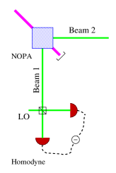
Let us consider the optical scheme depicted in Fig. 1. A TWB is produced by spontaneous downconversion in a NOPA, and then homodyne detection is performed on one of the two modes, say mode $1$. The POVM of the measurement, assuming perfect detection i.e. unit quantum efficiency, is given by

$$\Pi_{x}=|x\rangle\langle x|\qquad\qquad|x\rangle=\left(\frac{2}{\pi}\right)^{1/4}e^{-2x^{2}}\sum_{p}\frac{H_{p}(\sqrt{2}x)}{\sqrt{2^{p}p!}}|p\rangle\;,$$ (7)

$|x\rangle$’s being eigenstates of the quadrature operator $x=1/2(a+a^{\dagger})$. The Wigner function of the POVM $\Pi_{x}$ is a delta function

$$W[\Pi_{x}](x_{1})=\delta(x_{1}-x)\;,$$ (8)

whereas that of the term $\lambda^{a^{\dagger}a}$ in the first of Eqs. (3) is given by

$$(1-\lambda^{2})W[\lambda^{a^{\dagger}a}](x_{1},y_{1}) = (2\pi\sigma^{2})^{-1}\exp\left\{-\frac{x_{1}^{2}+y_{1}^{2}}{2\sigma^{2}}\right\}\>,$$ (9)

where the variance $\sigma$ depends on the number of photons of the TWB $\sigma^{2}=\frac{1}{4}(1+N)$. Using Eqs. (8) and (9) it is straightforward to evaluate the probability distribution

$$p_{x} = \!\!\int\!\!\!\!\int\!\!\!\!\int\!\!\!\!\int\!\!dx_{1}dy_{1}dx_{2}dy_{2}\>W[\hbox{\footnotesize TWB}](x_{1},y_{1};x_{2},y_{2})W[\Pi_{x}](x_{1})$$ (10)

$$= (1-\lambda^{2})\!\!\int\!\!\int\!\!\ dx_{1}dy_{1}\>W[\lambda^{a^{\dagger}a}](x_{1},y_{1})\>W[\Pi_{x}](x_{1})$$

$$= (2\pi\sigma^{2})^{-1/2}\exp\left\{-\frac{x^{2}}{2\sigma^{2}}\right\}\;,$$

and the Wigner function of the conditional output state

$$W[\varrho_{x}](x_{2},y_{2}) = \!\!\int\!\!\!\!\int\!\!dx_{1}dy_{1}\>W[\hbox{\footnotesize TWB}](x_{1},y_{1};x_{2},y_{2})W[\Pi_{x}](x_{1})$$ (11)

$$= (2\pi\Sigma_{1}^{2}\>2\pi\Sigma_{2}^{2})^{-1/2}\exp\left\{-\frac{(x_{2}-a_{x})^{2}}{2\Sigma_{1}^{2}}-\frac{y_{2}^{2}}{2\Sigma_{2}^{2}}\right\}\;.$$

The parameters in Eq. (11) are given by

$$a_{x}=\frac{\sqrt{N(N+2)}}{1+N}x\qquad\Sigma_{1}^{2}=\frac{1}{4}\frac{1}{1+N}\quad\Sigma_{2}^{2}=\frac{1}{4}(1+N)\;.$$ (12)

Eqs. (11) and (12) say that $\varrho_{x}$ is a squeezed-coherent minimum uncertainty state of the form $\varrho_{x}=D(a_{x})S(r_{x})|0\rangle$ i.e. a state squeezed in the direction of the measured quadrature $\overline{\Delta x^{2}}=1/4e^{-2r_{x}}$, with squeezing parameter given by $r_{x}=1/2\log(1+N)$. Notice that this result is valid for any quadrature $x_{\phi}=e^{ia^{\dagger}a\phi}xe^{-ia^{\dagger}a\phi}$, and therefore the present scheme, by tuning the phase of the local oscillator in the homodyne detection, is suitable for the remote preparation of squeezed states with any desired phase of squeezing. Of course, we have squeezing for $\varrho_{x}$ if and only if $N>0$ i.e. if and only if entanglement is present.

A question arises whether or not the remote preparation of squeezing is possible with realistic homodyne detection, i.e. with noisy measurement of the field quadrature. The POVM of a homodyne detector with quantum efficiency $\eta$ is a Gaussian convolution of the ideal POVM

$$\Pi_{x\eta}=\int\frac{dy}{\sqrt{2\pi\sigma_{\eta}^{2}}}\>\exp\{-\frac{(y-x)^{2}}{2\sigma_{\eta}^{2}}\}\>|y\rangle\langle y|\;,$$ (13)

with $\sigma_{\eta}^{2}=\frac{1}{4}(1-\eta)/\eta$ [8]. The corresponding Wigner function is given by

$$W[\Pi_{x\eta}](x_{1})=(2\pi\sigma_{\eta}^{2})^{-1/2}\exp\left\{-\frac{(x_{1}-x)^{2}}{2\sigma_{\eta}^{2}}\right\}\;.$$ (14)

Using (14) one evaluates the probability distribution and the Wigner function of the conditional output state, one has

$$p_{x\eta}=[2\pi(\sigma^{2}+\sigma_{\eta}^{2})]^{-1/2}\exp\left\{-\frac{x^{2}}{2(\sigma^{2}+\sigma_{\eta}^{2})}\right\}$$ (15)

$$W[\varrho_{x\eta}](x_{2},y_{2})=(2\pi\Sigma_{1\eta}^{2}\>2\pi\Sigma_{2\eta}^{2})^{-1/2}\exp\left\{-\frac{(x_{2}-a_{x\eta})^{2}}{2\Sigma_{1\eta}^{2}}-\frac{y_{2}^{2}}{2\Sigma_{2\eta}^{2}}\right\}\;,$$ (16)

where

$$a_{x\eta}=\frac{\eta\sqrt{N(N+2)}}{1+\eta N}x\qquad\Sigma_{1\eta}^{2}=\frac{1}{4}\frac{1+N(1-\eta)}{1+\eta N}\quad\Sigma_{2\eta}^{2}=\frac{1}{4}(1+N)\;.$$ (17)

As a matter of fact, the conditional output $\varrho_{x\eta}$ is no longer a minimum uncertainty state. However, for $\eta$ large enough, it still shows squeezing in the direction individuated by the measured quadrature i.e. $\overline{\Delta x^{2}}<1/4$. In order to obtain the explicit form of the conditional output state from the Wigner function $W[\varrho_{x\eta}](x_{2},y_{2})$ of Eq. (16) we use Eq. (5) arriving at

$$\varrho_{x\eta}=D(a_{x\eta})S(r_{x\eta})\nu_{th}S^{\dagger}(r_{x\eta})D^{\dagger}(a_{x\eta})\;,$$ (18)

where $\nu_{th}=(1+n_{th})^{-1}\sum_{p}[n_{th}/(1+n_{th})]^{p}\>|p\rangle\langle p|$ is a thermal state with average number of photons given by

$$n_{th} = \frac{1}{2}\left\{\sqrt{\frac{(1+N)[1+N(1-\eta)]}{1+\eta N}}-1\right\}\;,$$ (19)

and the squeezing parameter is given by

$$r_{x\eta} = \frac{1}{4}\log\frac{(1+N)(1+\eta N)}{1+N(1-\eta)}\;.$$ (21)

We have squeezing in $\varrho_{x\eta}$ if $\Sigma_{1\eta}^{2}<1/4$, and this happens for $\eta>50\%$ independently on the actual value $x$ of the homodyne outcome. The values of efficiency that can be currently realized in a quantum optical lab is far above the $50\%$ limit, and thus we conclude that conditional homodyning on TWB is a robust scheme for the remote preparation of squeezing.

2.2 Teleportation as a generalized conditional measurement

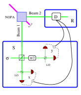
The scheme for optical CV teleportation is depicted in Fig. 2. One part of a TWB is mixed with a given reference state $\sigma$ in a balanced beam splitter, and two orthogonal quadratures $x=1/2(a+a^{\dagger})$, $y=i/2(a^{\dagger}-a)$ are measured on the outgoing beams by means of two homodyne detectors with local oscillators phase-shifted by $\pi/2$. The other part of the TWB is then displaced by an amount $-\alpha=-x-iy$ that depends on the outcome of the measurements, and the resulting state (averaged over the possible outcomes) is the teleported state.

Overall, the measurement performed on the TWB is a generalized double homodyne detection [9, 10] (equivalent to generalized heterodyne), which can be described by the POVM [10, 11]

$$\Pi_{\alpha}=D(\alpha)\sigma^{T}D^{\dagger}(\alpha)\;,$$ (22)

$...^{T}$ denoting transposition. Therefore, using Eq. (3), one has

$$p_{\alpha} = \langle\langle\lambda|\Pi_{\alpha}\otimes I_{2}|\lambda\rangle\rangle=(1-\lambda^{2})\hbox{Tr}_{1}\left[\lambda^{a^{\dagger}a}\>D(\alpha)\sigma^{T}D^{\dagger}(\alpha)\right]$$

$$\varrho_{\alpha} = \frac{1}{p_{\alpha}}D(-\alpha)\hbox{Tr}_{1}\left[|\lambda\rangle\rangle\langle\langle\lambda|\>D(\alpha)\sigma^{T}D^{\dagger}(\alpha)\otimes I_{2}\right]D^{\dagger}(-\alpha)\;,$$ (23)

while the teleported state is given by

$$\varrho=\int d^{2}\alpha\>p_{\alpha}\>\varrho_{\alpha}=\int d^{2}\alpha\>D(-\alpha)\hbox{Tr}_{1}\left[|\lambda\rangle\rangle\langle\langle\lambda|\>D(\alpha)\sigma^{T}D^{\dagger}(\alpha)\otimes I_{2}\right]D^{\dagger}(-\alpha)\;.$$ (24)

Using Wigner functions and taking into account that for any density matrix

$$W[\varrho^{T}](x,y)=W[\varrho](x,-y)$$ (25)

$$W[D(\alpha)\varrho D^{\dagger}(\alpha)](x,y)=W[\varrho](x-x_{\alpha},y-y_{\alpha})\;,$$ (26)

with $x_{\alpha}=\hbox{Re}[\alpha]$ and $y_{\alpha}=\hbox{Im}[\alpha]$, one has

$$W[\varrho](x_{2},y_{2})=$$

$$=\!\!\int\!\!\!\!\int\!\!dx_{1}dy_{1}\!\!\int\!\!\!\!\int\!\!dx_{\alpha}dy_{\alpha}\>W[\hbox{\footnotesize TWB}](x_{1},y_{1};x_{2}+x_{\alpha},y_{2}+y_{\alpha})\>W[\sigma](x_{1}-x_{\alpha},-y_{1}-y_{\alpha})$$

$$=\!\!\int\!\!\!\!\int\!\!dx_{1}dy_{1}\>W[\sigma](x_{1},y_{1})\int\!\!\!\!\int\!\!dx_{\alpha}dy_{\alpha}\>W[\hbox{\footnotesize TWB}](x_{1}+x_{\alpha},-y_{1}-y_{\alpha};x_{2}+x_{\alpha},y_{2}+y_{\alpha})$$

$$=\!\!\int\!\!\!\!\int\!\!\frac{dx_{1}dy_{1}}{\pi\kappa_{r}^{2}}\exp\left\{-\frac{(x_{1}-x_{2})^{2}+(y_{1}-y_{2})^{2}}{\kappa^{2}_{r}}\right\}\>W[\sigma](x_{1},y_{1})$$

$$=\!\!\int\!\!\!\!\int\!\!\frac{dx_{1}dy_{1}}{\pi\kappa_{r}^{2}}\exp\left\{-\frac{x_{1}^{2}+y_{1}^{2}}{\kappa^{2}_{r}}\right\}\>W[D(\alpha_{1})\sigma D^{\dagger}(\alpha_{1})](x_{2},y_{2})\;,$$ (27)

with $\alpha_{1}=x_{1}+iy_{1}$ and $\kappa_{r}^{2}=\exp\{-2r\}$. From Eqs. (27) and (5) one has that the teleported state is given by

$$\varrho=\int\frac{d^{2}\alpha}{\pi\kappa_{r}^{2}}\>\exp\{-\frac{|\alpha|^{2}}{\kappa_{r}^{2}}\}\>D(\alpha)\sigma D^{\dagger}(\alpha)\;,$$ (28)

which coincides with the input state only in the limit $r\longrightarrow\infty$ i.e. for infinite energy of the TWB. Eq. (28) shows that CV teleportation with finite amount of entanglement is equivalent to a thermalizing channel with $\kappa_{r}$ thermal photons: this results has been obtained also with other methods [12]. However, the present Wigner approach may be more convenient in order to include other degrading effects such the nonunit quantum efficiency at the sender location and the losses along the transmission channel.

Nonunit quantum efficiency at the homodyne detectors affects the POVM of the sender, which become a Gaussian convolution of the ideal POVM $\Pi_{\alpha}$

$$\Pi_{\alpha\eta}=\int\frac{d^{2}\beta}{\pi\Delta_{\eta}^{2}}\>\exp\{-\frac{|\alpha-\beta|^{2}}{\Delta_{\eta}^{2}}\}\>\Pi_{\beta}\;,$$ (29)

with $\Delta_{\eta}^{2}=(1-\eta)/\eta$ [8]. On the other hand, losses along the line degrade the entanglement of the TWB supporting the teleportation. The propagation of a TWB inside optical media can be modeled as the coupling of each part of the TWB with a non zero temperature reservoir. The dynamics can be described in terms of the two-mode Master equation

$$\frac{d\varrho_{t}}{dt}\equiv{\cal L}\varrho_{t}=\Gamma(1+M)L[a]\varrho_{t}+\Gamma(1+M)L[b]\varrho_{t}+\Gamma ML[a^{\dagger}]\varrho_{t}+\Gamma ML[b^{\dagger}]\varrho_{t}$$ (30)

where $\varrho_{t}\equiv\varrho(t)$, $\Gamma$ denotes the (equal) damping rate, $M$ the number of background thermal photons, and $L[O]$ is the Lindblad superoperator $L[O]\varrho_{t}=O\varrho_{t}O^{\dagger}-\frac{1}{2}O^{\dagger}O\varrho_{t}-\frac{1}{2}\varrho_{t}OO^{\dagger}\>.$ The terms proportional to $L[a]$ and $L[b]$ describe the losses, whereas the terms proportional to $L[a^{\dagger}]$ and $L[b^{\dagger}]$ describe a linear phase-insensitive amplification process. This can be due either to optical media dynamics or to thermal hopping; in both cases no phase information is carried. Of course, the dissipative dynamics of the two channels are independent on each other. The master equation (30) can be transformed into a Fokker-Planck equation for the two-mode Wigner function of the TWB Using the differential representation of the superoperators in Eq. (30) the corresponding Fokker-Planck equation reads as follows

$$\partial_{\tau}W_{\tau}=\left[\frac{1}{8}\left(\sum_{j=1}^{2}\partial^{2}_{x_{j}x_{j}}+\partial^{2}_{y_{j}y_{j}}\right)+\frac{\gamma}{2}\left(\sum_{j=1}^{2}\partial_{x_{j}}x_{j}+\partial_{y_{j}}y_{j}\right)\right]W_{\tau}\>,$$ (31)

where $\tau$ denotes the rescaled time $\tau=(\Gamma/\gamma)\>t$, and $\gamma=\frac{1}{2M+1}$ the drift term. The solution of Eq. (31) can be written as

$$W_{\tau} = \int dx^{\prime}_{1}\int dx^{\prime}_{2}\int dy^{\prime}_{1}\int dy^{\prime}_{2}\;\>W[\hbox{\footnotesize TWB}](x^{\prime}_{1},y^{\prime}_{1};x^{\prime}_{2},y^{\prime}_{2})\>\prod_{j=1}^{2}G_{\tau}(x_{j}|x^{\prime}_{j})G_{\tau}(y_{j}|y^{\prime}_{j})\>$$ (32)

where $W[\hbox{\footnotesize TWB}]$ is initial Wigner function of the TWB, and the Green functions $G_{\tau}(x_{j}|x^{\prime}_{j})$ are given by

$$G_{\tau}(x_{j}|x^{\prime}_{j})=\frac{1}{\sqrt{2\pi D^{2}}}\exp\left[-\frac{(x_{j}-x^{\prime}_{j}e^{-\frac{1}{2}\gamma\tau})^{2}}{2D^{2}}\right]\;,\quad D^{2}=\frac{1}{4\gamma}(1-e^{-\gamma\tau})\;.$$ (33)

The Wigner function $W_{\tau}$ can be obtained by the convolution (32), which can be easily evaluated since the initial Wigner function is Gaussian. The form of $W_{\tau}$ is the same of $W[\hbox{\footnotesize TWB}]$ with the variances changed to

$$\sigma_{+}^{2}\longrightarrow\left(e^{-\gamma\tau}\sigma_{+}^{2}+D^{2}\right)\qquad\sigma_{-}^{2}\longrightarrow\left(e^{-\gamma\tau}\sigma_{-}^{2}+D^{2}\right)\>.$$ (34)

Inserting the Wigner functions of the blurred POVM $\Pi_{\alpha\eta}$ and of the evolved TWB in Eqs. (23) and (24) we obtain the teleported state in the general case, which is still given by Eq. (28), with the parameter $\kappa_{r}$ now given by

$$\kappa_{r}^{2}\longrightarrow e^{-\Gamma t-2r}+(2M+1)(1-e^{-\Gamma t})+\Delta_{\eta}^{2}\;.$$ (35)

Eqs. (28) and (35) summarize all the degrading effects on the quality of the teleported state. In the special case of coherent state teleportation $\sigma=|z\rangle\langle z|$ (which corresponds to original optical CV teleportation experiments [3]) the fidelity $F=\langle z|\varrho|z\rangle$ can be evaluated straightforwardly as the overlap of the Wigner functions. Since $W[z](\alpha)=2/\pi\>e^{-2|\alpha-z|^{2}}$ is the Wigner function of a coherent state we have

$$F=\frac{1}{1+e^{-2r-\Gamma t}+(1-e^{-\Gamma t})(2M+1)+(1-\eta)/\eta}\>.$$

The condition on the fidelity, in order to assure that the scheme is a truly nonlocal protocol, is given by $F>1/2$ [3], i.e.

$$e^{-2r-\Gamma t}+(1-e^{-\Gamma t})(2M+1)+(1-\eta)/\eta<1\>.$$

Therefore, the bound on the quantum efficiency to demonstrate quantum teleportation is given by

$$\eta>\frac{1}{2-e^{-2r-\Gamma t}-(1-e^{-\Gamma t})(2M+1)}\>.$$

If the propagation induces low perturbation i.e. if $\Gamma\simeq 0$ and $M\simeq 0$ we have $\eta>(2-e^{-2r})^{-1}$, which ranges from $1/2$ to $1$, and represents the range of ”useful” values for the quantum efficiency. If $\Gamma$ and $M$ are not negligible then, for the same initial squeezing, we need a larger value of the quantum efficiency. Moreover, since quantum efficiency should be lower or equal to unit $\eta\leq 1$, we may derive a bound on the initial squeezing that allows to demonstrate quantum teleportation. This reads as follows $e^{-2r}\leq(2M+1)-2Me^{\Gamma t}$. Remarkably, if the number of thermal photons is zero, i.e. if the TWB is propagating in a zero temperature environment, then any value of the initial squeezing parameter make teleportation possible, of course if the quantum efficiency at the receiver location satisfies $\eta\geq(2-e^{-2r-\Gamma t}-1+e^{\Gamma t})^{-1}$.

3 Conclusions

A method for the remote preparation of squeezed states by conditional homodyninig on a TWB has been suggested. The scheme has been studied using Wigner function, which is the most convenient approach to describe effects of nonunit quantum efficiency at homodyne detectors. The method is shown to provide remote squeezing if the quantum efficiency is larger than $50\%$. Since downconversion correlates pair of modes at any frequencies $\omega_{1}$ and $\omega_{2}$ satisfying $\omega_{1}+\omega_{2}=\omega_{P}$, $\omega_{P}$ being the frequency of the pump beam, the present method can be used to generate squeezing at frequencies where no media for degenerate downconversion are available [13].

Phase-space approach has been also used to analyze CV teleportation as a conditional generalized double homodyning on a TWB. Also in this case the use of Wigner functions represents a powerful tool to evaluate the degrading effects of finite amount of entanglement, losses along the transmission channel, and nonunit quantum efficiency at sender location. A bound on the value of quantum efficiency needed to demonstrate quantum teleportation has been derived.

References

Figure 1: Schematic diagram of conditional homodyne for remote squeezed state preparation. A TWB is produced by spontaneous downconversion in a NOPA, and then homodyne detection is performed on one of the two modes, say mode $1$. Mode $2$ is squeezed if the homodyne quantum efficiency is larger than $50\%$.

Figure 2: Schematic diagram of teleportation scheme. In the sender area (S), one part of a TWB is mixed with a given reference state $\sigma$ (the state to be teleported) in a balanced beam splitter, and two orthogonal quadratures are measured on the outgoing beams by means of two homodyne detectors with local oscillators phase-shifted by $\pi/2$. After the measurement, in the receiver area (R), the other part of the TWB is displaced by an amount $-\alpha=-x-iy$ that depends on the outcome of the measurements itself. The overall state, averaged over the possible outcomes, is the teleported state.

References

• [1] A. K. Pati, Phys. Rev. A 63 (2001) 014302; Hoi-Kwong Lo, Phys. Rev. A 62, 012313 (2000).
• [2] C.H. Bennett et al., Phys. Rev. Lett. 70, 1895 (1993).
• [3] A. Furusawa et al., Science 282, 706 (1998).
• [4] O. Aytur, P. Kumar, Phys. Rev. Lett. 65, 1551 (1990).
• [5] K. Cahill, R. Glauber, Phys. Rev. 177, 1857 (1969); ibidem pag 1882.
• [6] M. G. A. Paris, Phys. Lett. A 225, 28 (1997).
• [7] G. M. D’Ariano and M. F. Sacchi, N. Cim. B 112, 881 (1997).
• [8] U. Leonhardt and H. Paul, Phys. Rev. A 48, 4598 (1993); G. M. D’Ariano et al., Phys. Lett. A 198, 286 (1995).
• [9] M. G. A. Paris, A. Chizhov, O. Steuernagel, Opt. Comm. 134, 117 (1997).
• [10] P. Busch , P. Lahti, Riv. Nuovo Cim. 18, 1 (1995).
• [11] M. G A Paris, in VII international conference on squeezed states and uncertainty relations, E-book http://www.wam.umd.edu/~ys/boston.html.
• [12] H. F. Hofmann et al., Phys. Rev. A 62, 062304 (2000); Masashi Ban et qal., preprint quant-ph/0202172.
• [13] A. Andreoni et al., Eur. Phys. Journ D 13, 415 (2001).
Refer to caption