Analytical study of four-wave mixing with large atomic coherence

Abstract

Four-wave mixing in resonant atomic vapors based on maximum coherence induced by Stark-chirped rapid adiabatic passage (SCRAP) is investigated theoretically. We show the advantages of a coupling scheme involving maximum coherence and demonstrate how a large atomic coherence between a ground and an highly excited state can be prepared by SCRAP. Full analytic solutions of the field propagation problem taking into account pump field depletion are derived. The solutions are obtained with the help of an Hamiltonian approach which in the adiabatic limit permits to reduce the full set of Maxwell-Bloch equations to simple canonical equations of Hamiltonian mechanics for the field variables. It is found that the conversion efficiency reached is largely enhanced if the phase mismatch induced by linear refraction is compensated. A detailed analysis of the phase matching conditions shows, however, that the phase mismatch contribution from the Kerr effect cannot be compensated simultaneously with linear refraction contribution. Therefore, the conversion efficiency in a coupling scheme involving maximum coherence prepared by SCRAP is high, but not equal to unity.

I Introduction

Nonlinear frequency conversion processes in atomic or molecular gases have attracted much attention since the early days of nonlinear optics. The interest is mainly motivated by the possibility to generate coherent radiation in the XUV and VUV frequency range, where there are no transparent nonlinear crystals. However, the conversion efficiencies are usually relatively poor due to small nonlinear susceptibility for the generation and difficulties to prepare proper phase matching conditions. Approaching atomic resonances enhances the nonlinearity, but at the same time absorption, linear refraction and unwanted nonlinear phase shifts increase rapidly.

Recently, a new technique has been put forward which substantially improves the nonlinear-optical properties of a medium. The technique, usually referred to as ”nonlinear optics with maximum coherence”, is based on the preparation of all atoms in the medium in the same coherent superposition of two states $\left|1\right\rangle$ and $\left|2\right\rangle$ with equal probability amplitudes jain96 . From the classical point of view, coherently prepared atoms represent an ensemble of dipoles all oscillating at the same frequency $\omega_{21}$, with the same phase and with maximum amplitude. If a radiation field of frequency $\omega_{3}$ is applied to the medium, it will beat against this strong local oscillator to produce the sum- or difference frequency $\omega_{21}\pm\omega_{3}$. In this case, the nonlinear susceptibility of the generation process is large (in fact, it is resonantly enhanced) and is of the same order as the linear susceptibility. Therefore, complete conversion occurs within an optical length smaller than the coherence length. Consequently, requirements for the phase matching are substantially alleviated and the influence of density-dependent detrimental effects is minimized.

In first proposals and experimental implementations jain96 ; mer99 , maximum coherence was established in a lambda-type coupling scheme with ground $\left|1\right\rangle$ and lower excited $\left|2\right\rangle$ states using stimulated Raman adiabatic passage (STIRAP) stirap . However, in a lambda-type coupling scheme involving one-photon transitions the generated radiation $\omega_{21}\pm\omega_{3}$ cannot reach far into the vacuum-ultraviolet spectral region mer99 . Multi-photon excitations may not be used in order to reach higher lying states, because laser-induced Stark shifts, which are intrinsic to multi-photon transitions, perturb the adiabatic population dynamics and prohibit the preparation of a maximum coherence mph-stirap .

In the present paper, we investigate the use the Stark Chirped Rapid Adiabatic Passage (SCRAP) technique scrap ; h-scrap ; pop to prepare maximum coherence. In SCRAP, a pump laser couples a thermally populated state (most likely the ground state) to an excited state and a second, strong radiation pulse to induce a dynamic Stark shift. This Stark shift serves to sweep the atomic transition frequency through resonance with the pump laser frequency, mediating thereby an adiabatic passage of population between two states. Provided the dynamic Stark shifts, induced by the second laser are larger than the shifts, induced by the pump field, any multi-photon transition may be used for the pump transition. For a two-photon pump transition, it is therefore possible to create coherence between a highly excited state and the ground state. If ultraviolet radiation is used for the pump laser, coherence between states with energies up to 10 eV may be efficiently created, permitting the generation of VUV radiation well below 150 nm.

The potential of the nonlinear optics with maximum coherence has been demonstrated for the regime of undepleted coherence and hence for an undepleted pump field jain96 . We consider here a process of difference-frequency mixing involving a two-photon transition $\left|1\right\rangle-\left|2\right\rangle$ resonantly excited by a strong pump field with frequency $\omega_{1}$ and a dipole-allowed transition $\left|2\right\rangle-\left|3\right\rangle$ excited off-resonance by an ”idler” field with frequency $\omega_{2}$ (Fig. 1). In this case, energy for the generated field is taken only from the pump field, which at the same time participates in the preparation of the coherence. Therefore, it will unavoidably be depleted if considerable conversion efficiency is expected. It is the aim of the present work to clarify, how the conversion proceeds when the pump field is depleted, what fraction of the total energy of the pump field may be transferred to the generated (and idler) field, and which parameters are needed in the specific case of coherence preparation by SCRAP. To this end, we solve the nonlinear propagation problem taking into account the pump field depletion. The solution of such a nonlinear problem is particularly challenging for pulses and is in general possible only numerically. In order to obtain analytical solutions we apply the so-called Hamiltonian approach mel79 ; kryz ; kors02 which allows for a solution in a wide range of physically relevant situations. An essence of this formalism is to reduce a set of Maxwell propagation equation to canonical Hamilton equations of classical mechanics, which admit several integrals of motion. Additionally, this approach allows to analyze phase matching conditions taking into account intensity-dependent (Kerr effect) contributions, which are not present in the simple treatment of undepleted coherence. This approach is especially useful under adiabatic conditions, i.e. when the atoms are excited by the laser pulses in such a way that they remain in the same instantaneous eigenstate of the interaction Hamiltonian during the entire process. This is the case in the atomic superposition prepared by SCRAP, as it is discussed here.

Obviously the large atomic coherence should be maintained for the duration of the conversion process. Since the coherent superposition includes a highly excited state, this requirement restricts the conversion to a regime with laser pulses of duration shorter than the natural lifetimes in the system. This is however not in contradiction with the adiabaticity of SCRAP. The adiabatic approximation requires a slow rate of evolution as compared to the frequency separation of the adiabatic eigenstates. This results usually in a requirement for the product of the pulse duration and the Rabi frequency of the radiation field to be much larger than unity. Thus, for sufficiently intense fields, the process can be adiabatic even for short pulses. In the present paper, we consider the frequency conversion of short pulses and disregard spontaneous relaxation processes.

The paper is organized as follows. In Sec.II we discuss general features and advantages of nonlinear frequency conversion processes with respect to atomic coherence. The coherence is assumed to be undepleted. In Sec. III the preparation of large atomic coherence by SCRAP is described. Sec. IV and the Appendix outline the Hamiltonian approach in nonlinear optics. Making use of this formalism we derive analytic solutions for frequency conversion processes involving maximum coherence in Secs.V, VI. Section V is devoted to solutions at small propagation distances in which the pump field is not depleted. Conclusions of Sec. II are confirmed and specific phase matching conditions for the SCRAP method are derived. In Sec. VI full analytical solutions are obtained taking into account depletion of the driving field. In Sec. VII we discuss the conditions for phase matching with respect to the compensation of phase mismatch, induced by linear refraction and the Kerr effect simultaneously. Finally, in Sec. VIII, we consider the spatio-temporal dynamics of the generated radiation pulse as well as the evolution of the total conversion efficiency. Conclusions are presented in Sec. IX.

II Frequency conversion with undepleted atomic coherence

The (pulsed) e.m. field propagating in an ensemble of three-level atoms (Fig. 1) is assumed to consist of three components with carrier frequencies $\omega_{1},\omega_{2}$ and $\omega_{3}=2\omega_{1}-\omega_{2}$:

$$E(z,t)=\sum_{j}\left(\mathcal{E}_{j}(z,t)\exp(-i(\omega_{j}t-\mathbf{k}_{j}\mathbf{r}))+c.c.\right).$$ (1)

Here $\left|\mathbf{k}_{j}\right|=n_{j}\omega_{j}/c$ with the refractive index $n_{j}$ at frequency $\omega_{j}$ describing refraction due to levels outside the three-level system in Fig. 1. The radiation pulses are supposed to be shorter than the relaxation times in the atomic system. The waves $\mathbf{k}_{2}$ and $\mathbf{k}_{3}$ propagate at small angles with respect to the vector $\mathbf{k}_{1}$ (the $z$ axis).

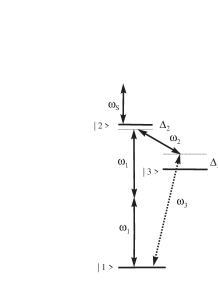
Figure 1: Resonant four-wave mixing with maximum coherence between $|1\rangle$ and $|2\rangle$ adiabatically prepared by a strong drive $\omega_{1}$ field and a ”Stark-shifting” far-off-resonance $\omega_{s}$ field.

In the approximation of slowly varying amplitudes and phases Maxwell’s propagation equations read in a moving frame

$$\frac{\partial\mathcal{E}_{j}}{\partial z}=i2\pi\frac{\omega_{j}}{c}\mathcal{P}_{j},$$ (2)

where $\mathcal{E}_{j}$ and $\mathcal{P}_{j}$ ($j=1,2,3$) are functions of the coordinate $z$ and the retarded time $\tau=t-z/c$.

$\mathcal{P}_{j}$ are the components of the medium polarization:

$$P=\sum_{j}\Bigl{(}\mathcal{P}_{j}\exp(-i(\omega_{j}t-\mathbf{k}_{j}\mathbf{r}))+c.c.\Bigr{)}.$$

The pulse at frequency $\omega_{s}$ (”ac Stark-shifting pulse”) propagates along the $z$ axis and is far detuned from any atomic state. Therefore, we assume that its intensity does not change along the propagation path. In reality, the presence of the pulse at $\omega_{s}$ leads to generation of $2\omega_{1}\pm\omega_{s}$ frequency components. However, an efficiency of their generation is much smaller than that for the $\omega_{3}$ field due to the off-resonant character of the interaction of the $\omega_{s}$ pulse with the medium. Moreover, the presence of these (weak) components does not influence processes considered in the present paper. Therefore, we disregard both the change of the $\omega_{s}$ pulse intensity and the generation of $2\omega_{1}\pm\omega_{s}$ components. The purpose of using the $\omega_{s}$ pulse is discussed later, in Sec. III.C.

First we consider the situation of resonant nonlinear optics with maximum coherence for constant amplitudes $c_{1}$ and $c_{2}$ of the states $|1\rangle$ and $|2\rangle$, prepared and maintained by a strong pump field at $\omega_{1}$. The back-action of the atoms to this field is disregarded and thus the corresponding coupling does not need to be taken into account. In this regime the number of photons in the preparatory field(s) must be much larger than the number of atoms in the propagation volume. Additionally, the prepared atomic coherence remains undepleted if the number of generated $\omega_{3}$ photons is much smaller than the number of the atoms in the relevant volume.

The components of the medium polarization can be expressed in terms of the atomic probability amplitudes $c_{n}$ in levels $|1\rangle$, $|2\rangle$ and $|3\rangle$. After substitution into the Maxwell equation (2), one derives the field propagation equations jain96 ; har97o ; kors02 :

$$\frac{\partial\mathcal{E}_{2}^{\ast}}{\partial z} = i\frac{\pi N\omega_{2}d_{2}^{2}}{\hbar c\Delta_{3}}\left|c_{2}\right|^{2}\mathcal{E}_{2}^{\ast}+$$

$$i\frac{\pi N\omega_{2}d_{2}d_{3}}{\hbar c\Delta_{3}}\rho_{12}e^{i\Delta kz}\mathcal{E}_{3},$$

$$\frac{\partial\mathcal{E}_{3}}{\partial z} = i\frac{\pi N\omega_{3}d_{3}^{2}}{\hbar c\Delta_{3}}\left|c_{1}\right|^{2}\mathcal{E}_{3}+$$

$$i\frac{\pi N\omega_{3}d_{2}d_{3}}{\hbar c\Delta_{3}}\rho_{12}e^{-i\Delta kz}\mathcal{E}_{2}^{\ast},$$

where $N$ is the density of active atoms, $d_{2(3)}$ are the dipole moments of transitions $|2\rangle\rightarrow|3\rangle$ ($|1\rangle\rightarrow|3\rangle$), $\Delta_{3}$ is the frequency detuning indicated in Fig. 1:

$$\Delta_{3}=\omega_{3}-\omega_{31},$$ (5)

with $\omega_{nl}$ denoting the transition frequencies between the corresponding levels. The atomic coherence between the states $|1\rangle$ and $|2\rangle$ is $\rho_{12}=\left|c_{1}c_{2}^{\ast}\right|$, and $\Delta k$ is the ”residual” (background) phase mismatch:

$$\Delta k=k_{12}-k_{2}-k_{3},$$ (6)

with $k_{j}$ $\left(j=2,3\right)$ being the projections of $\mathbf{k}_{j}$ on the $z$-axis. The wave vector $k_{12}$ of the atomic coherence $c_{1}^{\ast}c_{2}$ is related to the wave vector $k_{1}$ of the pump field jain96 ; har97o . In the case of two-photon excitation of the $|1\rangle\rightarrow|2\rangle$ transition, considered in the present work, we have: $k_{12}=2k_{1}$.

When deriving Eqs. (II) and (II), we disregarded a constant phase of the atomic transition loop, and assumed large detuning $\left|\Delta_{3}\right|\gg\Omega_{j}$, with $\Omega_{2}$ and $\Omega_{3}$ being the Rabi frequencies for transitions $\left|2\right\rangle-\left|3\right\rangle$ and $\left|1\right\rangle-\left|3\right\rangle$, respectively:

$$\Omega_{j}=\frac{\left|d_{j}\mathcal{E}_{j}\right|}{2\hbar}.$$ (7)

Equations (II) and (II) are linear differential equations, which can easily be solved. We consider the case in which no $\mathcal{E}_{3}$ field is incident on the medium, $\mathcal{E}_{3}\left(z=0\right)=0$. Introducing the normalized intensity (photon flux)

$$\eta_{j}=\frac{{I_{j}}}{{\hbar\omega_{j}}}\equiv\frac{c\left|\mathcal{E}_{j}\right|^{2}}{8\pi\hbar\omega_{j}}$$ (8)

and the coupling strength

$$\mu_{j}=\frac{2\pi\omega_{j}d_{j}^{2}}{\hbar c},$$ (9)

the solution of equations (II) and (II) reads:

$$\eta_{2}(z) =\eta_{20}\cosh^{2}\left(\kappa z\sqrt{1-\left(\frac{\Delta k^{\prime}}{2\kappa}\right)^{2}}\right)$$

$$+\frac{\eta_{20}\left(\frac{\Delta k^{\prime}}{2\kappa}\right)^{2}}{1-\left(\frac{\Delta k^{\prime}}{2\kappa}\right)^{2}}\sinh^{2}\left(\kappa z\sqrt{1-\left(\frac{\Delta k^{\prime}}{2\kappa}\right)^{2}}\right),$$ (10)

$$\eta_{3}(z) =\frac{\eta_{20}}{1-\left(\frac{\Delta k^{\prime}}{2\kappa}\right)^{2}}\,\,\sinh^{2}\left(\kappa z\sqrt{1-\left(\frac{\Delta k^{\prime}}{2\kappa}\right)^{2}}\right),$$ (11)

where $\eta_{20}=\eta_{2}(z=0)$ is the photon flux at the entrance to the medium. We have introduced the conversion coefficient $\kappa$:

$$\kappa=\frac{N}{2}\frac{\sqrt{\mu_{2}\mu_{3}}}{\Delta_{3}}\rho_{12},$$ (12)

and

$$\Delta k^{\prime}=\Delta k+\frac{N}{2}\frac{\mu_{3}\left|c_{1}\right|^{2}+\mu_{2}\left|c_{2}\right|^{2}}{\Delta_{3}}$$ (13)

is the total phase mismatch, including the background value $\Delta k$ and the contributions from resonant transitions $|1\rangle\rightarrow|3\rangle$ and $|2\rangle\rightarrow|3\rangle$.

The solution Eqs. (10) and (11) shows that there is parametric gain (exponential growth of intensity) for both $\omega_{2}$ and $\omega_{3}$ waves with the rate $\kappa$ if the phase mismatch is compensated, $\Delta k^{\prime}\approx 0$. Since this rate is proportional to $\rho_{12}$, it is obviously advantageous to prepare atoms with large coherence on the $|1\rangle\rightarrow|2\rangle$ transition.

Phase match,

$$\frac{2\Delta k}{N}\approx-\frac{\mu_{3}\left|c_{1}\right|^{2}+\mu_{2}\left|c_{2}\right|^{2}}{\Delta_{3}},$$

can be achieved in several ways: (i) by tuning the wave vector $k_{21}$ of the atomic coherence (e.g., via the detuning $\Delta_{2}$ of the pump field, as in Ref. jain96 ; har97o ), (ii) by introducing a small angle of the $\omega_{2}$ wave propagation direction from the $z$-axis, (iii) by selecting the appropriate detuning $\Delta_{3}$, and/or (iv) by preparation of atoms in a superposition with suitable amplitudes $c_{1},c_{2}$.

The resonant contributions to the phase mismatch, Eq. (13), are usually the dominant ones over the residual value $\Delta k$. When phase matching is not maintained, the quantity

$$1-\left(\Delta k^{\prime}/2\kappa\right)^{2}\approx-\frac{\left(\mu_{3}\left|c_{1}\right|^{2}-\mu_{2}\left|c_{2}\right|^{2}\right)^{2}}{4\mu_{2}\mu_{3}\rho_{12}^{2}}$$

is negative, i.e. no parametric gain but periodic change of intensity along the propagation path takes place:

$$\eta_{3}(z) = \eta_{20}\frac{4\mu_{2}\mu_{3}\rho_{12}^{2}}{\left(\mu_{3}\left|c_{1}\right|^{2}-\mu_{2}\left|c_{2}\right|^{2}\right)^{2}}\,\,$$ (14)

$$\times\sin^{2}\left(\frac{N}{2}\frac{\left|\mu_{3}\left|c_{1}\right|^{2}-\mu_{2}\left|c_{2}\right|^{2}\right|}{2\Delta_{3}}z\right).$$

Moreover, in this regime, a substantial transfer of energy occurs for the maximum coherence, $\rho_{12}\approx 1/2$, case, whereas it is small for the regime of conventional nonlinear optics (weak excitation, $\left|c_{2}\right|^{2}\ll\left|c_{1}\right|^{2}\approx 1$). The amount of converted energy is larger for maximum coherence than for the conventional nonlinear optics by a factor of the order of $\left|c_{2}\right|^{-2}\gg 1$. We stress that the assumption of undepleted coherence assumes that the number of generated $\omega_{3}$ photons is much smaller than the number of photons in the preparatory field(s). Correspondingly, the total efficiency of energy conversion (from preparatory to generated fields) is very small in this regime.

The regime of undepleted atomic coherence corresponds to the classical picture of frequency mixing in which the atoms play the role of a local oscillator (frequency $\omega_{21}$) with the ”probe” $\omega_{2}$ field beating against it to produce the difference (or sum-) frequency $\omega_{3}=\omega_{21}\pm\omega_{2}$. Such a process is obviously more efficient for a strong local oscillator, i.e., for large $\rho_{12}$. Thus, the preparation of a large atomic coherence is favorable for frequency conversion in atomic gases.

III Preparation of maximum coherence by SCRAP

III.1 Atomic parameters

First we discuss the specific parameters to be considered in the coupling scheme discussed here (Fig 1).

The Rabi frequencies of single-photon transitions $\Omega_{j}$ $\left(j=2,3\right)$ are related to the photon flux $\eta_{j}$, Eq. (8), via the coefficients $\mu_{j}$, Eq. (9), as

$$\Omega_{j}=\sqrt{\mu_{j}\eta_{j}}.$$

The phase of the Rabi frequency $\Omega_{1}$ for a two-photon transition $|1\rangle\rightarrow|2\rangle$ is equal to $2\varphi_{1}$, and the module is proportional to the intensity:

$$\Omega_{1}=\frac{1}{4\hbar}\alpha_{12}\left(\omega_{1}\right)\left|\mathcal{E}_{1}\right|^{2}\equiv\mu_{1}\eta_{1},$$ (15)

where $\mu_{1}$ is the transition coupling constant, and $\alpha_{nn^{\prime}}\left(\omega_{j}\right)$ is the matrix element of an atomic polarizability tensor:

$$\mu_{1} = \frac{2\pi\omega_{1}}{c}\alpha_{12}\left(\omega_{1}\right),$$ (16)

$$\hbar\alpha_{nn^{\prime}}\left(\omega_{j}\right) = \sum_{m}\left[\frac{\left\langle n\right|d\left|m\right\rangle\left\langle m\right|d\left|n^{\prime}\right\rangle}{\left(\omega_{m}-\omega_{n1}\right)-\omega_{j}}\right.$$

$$\left.+\frac{\left\langle n\right|d\left|m\right\rangle\left\langle m\right|d\left|n^{\prime}\right\rangle}{\left(\omega_{m}-\omega_{n^{\prime}1}\right)+\omega_{j}}\right],$$

with $\hbar\omega_{n1}$ being the energies of the resonant states $|n\rangle$ ($n=2,3$, with $\omega_{11}=0$), $\hbar\omega_{m}$ the energies of the (virtual) states $|m\rangle$, and $\left\langle n\right|d\left|m\right\rangle$ the dipole moment matrix elements for transitions $|n\rangle\rightarrow|m\rangle$ $\left(n=1,2,3\right)$.

The frequency detunings $\Delta_{n}$ $(n=2,3)$ include the ”static” detuning $\delta_{n0}$, ac Stark shifts $\beta_{nj}\eta_{j}$ induced by the $\omega_{j}$ $(j=1,2,3)$ fields, and the shifts $S_{n}=\beta_{ns}\eta_{s}$ induced by an intense far-off-resonant ”SCRAP laser pulse” with frequency $\omega_{s}$ and photon flux $\eta_{s}$:

$$\Delta_{n} = \delta_{n}+\sum_{j=1,2,3}\beta_{nj}\eta_{j},\qquad(n=2,3),$$ (18)

$$\delta_{n} = \delta_{n0}+S_{n},$$ (19)

$$\beta_{nj} = \frac{2\pi\omega_{j}}{c}\left(\alpha_{nn}\left(\omega_{j}\right)-\alpha_{11}\left(\omega_{j}\right)\right),$$ (20)

$$\delta_{30} = \omega_{3}-\omega_{31},$$

$$\delta_{20} = 2\omega_{1}-\omega_{21}.$$

It is important to note some essential relationships between the atomic parameters used in the present work.

For atomic media the off-resonant (background) contributions to the refractive index $n_{j}$ are expected to be of the order of boyd :

$$n_{j}\approx 1+2\pi N\alpha_{11}\left(\omega_{j}\right).$$ (21)

The residual phase mismatch $\Delta k=2k_{1}-k_{2}-k_{3}$ is therefore of the order of

$$\Delta k\approx\frac{2\pi N}{c}\left(2\omega_{1}\alpha_{11}\left(\omega_{1}\right)-\omega_{2}\alpha_{11}\left(\omega_{2}\right)-\omega_{3}\alpha_{11}\left(\omega_{3}\right)\right).$$ (22)

It follows then from Eqs. (16), (III.1), (20), (22) that the quantities:

$$\mu_{1}\sim\beta_{nj}\sim\Delta k/N$$

are all of the same order of the magnitude.

Further, we have from Eqs. (9), (16), (III.1):

$$\frac{\mu_{2,3}}{\mu_{1}}\sim\left|\left(\omega_{m}-\omega_{n1}\right)\pm\omega_{j}\right|\gg\delta_{30},\delta_{20},\left|\Omega_{j}\right|$$ (23)

The last inequality is implied by the resonant three-level model of the atom. The validity of this inequality justifies the use of the rotating wave approximation.

Finally, we present values of the above constants for a real atomic scheme, which can be used to drive the generation of short wavelength radiation. We consider a coupling scheme in Kr with the states: $\left|1\right\rangle=4p^{6}$ ${}^{1}S$ (ground state), $\left|2\right\rangle=4p^{5}$ $5p\left[0,1/2\right]$ (94 093.7 $cm^{-1}$) and $\left|3\right\rangle=4p^{5}$ $5s\left[1,1/2\right]$ (80 917.6 $cm^{-1}$). The two-photon transition between the ground and the excited state in Kr is known as an efficient transition for conventional four-wave mixing schemes. The scheme discussed here has e.g. been used in experiments on VUV generation assisted by electromagnetically induced transparency maran ; dor00 . The pump field at 212.55 nm excites the two-photon transition $\left|1\right\rangle-\left|2\right\rangle$, the idler field at 759 nm is tuned near the single-photon resonance of the transition $\left|2\right\rangle-\left|3\right\rangle$, and the field generated on the $\left|3\right\rangle-\left|1\right\rangle$ transition has a wavelength of 123.6 nm. The coupling strength of the single-photon transitions used in this scheme is : $\mu_{2}=3.507\times 10^{-2}$ $cm^{2}\times s^{-1}$ and $\mu_{3}=0.441\times 10^{-2}$ $cm^{2}\times s^{-1}$. The coupling strength $\mu_{1}$ of the two-photon transition and the ac Stark coefficients $\beta_{2j}$ can be estimated as $\mu_{1}\approx 1.8\times 10^{-16}$ $cm^{2}$, $\beta_{21}\approx 3.7\times 10^{-17}$ $cm^{2}$, $\beta_{22}\approx 2.2\times 10^{-17}$ $cm^{2}$, $\beta_{23}\approx 6.4\times 10^{-17}$ $cm^{2}$. The residual phase mismatch for this scheme have been measured dor00 , the value is: $\Delta k/N=4.8\times 10^{-17}$ $cm^{2}$.

III.2 Interaction Hamiltonian, eigenvalue equation

In rotating-wave approximation, the light-atom interaction Hamiltonian is given by:

$$\hat{H} = -\hbar\left[\Delta_{2}\left|2\right\rangle\left\langle 2\right|+\Delta_{3}\left|3\right\rangle\left\langle 3\right|\right]$$

$$-\hbar\Omega_{1}\left|1\right\rangle\left\langle 2\right|+\hbar\Omega_{2}e^{i\varphi}\left|2\right\rangle\left\langle 3\right|+\hbar\Omega_{3}\left|1\right\rangle\left\langle 3\right|+H.c.,$$

where the multiphoton resonance condition

$$\omega_{3}=2\omega_{1}-\omega_{2}$$ (25)

has been used.

In the present paper, we consider adiabatic light-atom interaction processes, i.e. the atomic system can be assumed to follow the evolution of the instantaneous eigenstates. If, for example, the atomic system is at some initial time $t_{0}$ in the nondegenerate eigenstate $\left|\psi_{0}(t_{0})\right\rangle$ of the interaction Hamiltonian, i.e.

$$\hat{H}\left|\psi_{0}\right\rangle=\hbar\lambda_{0}\left|\psi_{0}\right\rangle,$$ (26)

(which is usually the ground state of the atoms), it will remain in this state $\left|\psi_{0}\right\rangle$ at all times. Eq. (26) yields the characteristic equation for the eigenvalues:

$$\lambda_{0}\left(\Delta_{2}+\lambda_{0}\right)\left(\Delta_{3}+\lambda_{0}\right)-\left(\Omega_{1}^{2}+\Omega_{2}^{2}+\Omega_{3}^{2}\right)\lambda_{0}$$

$$\quad-\Omega_{1}^{2}\Delta_{3}-\Omega_{3}^{2}\Delta_{2}=-2\Omega_{1}\Omega_{2}\Omega_{3}\cos\varphi,$$ (27)

where the relative phase $\varphi$ of the elm. waves is:

$$\varphi=2\varphi_{1}-\varphi_{2}-\varphi_{3}-\Delta kz,$$ (28)

which includes the residual phase mismatch $\Delta k$.

III.3 Preparation of maximum coherence by SCRAP procedure

In what follows, we will concentrate on a regime of nonlinear optics with large coherence between the states $\left|1\right\rangle$ and $\left|2\right\rangle$. To prepare such a coherence efficiently, we suggest to use the Stark Chirped Rapid Adiabatic Passage (SCRAP) method scrap ; h-scrap . In the particular example of three-level system in Fig. 1, this procedure can be realized when the idler $\omega_{2}$ field is far detuned from the resonance with transition $\left|2\right\rangle-\left|3\right\rangle$ (i.e., the static detuning $\delta_{30}$ is much larger than other parameters including all the Rabi frequencies and detuning $\Delta_{2}$). In this case, the adiabatic (dressed) state that asymptotically connects to $\left|1\right\rangle$ for $t\rightarrow-\infty$ is given by:

$$\left|\psi_{0}\right\rangle\approx\frac{\Omega_{1}}{\sqrt{\lambda_{0}^{2}+\Omega_{1}^{2}}}\left|1\right\rangle-\frac{\lambda_{0}}{\sqrt{\lambda_{0}^{2}+\Omega_{1}^{2}}}\left|2\right\rangle,$$ (29)

with corresponding energy eigenvalue

$$\lambda_{0}\approx-\frac{1}{2}\Delta_{2}+\frac{1}{2}\sqrt{\Delta_{2}^{2}+4\Omega_{1}^{2}}.$$ (30)

As it is obvious from these formulae, population can be prepared from the bare state $\left|1\right\rangle$ in the dressed state $\left|\psi_{0}\right\rangle$, if at the beginning of the interaction $\Delta_{2}\rightarrow+\infty$. The state $\left|\psi_{0}\right\rangle$ will project completely onto the target bare state $\left|2\right\rangle$ at the end of the interaction, if $\Delta_{2}\rightarrow-\infty$. Thus all the population can be transferred from the ground to the excited state via the dressed state. For pulses with duration in the nanosecond range, this transfer process can be implemented experimentally by sweeping the atomic transition frequency with an additional laser pulse of frequency $\omega_{s}$ (see Fig. 1) inducing dynamic Stark shifts (SCRAP). The pump and Stark shifting laser pulses have to be delayed. Otherwise the effect of rapid adiabatic passage will occur twice, once in the rising, second in the falling wing of the Stark shifting laser.

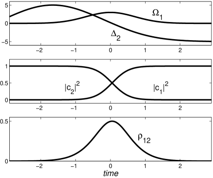
Figure 2: SCRAP procedure producing complete population transfer and a pulse of large atomic coherence. Time evolution of the detuning $\Delta_{2}$ and the two-photon Rabi frequency $\Omega_{1}$ (top frame), the populations of the $\left|1\right\rangle$ and $\left|2\right\rangle$ states (middle frame), and the coherence $\rho_{12}$ (bottom frame).

Fig. 2 shows the population and coherence dynamics induced in an atomic system driven by laser pulses in SCRAP configuration. As described above, population is transferred completely from the ground to the excited state, as the atomic transition frequency is swept in the falling edge of the Stark shifting laser pulse through resonance with the pump laser (middle frame). The coherence $\rho_{12}$ induced in the system during the interaction reaches a maximum of $1/2$ when the population is distributed equally between the bare states $\left|1\right\rangle$ and $\left|2\right\rangle$. The system is prepared in maximum coherence. This happens, however, only at one instant of time, which results in a pulse of large atomic coherence $\rho_{12}\left(t\right)$. We note that the transient large coherence $\rho_{12}$ occurs also when the pump and Stark shifting laser pulses coincide. As we show later, however, such regime leads to quite low overal conversion efficiency due to phase matching reasons.

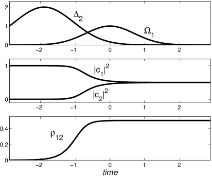
Figure 3: ”Half-SCRAP” procedure leading to a permanent coherence after the interaction. Time evolution of the detuning $\Delta_{2}$ and the two-photon Rabi frequency $\Omega_{1}$ (top frame), the populations of the $\left|1\right\rangle$ and $\left|2\right\rangle$ states (middle frame), and the coherence $\rho_{12}$ (bottom frame).

While the coherence, induced by SCRAP, is not permanent, a slight modification of the process permits the preparation of a long lasting maximum coherence (so called half-SCRAP) h-scrap . In this configuration the pump laser is tuned to resonance, i.e. the static detuning $\delta_{20}=0$. Fig. 3 shows the population dynamics and the coherence induced in this case. At earlier times we have $\Delta_{2}\gg\Omega_{1}$ so that the state $\left|\psi_{0}\right\rangle$ coincides with the ground state $\left|1\right\rangle$. When $\Omega_{1}$ increases, the adiabatic state $\left|\psi_{0}\right\rangle$ evolves in a superposition $\left|1\right\rangle$ and $\left|2\right\rangle$. At the end of the interaction the situation $\Omega_{1}\gg\left|\Delta_{2}\right|$ is reached, and the adiabatic state corresponds to ”maximum coherence”: $\left|\psi_{0}\right\rangle=\left(\left|1\right\rangle-\left|2\right\rangle\right)/\sqrt{2}$. This regime requires to fix the static detuning $\delta_{20}$ to zero with sufficient accuracy, but it establishes the enduring coherence needed for phase matching.

IV Hamiltonian approach formalism

In this work, we use an approach which does not require explicit expressions for the atomic amplitudes mel79 ; kryz ; kors02 .The main advantage of this approach is the reduction of Maxwell propagation equations (2) to the form of canonical Hamilton equations of classical mechanics involving action and angle variables $J$ and $\varphi$ (see Appendix). Here $\varphi$ is the relative phase of e.m. waves, Eq. (28), and the variable $J(z)$ characterizes the amount of energy exchange between the waves and has the initial condition $J(z=0)=0$:

$$\eta_{1}(z) = \eta_{10}-2J(z),$$

$$\eta_{2}(z) = \eta_{20}+J(z),$$ (31)

$$\eta_{3}(z) = \eta_{30}+J(z).$$

After some algebra (see Appendix), the Hamilton equations can be further reduced to yield an implicit solution for $J(z)$:

$$\pm\frac{N}{2}z=\int\limits_{0}^{J}S(J^{\prime})\frac{dJ^{\prime}}{\sqrt{R\left(J^{\prime}\right)}},$$ (32)

where both functions $R\left(J\right)$ and $S\left(J\right)$ are polynomials in $J$.

For the generation of the $\omega_{3}$ mode from vacuum: $\eta_{30}=0$, the functions $R\left(J\right)$ and $S\left(J\right)$ take a form:

$$R = 4\mu_{1}^{2}\mu_{2}\mu_{3}J\left(\eta_{10}-J\right)^{2}\left(\eta_{20}+J\right)$$

$$-\left(A_{1}+A_{2}J+A_{3}J^{2}\right)^{2}J^{2},$$

$$S = a_{0}+a_{1}J+a_{2}J^{2}.$$ (34)

As shown in the Appendix, cf. Eq. (97), the coefficients $A_{m}$ and $a_{m}$ describe the linear and nonlinear refraction coefficients of the medium.

Equation (32) matches a one-dimensional finite motion of a pendulum in an external potential. The allowed range of $J$, corresponding to the region of classically allowed motion of the pendulum, lies between $zero$ and the smallest positive root $J_{1}$ of the polynomial equation:

$$R\left(J\right)=0.$$ (35)

The second term in expression (IV) for $R\left(J\right)$ is never positive, so the smallest positive root of the polynomial is bounded by $\eta_{10}$. This reflects the fact that the conversion process stops when the energy of the pump field is entirely depleted. In order to reach this limit and thus to attain maximum conversion efficiency, the second term in (IV) should be small, which corresponds to negligible phase mismatch :

$$A_{1}+A_{2}J+A_{3}J^{2}\approx 0.$$

In order to see which values are required to approximately satisfy this condition, we have to analyze the coefficients $A_{m}$.

The coherence preparation process requires large static detuning $\delta_{30}$ and small ac Stark shift induced by the idler $\omega_{2}$ wave: $\mu_{2}\eta_{20}/\delta_{30}\ll\mu_{1}\eta_{10}$ (see discussion in Sec. III.C). Taking into account the relation $\mu_{2}/\mu_{1}\gg\delta_{30}$, Eq. (23), the latter requirement restricts the intensity of the $\omega_{2}$ wave: $\eta_{20}\ll\eta_{10}$. Since in the down-conversion process considered here the energy is taken only from the $\omega_{1}$ wave, this condition does not impose a real limitation.

Under these conditions, the non-vanishing coefficients $A_{m}$ and $a_{m}$ are given by

$$A_{1} \simeq -q\delta_{30}\left(2\lambda+\delta_{2}+\beta_{21}\eta_{10}\right)$$

$$-\mu_{2}\lambda-\mu_{3}\left(\lambda+\delta_{2}+\beta_{21}\eta_{10}\right),$$

$$A_{2} \simeq q^{2}\delta_{30}+\mu_{2}q+\mu_{3}\left(q-\beta_{22}-\beta_{23}+2\beta_{21}\right),$$ (37)

$$a_{0} \simeq \delta_{30}\left(2\lambda+\delta_{2}+\beta_{21}\eta_{10}\right),$$ (38)

$$a_{1} \simeq -\left(\mu_{2}+\mu_{3}\right),$$ (39)

where

$$q=2\Delta k/N$$ (40)

The eigenvalue $\lambda$ is a constant of motion which can thus be found from Eq. (96):

$$\lambda = \lambda_{0}=-\frac{1}{2}\left(\delta_{2}+\beta_{21}\eta_{10}\right)$$ (41)

$$+\frac{1}{2}\sqrt{\left(\delta_{2}+\beta_{21}\eta_{10}\right)^{2}+4\mu_{1}^{2}\eta_{10}^{2}}.$$

V Solutions for undepleted pump field

We first consider the solution of Eq. (32) for small density-length products $Nz$ in the case of low conversion efficiencies, i.e. the intensity of the generated field is assumed to be much smaller than the intensity of the pump $\omega_{1}$ wave:

$$\eta_{3}=J\ll\eta_{10}.$$

We can then neglect the term $A_{2}J$ in expression (IV), and the term $a_{1}J$ in expression (34). In this case the solution of Eq. (32) has a simple form:

$$\eta_{3}(z) = \frac{\eta_{20}}{1-\left(\frac{\Delta k^{\prime}}{2\kappa}\right)^{2}}\,\,\sinh^{2}\left(\kappa z\sqrt{1-\left(\frac{\Delta k^{\prime}}{2\kappa}\right)^{2}}\right),$$ (42)

$$\kappa = \frac{N}{2}\frac{\sqrt{\mu_{2}\mu_{3}}}{\delta_{30}}\frac{\mu_{1}\eta_{10}}{2\lambda+\delta_{2}+\beta_{21}\eta_{10}},$$ (43)

$$\Delta k^{\prime} = -\frac{N}{2}\frac{A_{1}}{a_{0}}$$ (44)

$$= \Delta k+\frac{N}{2}\frac{\mu_{3}\left(\lambda+\delta_{2}+\beta_{21}\eta_{10}\right)+\mu_{2}\lambda}{\delta_{30}\left(2\lambda+\delta_{2}+\beta_{21}\eta_{10}\right)},$$

which is similar to Eq. (11) obtained under the assumption of constant probability amplitudes of the states $|1\rangle$ and $|2\rangle$ (cf. Sect. II).

The optimum conversion (parametric gain with large rate $\kappa$) occurs when the phase mismatch $\Delta k^{\prime}$ is compensated. Taking into account Eq. (41) for $\lambda$, the condition for phase matching reads:

$$\frac{2}{N}\Delta k = -\frac{\mu_{3}+\mu_{2}}{2\delta_{30}}$$ (45)

$$-\frac{\mu_{3}-\mu_{2}}{2\delta_{30}}\frac{\left(\delta_{2}+\beta_{21}\eta_{10}\right)}{\sqrt{\left(\delta_{2}+\beta_{21}\eta_{10}\right)^{2}+4\mu_{1}^{2}\eta_{10}^{2}}}.$$

It is very important to recognize that the parameters $\delta_{2}$ and $\eta_{10}$ are time-dependent (pulsed) in the SCRAP process. Therefore, the r.h.s. of Eq. (45) is time-dependent. Hence, it is impossible to phase-match the generated and the pump waves for the duration of all stages of the light-atom interaction process. This fact has a detrimental effect for the full SCRAP procedure where the pulse of large coherence is produced (see discussion in Sec. III.C and Fig. 2). However, in the half-SCRAP case with the permanent large coherence (Fig. 3), there are two relatively long time intervals, in which the phase matching condition does not depend on time.

At the early stage of the SCRAP process, when $\delta_{2}\gg\mu_{1}\eta_{10}$, the condition is:

$$\frac{2}{N}\Delta k\approx-\frac{\mu_{3}}{\delta_{30}},$$ (46)

and the nonlinear conversion coefficient takes the form:

$$\kappa_{1}\approx\kappa_{0}\frac{\mu_{1}\eta_{10}}{\delta_{2}},$$ (47)

with the ”maximum coherence” conversion coefficient $\kappa_{0}$:

$$\kappa_{0}=\frac{N}{2}\frac{\sqrt{\mu_{2}\mu_{3}}}{\delta_{30}}.$$ (48)

For later times, when the Rabi frequency of the pump field exceeds the detuning: $\mu_{1}\eta_{10}\gg\delta_{2}$ and the adiabatic state corresponds to the maximum coherence superposition, the phase matching condition becomes:

$$\frac{2}{N}\Delta k=-\frac{\mu_{3}+\mu_{2}}{2\delta_{30}}-\frac{\mu_{3}-\mu_{2}}{2\delta_{30}}\frac{\beta_{21}}{\sqrt{\beta_{21}^{2}+4\mu_{1}^{2}}},$$ (49)

and the conversion coefficient is

$$\kappa_{2}\approx\kappa_{0}\frac{\mu_{1}}{\sqrt{\beta_{21}^{2}+4\mu_{1}^{2}}}.$$ (50)

Phase matching according to Eqs. (46), (49) can be performed by controlling the background mismatch $\Delta k$ through a suitable choice of the small angle of the $\omega_{2}$ wave propagation direction from the $z$-axis. For radiation in the visible spectral range, detuning $\delta_{30}\sim$100 GHz and atom densities $N\sim 10^{13}\div 10^{14}$ $cm^{-3}$, the value of $\Delta k$ necessary to compensate the resonance refraction contributions, Eqs. (46), (49), corresponds to an angle of $0.1-1$ $mrad$.

It is obvious from Eqs. (47), (50) that $\kappa_{2}\gg\kappa_{1}$. Therefore, it is advantageous to drive the frequency conversion process when a large coherence is established, thus to apply the pulse at $\omega_{2}$ when $\mu_{1}\eta_{10}\gg\delta_{2}$ and to choose parameters satisfying the condition Eq. (49).

When phase matching is not maintained, the quantity $1-\left(\Delta k^{\prime}/2\kappa\right)^{2}$ is always negative ($\Delta k$ is much smaller than the resonant contributions to $\Delta k^{\prime}$), and there is no exponential growth but sinusoidal oscillations of the generated intensity with respect to $Nz$. However, for $\mu_{1}\eta_{10}\gg\delta_{2}$ (maximum coherence) the quantity $\left|1-\left(\Delta k^{\prime}/2\kappa\right)^{2}\right|$ in the denominator of Eq. (42) is of the order of unity, whereas for $\delta_{2}\gg\mu_{1}\eta_{10}$ (atoms are in the ground state) we have $\left|1-\left(\Delta k^{\prime}/2\kappa\right)^{2}\right|\sim\left(\Delta k^{\prime}/2\kappa\right)^{2}\gg 1$, and correspondingly, conversion is tiny.

These considerations, similar to those of Sect. II treating the nonlinear conversion with fixed probability amplitudes, demonstrate once again that large atomic coherence is preferable whatever the method of the preparation might be.

Thus, in the case of good phase matching, we observe exponential growth of the generated intensity. The question arises up to which values the generated intensity will grow and what the limiting factors are? Since the pump wave will be depleted, one may also expect that the preparation of large atomic coherence will not be efficient anymore. By then it is not clear how this will influence the frequency conversion process. In order to answer these questions we need to solve the complete propagation problem taking into account the depletion of the pump field.

VI General solutions for resonant four-wave mixing

The solution of the propagation equation (32) is determined by the roots of cubic equation (35), in particular, by their signs and relation between their modules. Under the condition $\eta_{20}\ll\eta_{10}$, the roots of (35) can be well approximated by:

$$x_{1} = \frac{1-b_{1}}{1+b_{2}},$$ (51)

$$x_{2} = \frac{1+b_{1}}{1-b_{2}},$$ (52)

$$x_{3} = -\frac{\eta_{20}}{\eta_{10}}\frac{1}{1-b_{1}^{2}},$$ (53)

where

$$x_{j}=\frac{J_{j}}{\eta_{10}}.$$

The quantities $b_{1},b_{2}$:

$$b_{1} = \frac{A_{1}}{2\mu_{1}\eta_{10}\sqrt{\mu_{2}\mu_{3}}},$$

$$b_{2} = \frac{A_{2}}{2\mu_{1}\sqrt{\mu_{2}\mu_{3}}}$$

determine the phase mismatch induced by linear refraction and Kerr effect, respectively.

Since $\eta_{20}/\eta_{10}\ll 1$ we have in most relevant cases: $\left|x_{3}\right|\ll\left|x_{1}\right|,\left|x_{2}\right|$.

Evaluation of the integral in Eq. (32) gives the following general dependence for $x(z)\equiv J\left(z\right)/\eta_{10}$ in implicit form:

$$\pm\kappa^{\prime}z+\chi_{0}=F\left[\gamma\left(x\right),p\right]$$

$$\quad-\frac{a_{1}\eta_{10}}{a_{0}}r\left\{F\left[\gamma\left(x\right),p\right]-d\Pi\left[\gamma\left(x\right),n,p\right]\right\},$$ (54)

where $\chi_{0}$ is an integration constant, and $F\left(\gamma,p\right)$ and $\Pi\left(\gamma,n,p\right)$ are the elliptic integrals of the first and third kind, respectively ell . $\kappa^{\prime}$ is the nonlinear conversion coefficient defined as

$$\kappa^{\prime}=\kappa_{0}\frac{\mu_{1}\eta_{10}\delta_{30}}{a_{0}}\sqrt{\left|1-b_{1}^{2}\right|\left(1+\frac{\left|x_{3}\right|}{\left|x_{1}\right|}\right)}\frac{1}{s}.$$ (55)

The parameters of the elliptic integrals $\gamma\left(x\right),n,p$ as well as the factors $r,s,d$ depend on the signs of expressions $\left(1-b_{1}^{2}\right)$ and $\left(1-b_{2}^{2}\right)$.

Due to the condition $\eta_{20}/\eta_{10}\ll 1$, the expression (54) can be inverted to give the explicit solutions presented below.

VI.1 Compensation of both linear refraction and Kerr effect : $b_{1}^{2}<1$ and $b_{2}^{2}<1$

For $b_{1}^{2}<1$ and $b_{2}^{2}<1$ the relevant parameters are:

$$\gamma\left(x\right) = \arcsin\sqrt{\frac{x\left(x_{1}+\left|x_{3}\right|\right)}{x_{1}\left(x+\left|x_{3}\right|\right)}},$$

$$p = \sqrt{\frac{x_{1}\left(x_{2}+\left|x_{3}\right|\right)}{x_{2}\left(x_{1}+\left|x_{3}\right|\right)}},\;n=\frac{x_{1}}{x_{1}+\left|x_{3}\right|},$$ (56)

$$d = 1,\quad s=1,\quad r=\left|x_{3}\right|.$$

In this case, the solution is as follows:

$$x\left(z\right)=\frac{x_{1}\left|x_{3}\right|\text{sn}^{2}\left[\kappa^{\prime}z;p\right]}{\left|x_{3}\right|+x_{1}\text{cn}^{2}\left[\kappa^{\prime}z;p\right]},$$ (57)

where sn$\left[\kappa z;p\right]$ and cn$\left[\kappa z;p\right]$ are the Jacobi elliptic sine and cosine functions, respectively ell .

In this case, the parameter $p$ is close to unity, so that sn$\left[\kappa z;p\right]\rightarrow\tanh\left(\kappa z\right)$ and cn$\left[\kappa z;p\right]\rightarrow$sech$\left(\kappa z\right)$. Thus, for small density-length products $Nz$ such that $\kappa^{\prime}z\ll\ln\left(x_{1}/\left|x_{3}\right|\right)$ the solution (57) is reduced to

$$x(z)=x_{3}\,\,\sinh^{2}\left(\kappa^{\prime}z\right),$$

which coincides exactly with the solution obtained under the condition of undepleted pump field, see Eq. (42).

For larger $Nz$, Eq. (57) has to be used. The form of this solution is shown by the solid line in Fig. 4. The maximum value of $x(z)$ attainable in this regime is given by $x_{1}$ corresponding to the intensity of the generated $\omega_{3}$ wave given by :

$$\left(\eta_{3}\right)_{max}=J_{max}=\eta_{10}\frac{1-b_{1}}{1+b_{2}},$$

which is of the order of $\eta_{10}$. Thus, almost complete conversion can be achieved in this regime. This maximum value is reached at the distance $z=\left(\kappa^{\prime}\right)^{-1}K\left(p\right)$ with $K\left(p\right)$ being a complete elliptic integral of the first kind, which can be approximated for $p\approx 1-\left|x_{3}\right|\left(x_{2}-x_{1}\right)/\left(x_{1}x_{2}\right)\rightarrow 1$ as

$$K\left(p\right)\approx\left(1/2\right)\ln\left(\frac{16x_{1}x_{2}}{\left(x_{2}-x_{1}\right)\left|x_{3}\right|}\right).$$

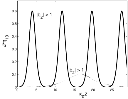
Figure 4: Spatial evolution of $J\left(z\right)$ at given retarded time $\tau$ in the case of compensated linear refraction. Parameters: $\eta_{20}/\eta_{10}=0.01$, $b_{1}=0.1$. The solid line corresponds to Eq. (57): $b_{2}=0.5$. The dotted line corresponds to Eq. (59): $b_{2}=8$, $s=5$.

VI.2 Compensation of linear refraction $b_{1}^{2}<1$, but large Kerr-induced refraction $b_{2}^{2}>1$

In this case, the parameters are as follows:

$$\gamma\left(x\right) = \arcsin\sqrt{\frac{\left|x_{2}\right|\left(x_{1}-x\right)}{x_{1}\left(x+\left|x_{2}\right|\right)}},$$

$$p = \sqrt{\frac{x_{1}\left(\left|x_{2}\right|-\left|x_{3}\right|\right)}{\left|x_{2}\right|\left(x_{1}+\left|x_{3}\right|\right)}},\;n=-\frac{x_{1}}{\left|x_{2}\right|},$$ (58)

$$d = 1-n,\quad s=1+\frac{a_{1}\eta_{10}}{a_{0}\sqrt{-n}},\quad r=\left|x_{2}\right|.$$

The solution reads :

$$x\left(z\right)=\frac{x_{1}\left|x_{3}\right|\text{sn}^{2}\left[\kappa^{\prime}z;p\right]}{\left|x_{3}\right|+x_{1}\frac{2\left|x_{2}\right|}{x_{1}+\left|x_{2}\right|}\text{cn}^{2}\left[\kappa^{\prime}z;p\right]},$$ (59)

The form of the solution is similar to the previous case, except for the prefactor at the cn${}^{2}\left[\kappa^{\prime}z;p\right]$ function in the denominator. The spatial evolution of the generated intensity in this case is plotted as a dotted line in Fig. 4.

We observe a parametric gain at the initial stage of the propagation, at $\kappa^{\prime}z\ll\ln\left(\frac{x_{1}}{\left|x_{3}\right|}\frac{\left|x_{2}\right|}{x_{1}+\left|x_{2}\right|}\right)$:

$$x(z)=x_{3}\,\,\frac{x_{1}+\left|x_{2}\right|}{2\left|x_{2}\right|}\sinh^{2}\left(\kappa^{\prime}z\right).$$ (60)

The maximum of $x(z)$ from Eq. (59) is again given by $x_{1}$. However, for large ”Kerr coefficient” $b_{2}\gg 1$, the value of $x_{1}$ corresponds to an intensity of the generated $\omega_{3}$ wave that is much smaller than $\eta_{10}$:

$$\left(\eta_{3}\right)_{max}\sim\frac{\eta_{10}}{b_{2}}.$$ (61)

It is also important to note that the conversion coefficient $\kappa^{\prime}$ here is smaller than in the ”compensated case” by a factor of $s\sim\left(\mu_{2,3}/\mu_{1}\delta_{30}\sqrt{-n}\right)\gg 1$. Therefore, the conversion proceeds much slower, see Fig. 4.

VI.3 No compensation of linear refraction : $b_{1}^{2}>1$

For $b_{1}^{2}>1$ and $b_{2}^{2}<1$ the elliptic integral parameters are:

$$\gamma\left(x\right) = \arcsin\sqrt{\frac{x\left(x_{3}+\left|x_{1}\right|\right)}{x_{3}\left(x+\left|x_{1}\right|\right)}},$$

$$p = \sqrt{\frac{x_{3}\left(x_{2}+\left|x_{1}\right|\right)}{x_{2}\left(x_{3}+\left|x_{1}\right|\right)}},\;n=\frac{x_{3}}{x_{3}+\left|x_{1}\right|},$$ (62)

$$d = 1,\quad s=1,\quad r=\left|x_{1}\right|.$$

For $b_{1}^{2}>1$ and $b_{2}^{2}<1$ :

$$\gamma\left(x\right) = \arcsin\sqrt{\frac{\left|x_{2}\right|\left(x_{3}-x\right)}{x_{3}\left(x+\left|x_{2}\right|\right)}},$$

$$p = \sqrt{\frac{x_{3}\left(\left|x_{2}\right|-\left|x_{1}\right|\right)}{\left|x_{2}\right|\left(x_{3}+\left|x_{1}\right|\right)}},\;n=-\frac{x_{3}}{\left|x_{2}\right|},$$ (63)

$$d = 1-n,\quad s=1,\quad r=\left|x_{2}\right|.$$

In both cases $p\ll 1$ and $n\ll 1$. This permits a reduction of the solution to the form:

$$x\left(z\right)=\left|x_{3}\right|\sin^{2}\left(\kappa^{\prime}z\right).$$ (64)

The maximum of $x\left(z\right)$ is $\left|x_{3}\right|$, i.e. $J_{max}=\eta_{20}/\left|1-b_{1}^{2}\right|$. Therefore, this solution demonstrates the crucial influence of the phase mismatch induced by linear refraction. If this contribution to the phase mismatch is not compensated, the maximum intensity of the generated $\omega_{3}$ wave is always limited by the input intensity $\eta_{20}$ of the idler wave.

VII Compensation of phase mismatch

As we have shown in the previous section, it is crucial to compensate the mismatch induced by linear refraction $b_{1}^{2}<1$ in order to get large conversion. Only then exponential gain occurs at the initial stage of the process and the maximum generated intensity will be much larger than the input intensity $\eta_{20}$ of the idler $\omega_{2}$ wave. At the same time, it is desirable to make the Kerr-induced mismatch as small as possible.

VII.1 Compensation of the phase mismatch induced by linear refraction

In general, the condition $b_{1}^{2}<1$ yields :

$$y_{0}-\frac{1}{\sqrt{1+d_{2}^{2}}}<y<y_{0}+\frac{1}{\sqrt{1+d_{2}^{2}}},$$ (65)

where the ”phase-matching-tuning parameter” $y$ is:

$$y\equiv\frac{q\delta_{30}}{\sqrt{\mu_{2}\mu_{3}}}.$$ (66)

The value of $y_{0}$:

$$y_{0}=-\frac{1-m}{2\sqrt{m}}\frac{d_{2}}{\sqrt{1+d_{2}^{2}}}-\frac{1+m}{2\sqrt{m}}\quad\left(y_{0}<0\right),$$ (67)

with notations

$$m = \frac{\mu_{2}}{\mu_{3}},$$ (68)

$$d_{2} = \frac{\beta_{21}}{2\mu_{1}}+\frac{\delta_{2}}{2\mu_{1}\eta_{10}},$$ (69)

corresponds to the condition given by Eq. (45) where $b_{1}=0$ (complete compensation of the linear refraction).

At the limits

$$y_{1,2}=y_{0}\mp 1/\sqrt{1+d_{2}^{2}}$$ (70)

of the desirable range of $y$, we have $b_{1}\rightarrow\pm 1$. From Eqs. (51)-(53) we see that the root $x_{1}$ determining the maximum conversion efficiency becomes very small at these values of $y$. Therefore, it is not favorable to set the working point close to $y_{1,2}$.

We stress an important consequence of the inequality (65): For any $\delta_{2}$ and $\mu_{1}\eta_{10}$, the quantity $y<0$ as well as its absolute value is of the order of one: $\left|y\right|\sim 1$ in the range given by Eq. (65). Therefore, $q\sim\mu_{2,3}/\delta_{30}$ and

$$\left|b_{2}\right|\sim\frac{\mu_{2,3}}{\mu_{1}\delta_{30}}\gg 1.$$

The Kerr-induced phase mismatch is large in the range of parameters ($q$ and $\delta_{30}$) while linear refraction is compensated in this regime. Thus it seems impossible to simultaneously compensate both contributions of the phase mismatch.

VII.2 Compensation of the phase mismatch induced by the Kerr effect

Condition $b_{2}^{2}<1$ yields :

$$\left|y\left(y+\frac{1+m}{\sqrt{m}}\right)\right|<\frac{2\mu_{1}\delta_{30}}{\sqrt{\mu_{2}\mu_{3}}}.$$ (71)

Due to $2\mu_{1}\delta_{30}/\sqrt{\mu_{2}\mu_{3}}\ll 1$, the above condition can be fulfilled by

$$\left|y\right|<\frac{2\mu_{1}\delta_{30}}{\mu_{2}+\mu_{3}}\quad\left(\ll 1\right),$$ (72)

i.e., by $y\approx y_{3}=0$ (or equivalently, by $q\approx 0$), and by

$$\left|y+\frac{1+m}{\sqrt{m}}\right|<\frac{2\mu_{1}\delta_{30}}{\sqrt{\mu_{2}\mu_{3}}},$$ (73)

that is by $y\approx y_{4}=-\left(1+m\right)/\sqrt{m}$ [or equivalently, by $q\delta_{30}\approx-\left(\mu_{2}+\mu_{3}\right)$, see Eq. (49)] in a very small range $\pm 2\mu_{1}\delta_{30}/\left(\mu_{2}+\mu_{3}\right)$. The values for $y_{3,4}$ are fixed by atomic parameters and cannot be tuned.

Further, it is easy to show that

$$y_{4}\leq y_{1}<y_{2}<0.$$ (74)

We see that the only possibility to satisfy both $b_{1}^{2}<1$ and $b_{2}^{2}<1$ is to make the value $y_{1}$ close to $y_{m}$ and to tune $y$ to the vicinity of $y_{1}$ (and $y_{m}$). However, as we have discussed in the previous subsection, it is not favorable to work with $y$ close to $y_{1}$ since the root $x_{1}$, which determines the maximum conversion, becomes very small. Moreover, the condition $y_{1}=y_{m}$ reduces to

$$d_{2}=\frac{\left(1-m\right)}{2\sqrt{m}},$$ (75)

what can be realized only at one instant of time, because $d_{2}$ is a time-dependent function, see Eq. (69). Then, only a very narrow part of the generated pulse may, in principle, be phase-matched to the pump waves, and any small deviation from the above condition given by Eq. (75) will destroy the phase matching.

VIII Spatio-temporal evolution. Total conversion efficiency

As we have seen before, there are different phase matching regimes at different stages of the SCRAP process. If we choose to compensate the linear refraction by satisfying the relationship (49), then at the beginning when $\delta_{2}\gg\mu_{1}\eta_{10}$ the linear refraction is large: $\left|b_{1}\right|>1$. When the pump intensity reaches the values $\mu_{1}\eta_{10}$ $\gg\delta_{2}$ the mismatch is completely compensated. Therefore, it is favorable to start the conversion process, i.e., to apply $\omega_{2}$ pulse at time instants when $\mu_{1}\eta_{10}$ $\gg\delta_{2}$. However, the delay of $\omega_{2}$ pulse should not be too large since the conversion process is also determined by the overlap between the pump $\omega_{1}$ and the idler $\omega_{2}$ pulses. In order to illustrate these processes, we show graphical representation of our analytical results in Figs. 5, 6, 7. Figs. 5 and 6 demonstrate the evolution of the generated intensity in the case of the permanent coherence preparation by the half-SCRAP, and Fig. 7 - for the case of pulsed large atomic coherence induced during the population transfer in the full SCRAP process.

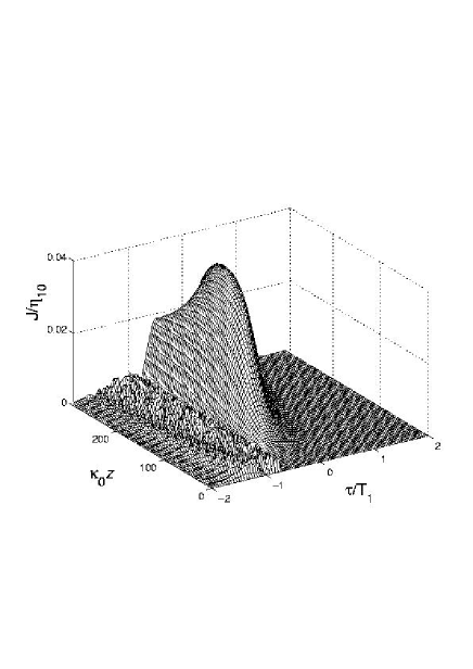
Figure 5: Spatio-temporal evolution of generated intensity $J\left(z,\tau\right)$ (normalized to the maximum of $\eta_{10}$) for the half-SCRAP preparation and linear refraction compensation at maximum coherence according to Eq. (49). The retarded time $\tau$ is in units of the duration $T_{1}$ of the pump $\omega_{1}$ pulse, and the propagation distance $z$ is in units of conversion length $\kappa_{0}^{-1}$ for the ideal maximum coherence case, Eq. (48). The parameters are $\mu_{2}/\mu_{3}=7.95$, $\beta_{21}/2\mu_{1}=0.1$ (Kr atoms), $\mu_{2}/\left(2\mu_{1}\delta_{30}\right)=20$. The temporal profile of the Stark, pump and idler pulse is Gaussian with the following parameters: maximum of detuning and pump Rabi frequency: $\delta_{2}^{m}/\Omega_{10}^{m}=2$, static detuning $\delta_{20}=0$, $\eta_{20}^{m}/\eta_{10}^{m}=0.005$, center of the Stark pulse $t_{s}/T_{1}=-1.5$, duration of the Stark pulse $T_{s}/T_{1}=1$, duration of the $\omega_{2}$ pulse $T_{2}/T_{1}=0.5$, delay of the $\omega_{2}$ pulse $t_{2}/T_{1}=-1$.

In Fig. 5, with the idler $\omega_{2}$ pulse arriving before the pump $\omega_{1}$ pulse, sinusoidal oscillations occure along the propagation path for the early part of the generated pulse. This corresponds to Eq. (64) for the case of uncompensated phase mismatch. As the pump intensity $\eta_{10}$ increases and the interaction parameters get closer to the phase matching condition Eq. (49) and $\left|b_{1}\right|$ becomes sufficiently small: $\left|b_{1}\right|<1$, Eq. (59) is applied. During this time interval intensities $J$ much larger than $\eta_{20}$ do occur. We recall that $\eta_{20}$ is the maximum intensity that can be obtained without elimination of linear refraction. However, since the Kerr-induced mismatch is large, the maximum generated intensity $\eta_{3}=J$ is still much smaller than $\eta_{10}$ (it is given by $\eta_{10}/b_{2},$ Eq. (61)), and the rate of intensity growth is quite small.

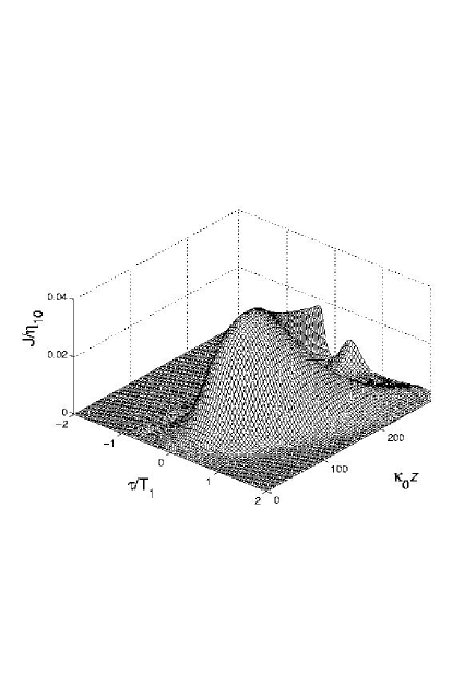
Figure 6: Evolution of $J\left(z,\tau\right)$ for the half-SCRAP preparation and compensation of linear refraction at maximum coherence by Eq. (49). Parameters are the same as in Fig. 5 except the delay of the $\omega_{2}$ pulse $t_{2}/T_{1}=0$. For better visibility, the time and length axes have been reversed as compared to Fig. 5.

Fig. 6 shows the variation of the intensity $J$ with $\tau$ and $z$, when the phase matching takes place over the entire duration of the generated pulse. We see from Figs. 5, 6 that the maximum of the generated pulse always coincides with the maximum of the pump $\omega_{1}$ pulse and not with that of the idler $\omega_{2}$ pulse. This fact directly follows from the physics of the down-conversion process in which the $\omega_{2}$ field serves simply as a seed wave, while the energy is taken only from the pump $\omega_{1}$ field. However, the temporal overlap between the pump and the idler pulses also influences the conversion process. Initially, there is exponential growth with $x(z)\sim x_{3}\sinh^{2}\left(\kappa^{\prime}z\right)\sim\eta_{20}/\eta_{10}$, Eq. (60). Thus the generated intensity is determined mainly by the idler field: $\eta_{3}\sim\eta_{20}\sinh^{2}\left(\kappa^{\prime}z\right)$. Later, the maximum of the generated pulse is shifted towards the maximum of the $\omega_{1}$ pulse. This dynamics leads, in general, to a temporal modulation of the generated pulse. The best conditions are obtained when the maxima of the pump $\omega_{1}$ and the idler $\omega_{2}$ pulses coincide (Fig. 6). In this case, conversion proceeds more or less homogeneously and the temporal shape of the generated pulse is smooth at all propagation distances.

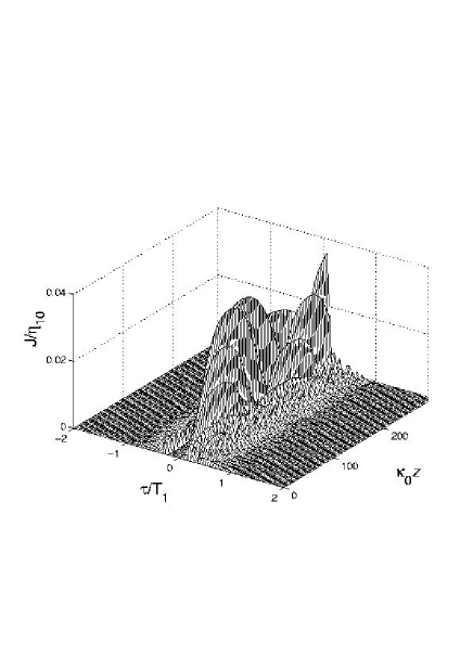
Figure 7: Evolution of $J\left(z,\tau\right)$ for the temporally large coherence induced during the full SCRAP process. Linear refraction is compensated for maximum coherence by Eq. (49). Parameters are: $\delta_{2}^{m}/\Omega_{10}^{m}=10$, $\delta_{20}/\Omega_{10}^{m}=-5$, $t_{s}/T_{1}=-1.7$, $T_{s}/T_{1}=2$, $t_{2}/T_{1}=0$. Other parameters are the same as in Fig. 5. For better visibility, the time and length axes have been reversed as compared to Fig. 5.

When the large atomic coherence persists only in transient during the full SCRAP process, efficient generation occurs during a short time interval around the maximum of the pump pulse (see Fig. 7). This interval is determined by the range where the phase matching, $\left|b_{1}\right|<1$ , occurs.

As we see, the temporal shape of the generated pulse is in general quite complicated. That is the output pulse is not transform-limited. An important quantity to characterize the conversion process is the total energy conversion efficiency, defined as

$$W(z)\equiv\frac{\displaystyle{\int\mathrm{d}t\,\omega_{3}\eta_{3}(z,t)}}{\displaystyle{\ \int\mathrm{d}t\,\omega_{1}\eta_{10}(z,t)}}.$$ (76)

The evolution of $W(z)$ is shown in Fig. 8 for three different delays of the idler pulse in the case of permanent coherence. The largest conversion efficiency is obtained for coinciding $\omega_{1}$ and $\omega_{2}$ pulses. Moreover, the maximum of $W(z)$ occurs at propagation distances smaller than that for the case of delayed pulses. However, the total conversion efficiency is not substantially different for different delays because the maximum of $W(z)$ is determined mainly by $\eta_{10}^{m}/b_{2}$ , i.e., by the parameters of the pump pulse. The thin solid line in Fig. 8 displays the conversion efficiency in the case of pulsed large coherence. As expected, the efficiency is much smaller than in the ”permanent $\rho_{12}$” case because of two reasons. First, the nonlinear conversion coefficient $\kappa$, Eq. (12), is large in the transient regime during a short time slot. Second, more important, phase matching, as discussed above, can be achieved only in an even shorter time interval.

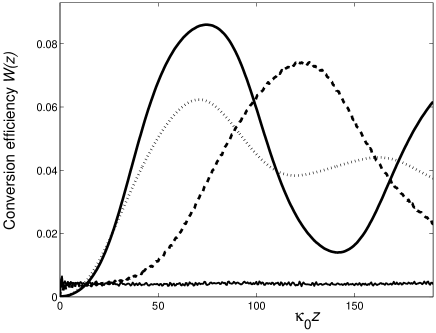
Figure 8: Spatial dependence of the total conversion efficiency $W$, Eq. (76), for different delays of the $\omega_{2}$ pulse for the half-SCRAP coherence preparation: solid line - $t_{2}/T_{1}=0$, dotted line - $t_{2}/T_{1}=+1$, dashed line - $t_{2}/T_{1}=-1$. The values for all other parameters are the same as in Fig. 5. The lower thin solid line corresponds to the transient large coherence induced during the full SCRAP process, Fig. 7.

IX Conclusions

We have discussed the analytic solutions of a four-wave mixing process involving preparation of an atomic system driven to maximum coherence by the technique of Stark chirped rapid adiabatic passage (SCRAP). The maximum coherence permits conversion efficiencies, exceeding the case of conventional nonlinear optics by a large factor. However, the conversion efficiency does not reach unity, because of phase mismatch due to the linear and the intensity-dependent index of refraction. It is practically impossible to compensate both parts simultaneously. Thus, the conversion efficiency gets maximum when the linear part of the phase mismatch is reduced to zero. This can be done by the controlling the residual phase mismatch $\Delta k$ through the buffer gas or non-collinear pulse propagation. Unfortunately, the Kerr-induced mismatch is large and limits the rate and the maximum achievable efficiency of the conversion. Still the maximum atomic coherence, prepared by SCRAP, permits efficient generation of strong short-wavelength radiation. In principle, the generated radiation is broadly tunable - the detuning $\delta_{30}$ may be changed provided it is still larger than Rabi frequencies and ac Stark shifts. However, the phase matching condition Eq. (49) has to be satisfied. Therefore, tuning of $\delta_{30}$ requires modified compensation of the residual phase mismatch $\Delta k$.

X Acknowledgments

We acknowledge support from the European Union, through the RTN COCOMO contract number HPRN-CT-1999-000129, the Deutsche Forschungsgemeinschaft (DFG) as well as the German-Israeli Foundation (GIF), contract number I-644-118.5/1999. The work of E.A.K. was supported by the Alexander von Humboldt Foundation. We would like to thank M. Fleischhauer for many useful discussions.

Appendix A Hamiltonian approach

Here we present an outline of the Hamiltonian approach in nonlinear optics mel79 ; kryz ; kors02 . This approach is based on the representation of the medium polarization $P$ as a partial derivative of the time-averaged free energy density of a dielectric with respect to the electric field strength $E$ LL :

$$P=-\left\langle N\frac{\partial\hat{H}}{\partial E}\right\rangle,$$ (77)

where $\left\langle...\right\rangle$ denotes quantum-mechanical averaging, and $\hat{H}$ is the single-atom interaction Hamiltonian. With the field given by Eq. (1), we write:

$$P=-\left\langle N\sum_{j}\frac{\partial\hat{H}}{\partial\mathcal{E}_{j}^{\ast}}\exp(-i(\omega_{j}t-k_{j}z))+c.c.\right\rangle,$$ (78)

thus the propagation equation (2) becomes:

$$\frac{\partial\mathcal{E}_{j}}{\partial z}=-i2\pi\frac{\omega_{j}}{c}N\left\langle\frac{\partial\hat{H}}{\partial\mathcal{E}_{j}^{\ast}}\right\rangle.$$ (79)

When the atomic system adiabatically follows the instantaneous eigenstate $\left|\psi_{0}\right\rangle$, we find

$$\left\langle\frac{\partial\hat{H}}{\partial\mathcal{E}_{j}^{\ast}}\right\rangle=\left\langle\psi_{0}\right|\frac{\partial\hat{H}}{\partial\mathcal{E}_{j}^{\ast}}\left|\psi_{0}\right\rangle=\hbar\frac{\partial\lambda_{0}}{\partial\mathcal{E}_{j}^{\ast}}.$$

Hence the propagation equation can be written as:

$$\frac{\partial\mathcal{E}_{j}}{\partial z}=-i2\pi\frac{\hbar\omega_{j}}{c}N\frac{\partial\lambda_{0}}{\partial\mathcal{E}_{j}^{\ast}}.$$ (80)

In the following discussion it is useful to express the field amplitude $\mathcal{E}_{j}$ in terms of photon flux $\eta_{j}$, Eq. (8), and phase $\varphi_{j}$. Separating the real and imaginary parts, we find from Eq. (80):

$$\frac{\partial\eta_{j}}{\partial z} = -\frac{\partial\mathcal{H}^{\prime}}{\partial\varphi_{j}},$$ (81)

$$\frac{\partial\varphi_{j}}{\partial z} = \frac{\partial\mathcal{H}^{\prime}}{\partial\eta_{j}}.$$

These equations have the form of Hamilton equations of classical canonical mechanics with action and angle variables $\eta_{j}$, and $\varphi_{j}$, ”time” $z$, and the Hamiltonian function $\mathcal{H}^{\prime}=\frac{1}{2}N\lambda_{0}$.

One can see from the eigenvalue equation (27) that $\lambda_{0}$ and, hence $\mathcal{H}^{\prime}$, depend on the field phases $\varphi_{j}$ only through the relative phase $\varphi$. Therefore, we have:

$$\frac{\partial\mathcal{H}^{\prime}}{\partial\varphi_{1}}=-2\frac{\partial\mathcal{H}^{\prime}}{\partial\varphi_{2}}=-2\frac{\partial\mathcal{H}^{\prime}}{\partial\varphi_{3}}\left(=2\frac{\partial\mathcal{H}^{\prime}}{\partial\varphi}\right).$$ (82)

An immediate consequence of this symmetry of $\mathcal{H}^{\prime}$ is the existence of constants of motion. Substituting the above equations (82) into the first line of Eqs. (81) yields the well-known Manley-Rowe relations boyd :

$$\frac{\partial\eta_{1}}{\partial z}=-2\frac{\partial\eta_{2}}{\partial z}=-2\frac{\partial\eta_{3}}{\partial z},$$ (83)

which correspond to two independent constants of motion:

$$\eta_{1}+2\eta_{3} = \eta_{10}+2\eta_{30},$$ (84)

$$\eta_{1}+2\eta_{2} = \eta_{10}+2\eta_{20}.$$

Here $\eta_{j0}=\eta_{j}(z=0)$ are the photon flux values at the entrance to the medium. Taking into account the multiphoton resonance condition (25), one finds furthermore that the total intensity of the elm. fields is conserved: $I_{1}+I_{2}+I_{3}=const(z)$. The relations Eq. (84) enable us to re-write $\eta_{j}$ as:

$$\eta_{1}(z) = \eta_{10}-2J(z),$$

$$\eta_{2}(z) = \eta_{20}+J(z),$$ (85)

$$\eta_{3}(z) = \eta_{30}+J(z).$$

The function $J(z)$ characterizes the amount of energy exchange between the waves and has the initial condition $J(z=0)=0$.

Thus the original problem with six amplitude and phase variables can be reduced to two variables $J$ and $\varphi$ by a canonical transformation. This leads to

$$\frac{\partial J}{\partial z} = -\frac{\partial\mathcal{H}}{\partial\varphi},$$ (86)

$$\frac{\partial\varphi}{\partial z} = \frac{\partial\mathcal{H}}{\partial J},$$ (87)

with new Hamiltonian function

$$\mathcal{H}=\frac{1}{2}N\lambda_{0}+\Delta kJ\equiv\frac{1}{2}N\lambda.$$ (88)

As can be seen from Eqs. (88) and (27), $\mathcal{H}$ (or $\lambda$) does not depend on the coordinate $z$ explicitly. Therefore, $\mathcal{H}$ (or $\lambda$) is a fourth constant of motion expressing the conservation of the energy density of the medium with respect to $z$.

To solve the remaining two equations of motion for $J(z)$ and $\varphi(z)$, the Rabi-frequencies $\Omega_{j}$ are expressed in terms of $\eta_{j0}$ and $J$, and the characteristic equation (27) is written in the form

$$G(\lambda,J)=g(J)\cos\varphi.$$ (89)

Differentiating both sides with respect to $\varphi$ yields

$$\frac{\partial G}{\partial\varphi}=\frac{\partial G}{\partial\lambda}\frac{\partial\lambda}{\partial\varphi}=-g\sin\varphi=\pm\sqrt{g^{2}-G^{2}}.$$

Substituting this relation into Eq. (86), we find:

$$\frac{\partial J}{\partial z}=\pm\frac{N}{2}\frac{\sqrt{g^{2}-G^{2}}}{\partial G/\partial\lambda}.$$ (90)

The choice of the sign in Eq. (90) depends on the sign of $\sin\varphi$ at $z=0$. Integration of Eq. (90) gives an implicit solution for $J(z)$:

$$\pm\frac{N}{2}z=\int\limits_{0}^{J}\frac{\partial G(J^{\prime})}{\partial\lambda}\frac{dJ^{\prime}}{\sqrt{g^{2}\left(J^{\prime}\right)-G^{2}\left(J^{\prime}\right)}}.$$ (91)

Both functions $g^{2}-G^{2}$ and $\partial G/\partial\lambda$ are polynomials in $J$:

$$g = -2\mu_{1}\sqrt{\mu_{2}\mu_{3}}$$

$$\times\sqrt{\left(\eta_{10}-2J\right)^{2}\left(\eta_{20}+J\right)\left(\eta_{30}+J\right)},$$

$$G = G_{0}+\sum_{m=1}^{3}A_{m}J^{m},$$ (93)

$$\frac{\partial G}{\partial\lambda} = \sum_{m=0}^{2}a_{m}J^{m}.$$ (94)

Therefore, equation (90) describes a one-dimensional finite motion of a pendulum in an external potential. The solution is in general given by some combination of elliptic functions ell with parameters determined mainly by the roots $J_{n}$ of the polynomial equation:

$$g^{2}\left(J\right)-G^{2}\left(J\right)=0.$$ (95)

The eigenvalue $\lambda$ is a constant of motion (cf. Eq. (88)), and can thus be found from the characteristic equation (89) with parameters taken at the medium entrance $z=0$:

$$G_{0}\left(\lambda\right)=g(z=0)\cos\varphi(z=0).$$ (96)

Thus, we have reduced the propagation problem to solving two algebraic equations: (96) for $\lambda$ and (95) for the roots $J_{n}$. If this can be done explicitly, the Hamiltonian method provides an analytical solution to the propagation problem. But even if an explicit solution is not possible, it considerably simplifies numerical calculations. The physical meaning of the coefficients $A_{m}$ and $a_{m}$ can be drawn by considering the canonical equation (87) for the relative phase:

$$\frac{\partial\varphi}{\partial z}=\frac{N}{2}\frac{\partial\lambda}{\partial J}=\frac{N}{2}\frac{\partial G/\partial J}{\partial G/\partial\lambda}=\frac{N}{2}\frac{A_{1}+2A_{2}J+3A_{3}J^{2}}{a_{0}+a_{1}J+a_{2}J^{2}}.$$ (97)

One recognizes that the $A_{m}$ and $a_{m}$ describe the linear and nonlinear refraction coefficients of the medium. E.g. if $J$ is sufficiently small, the first term $NA_{1}/2a_{0}$ on the right-hand side of Eq. (97) can be identified with the phase mismatch induced by the linear refraction, including both contributions from the three-level interaction and the residual mismatch $\Delta k$. The second term $\left(N/2a_{0}\right)\left(2A_{2}-a_{1}A_{1}/a_{0}\right)J$ in the expansion over $J$ corresponds to the phase mismatch due to Kerr effect, and the next terms are responsible for the higher-order contributions.

References

• (1) M. Jain, H. Xia, G.Y. Yin, A.J. Merriam, and S.E. Harris, Phys. Rev. Lett. 77, 4326 (1996); S.E. Harris, G.Y. Yin, M. Jain, H. Xia, and A.J. Merriam, Phil. Trans. R. Soc. Lond. A 355, 2291 (1997).
• (2) A.J. Merriam, S.J. Sharpe, H. Xia, D. Manuszak, G.Y. Yin, and S.E. Harris, Opt. Lett. 24, 625-627 (1999); IEEE Journal of Selected Topics in Quantum Electronics 5, 1502 (1999).
• (3) K. Bergmann, H. Theuer, and B. W. Shore, Rev. Mod. Phys. 70, 1003 (1998); N.V. Vitanov, M. Fleischhauer, B. W. Shore, and K. Bergmann, Adv. At. Mol. Opt. Phys. 46, 55 (2001).
• (4) L. P. Yatsenko, S. Guerin, T. Halfmann, K. Böhmer, B. W. Shore, and K. Bergmann, Phys. Rev. A 58, 4683 (1998); S. Guerin, L. P. Yatsenko, T. Halfmann, B. W. Shore, and K. Bergmann, Phys. Rev. A 58, 4691 (1998); K. Böhmer, T. Halfmann, L. P. Yatsenko, B.W. Shore, and K. Bergmann, Phys. Rev. A 64, 02340 (2001).
• (5) L.P. Yatsenko, B.W. Shore, T. Halfmann, K. Bergmann, and A. Vardi, Phys. Rev. A 60, R4237 (1999); T. Rickes, L.P. Yatsenko, S. Steuerwald, T. Halfmann, B.W. Shore, N.V. Vitanov, and K. Bergmann, J. Chem. Phys. 113, 534 (2000).
• (6) L.P. Yatsenko, N.V. Vitanov, B.W. Shore, T. Rickes, and K. Bergmann, Opt. Commun. 204, 413 (2002).
• (7) S.A. Myslivets, A.K. Popov, T. Halfmann, J.P. Marangos and T.F. George, Opt. Comm, 335 (2002).
• (8) A.O. Melikyan and S.G. Saakyan, Zh. Exp.Teor. Fiz. 76, 1530 (1979) [Sov. Phys. JETP 49, 776 (1979)].
• (9) A.R. Karapetyan and B.V. Kryzhanovskii, Zh. Exp. Teor. Fiz. 99, 1103 (1991) [Sov. Phys. JETP 72, 613 (1991)]; B. Kryzhanovsky and B. Glushko, Phys. Rev. A 45, 4979 (1992).
• (10) E.A. Korsunsky and M. Fleischhauer, Phys. Rev. A 66, 033808 (2002).
• (11) S.E. Harris and M. Jain, Opt. Lett. 18, 998-1000 (1993).
• (12) R.W. Boyd, Nonlinear optics, (Academic Press, San Diego, 1992).
• (13) C. Dorman and J.P. Marangos, Phys. Rev. A 58, 4121 (1998); C. Dorman, I. Kucukkara, and J.P. Marangos, Phys. Rev. A 61, 013802 (1999).
• (14) C. Dorman, I. Kucukkara, and J.P. Marangos, Opt. Commun. 180, 263 (2000).
• (15) P.F. Byrd and M.D. Friedman, Handbook of Elliptic Integrals for Engineers and Scientists (Springer, Berlin, 1971); Handbook of Mathematical Functions, ed. by M. Abramowitz and I.A. Stegun (Dover, New York, 1965).
• (16) L.D. Landau and E.M. Lifshitz, Electrodynamics of Continuous Media, (Pergamon Press, New York 1975).