Two photon interference and optical free induction decay

Abstract

The two photon interference phenomenon is theoretically investigated for the general situations with an arbitrary input two photon state with and without photon polarization. For the case without polarization, the necessary-sufficient condition for the destructive interference of coincidence counting is given as the symmetric pairing of photons in the light pulses. For both case it is shown that the ”dip” in coincidence curve can be understood in terms of the free induction decay mechanism. This observation predicts the destructive interference phenomenon to occur even for certain cases with separable input two photon state, but it can only be explained in terms of ”the two photon (not two photons )interference ”.

] In last two decades one of the most important progresses in quantum optics is the experimental demonstration of the Einstern-Podolsky-Rosen (EPR) [1] effect with the entangled photons. The creation of EPR entangled photons in a spontaneous parametric down conversion (SPDC [2]) not only implements the best test of Bell’s inequality [3] with fewer loopholes [4-6], but also lays foundations for some quantum information techniques [7]. This important progress has inspired people to reconsider the profound observation that “…photon… only interferes with itself. ”stated by Dirac in his famous book “The Principle of Quantum Mechanics ”[8].

Some interesting experiments of typical two photon interferometer seem to illustrate the existence of interference between two different photons since a curve of “dip”was observed in the rate of two photon coincidence[9-11]. However, a series of refined experimental setups [12-14] concluded that Dirac is correct. They argue that “a two photon (not two photons) can also only interfere with itself” [14] to account for the exotic interference phenomenon. In this argument the crucial conception is the two photon or bi-photon, the inseparable photon pair depicted by a EPR state. In fact, the naive idea of “destructive interference between the idler and signal photons” can not give a correct prediction for a two photon interference experiment “with three arms”.

If one believe that the idea of bi-photon is indeed necessary for all the two photon interference experiments, then two natural questions follow immediately : 1. Does there exist the separable pair of photons to give the destructive interference in the two photon coincidence counting rate? In this case the separable pair of photons can be implemented experimentally in the two independent pulses of photons. 2.If there is indeed a destructive interference for two independent pulses of photons, does it imply “interference between the idler and signal photons”?

I Two photon interference of Type I

In this paper the two questions will be answered in an universal framework by considering a general input two photon state

$$|\Psi\rangle=\int_{0}^{\infty}d\omega\int_{0}^{\infty}d\tilde{\omega}f(\omega,\tilde{\omega})a_{A}^{+}(\omega)a_{B}^{+}(\tilde{\omega})|0\rangle.$$ (1)

The schematic setup for this consideration is illustrated in figure 1:

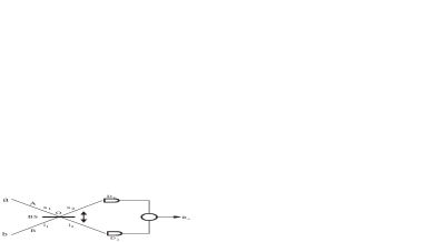
FIG. 1.: Schematic of the two-photon interferometer

the two lights coming from points $a$ and $b$ are mixed at point $O$ on the 50-50 beam splitter $BS$ and detected by the two photon counters at $D_{1}$ and $D_{2}$. Correspondingly, $a_{A}^{+}(\omega)$ ( $a_{B}^{+}(\tilde{\omega})$ ) is the creation operator for the photon of frequency $\omega$ ( $\tilde{\omega}$ ) in the optical path mode $A$ ($B)$ from the point $a$ $(b)$ to $O$; $f(\omega,\tilde{\omega})$ is the distribution function. The optical path modes can be regarded as the modes of idler and signal lights in the usual SPDC experiment with a special distribution function $f(\omega,\tilde{\omega})\propto$ $\delta(\omega+\tilde{\omega}-\omega_{0})$ for a finite real number $\omega_{0}.$ The separable pair of photons corresponds to the case with the factorized distribution function $f(\omega,\tilde{\omega})=f_{1}(\omega)f_{2}(\tilde{\omega}).$

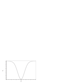
FIG. 2.: The destructive interference

With this configuration of gedankenexperiment, the above two questions can be asked in an unique way : what kind of two photon state (or what kind of distribution function $f(\omega,\tilde{\omega})$) can result in the curve of “dip” of the rate of two photon coincidence, which is illustrated in figures 2 as the typical destructive interference phenomenon. Here, $D=l_{1}-s_{1}$ is the optical path difference between $aO$ and $bO;$ $aO=$ $s_{1},bO=$ $l_{1},$ $D_{1}O=s_{2},$ $D_{2}O=l_{2}$ are the lengths of optical paths. The rate $R_{c}$ of coincident detection is measured as a function of the position of $BS$ and there is a ”null” in coincidence i.e., $R_{c}=0$ at $D=0$. This indicates a destructive interference. To explain the anti-exponential decaying behavior beside the ”dip” (or anti-peak) point, we will resort to the free induction decay mechanism [15].

In the following discussion we do not make assumptions about the light source, which may be the entangled photon pair created by the BBO nonlinear crystal or any two independent photon input pulse. We denote the positive frequency parts of the electric field at detectors $D_{1}$ and $D_{2}$ by $E_{1}^{+}$ and $E_{2}^{+}$. We will choose a proper position as the coordinate origin so that we could compute the coincidence rate conveniently. According to Glauber’s coherence theory [16,17], the probability per unit (time)² that one photon is recorded at $D_{1}$ at time $t_{1}$ and another at $D_{2}$ at time $t_{2}$ is just the second order coherence function.

$$G^{[2]}(t_{1},t_{2})=\langle\Psi|E_{2}^{-}(t_{2})E_{1}^{-}(t_{1})E_{1}^{+}(t_{1})E_{2}^{+}(t_{2})|\Psi\rangle$$ (2)

We recall that, when one consider the first order coherence the superposition of two obvious ”paths” is available. To describe the two particle interference phenomenon due to the second order coherence in a similar way, the generalized “path” is introduced by considering $G^{[2]}(t_{1},t_{2})=|\Psi(t_{1},t_{2})|^{2}$ where the bi-photon wave packet $\Psi(t_{1},t_{2})=\langle 0|E_{1}^{+}(t_{1})E_{2}^{+}(t_{2})|\Psi\rangle$ is invoked as a two photon effective wave-function [14]. Most recently this result was generalized for higher order coherence in time-domain [18]. Then, the two photon coincidence rate can be given by the two time integral $R_{c}=\int_{-\infty}^{\infty}dt_{1}dt_{2}|\Psi(t_{1},t_{2})|^{2}$.

In present discussion, in terms of the positive frequency part of the $A$ ($B$) mode electric field at point $a$ ($b$) with the spectral density $g(\omega)$

$$E_{a(b)}^{+}(\tau)=\int_{0}^{\infty}d\omega g(\omega)a_{A(B)}(\omega)e^{-i\omega\tau}$$ (3)

the local field operators

$$E_{1}^{+}(t_{1}) = \frac{1}{\sqrt{2}}[iE_{a}^{+}(\tau_{1})+E_{b}^{+}(\tau_{1}^{\prime})]$$ (4)

$$E_{2}^{+}(t_{2}) = \frac{1}{\sqrt{2}}[E_{a}^{+}(\tau_{2}^{\prime})+iE_{b}^{+}(\tau_{2})]$$ (5)

are implemented by the $50-50$ beam splitter with

$$\tau_{1} = t_{1}-\frac{s_{1}+s_{2}}{c},\tau_{2}=t_{2}-\frac{l_{1}+l_{2}}{c}$$

$$\tau_{1}^{\prime} = t_{1}-\frac{l_{1}+s_{2}}{c},\tau_{2}^{\prime}=t_{2}-\frac{s_{1}+l_{2}}{c}$$

where $c$ is the velocity of light. Then the two-photon wave function can be written explicitly as

$$\Psi=\int_{0}^{\infty}F\cdot[e^{-i(\tilde{\omega}\tau_{1}^{\prime}+\omega\tau_{2}^{\prime})}-e^{-i(\omega\tau_{1}+\tilde{\omega}\tau_{2})}]d\omega d\tilde{\omega}$$ (6)

with

$$F=F(\omega,\tilde{\omega})=\frac{1}{2}g(\omega)f(\omega,\tilde{\omega})g(\tilde{\omega}).$$ (7)

II The necessary-sufficient condition for the destructive coincidence

Now let’s prove that the necessary-sufficient condition for the destructive coincidence $R_{c}=0$ at $D=0$ is $f(\omega,\tilde{\omega})=$ $f(\tilde{\omega},\omega)$. To show the sufficience we decompose the two-photon wave packet $\Psi$ $=\Psi_{1}+\Psi_{2}$ into two parts

$$\Psi_{1} = \int_{0}^{\infty}d\omega d\tilde{\omega}F\cdot e^{-i(\omega\tau_{1}^{\prime}+\tilde{\omega}\tau_{2}^{\prime})}[1-e^{-i(\omega-\tilde{\omega})\frac{D}{C}}]$$ (8)

$$\Psi_{2} = \int_{0}^{\infty}d\omega d\tilde{\omega}G(\omega,\tilde{\omega})\cdot e^{-i(\omega\tau_{2}^{\prime}+\tilde{\omega}\tau_{1}^{\prime})}$$ (9)

where $G(\omega,\tilde{\omega})=F(\omega,\tilde{\omega})-F(\tilde{\omega},\omega)$ in the derivation, we have considered $\tau_{1}-\tau_{1}^{\prime}=\tau_{2}^{\prime}-\tau_{2}=\frac{D}{C}$. It is easy to see that $\Psi_{2}=0$ and $\Psi=\Psi_{1}$when $G(\omega,\tilde{\omega})=0$. On the other hand, $\Psi_{1}|_{D=0}=0$. Then, at $D=0$, $R_{c}=0.$ To show the necessity, we consider $|\Psi|^{2}=|\Psi_{1}|^{2}+|\Psi_{2}|^{2}+$ $2Re\Psi_{1}^{\ast}\Psi_{2}$. Since $\Psi_{1}=0$ at $D=0$ , $|\Psi|^{2}|_{D=0}=|\Psi_{2}|^{2}$. So if $R_{c}|_{D=0}=0$, then $|\Psi|^{2}|_{D=0}=|\Psi_{2}|^{2}=0$ i.e., $\Psi_{2}=0$. Because $G(\omega,\tilde{\omega})$ is the Fourier component of $\Psi_{2}$, the vanishing $\Psi_{2}$ must lead to $G=0$ or $f(\omega,\tilde{\omega})=f(\tilde{\omega},\omega)$.

In fact this necessary-sufficient condition proved above has been implied in several discussions [19-22].

To illustrate the main idea of  physics implied by the above proof, we consider the simplest symmetric state $|\Psi\rangle=|S(\Omega,\tilde{\Omega})\rangle$ $\equiv$ $\frac{1}{\sqrt{2}}\left(|\Omega,\tilde{\Omega}\rangle+|\tilde{\Omega},\Omega\rangle\right),$which is an entangled state in frequency domain. Here, $|\Omega,\tilde{\Omega}\rangle=a_{A}^{+}(\Omega)a_{B}^{+}(\tilde{\Omega})|0\rangle.$ The corresponding two photon wave packet $\Psi_{\Omega\tilde{\Omega}}=$ $\frac{1}{2\sqrt{2}}\left(\phi_{\Omega\tilde{\Omega}}+\phi_{\tilde{\Omega}\Omega}\right)g\left(\Omega\right)g\left(\tilde{\Omega}\right)$ has two parts $\phi_{\Omega\tilde{\Omega}}=$ $e^{-i\left(\tilde{\Omega}\tau_{1}^{\prime}+\Omega\tau_{2}^{\prime}\right)}-e^{-i\left(\Omega\tau_{1}+\tilde{\Omega}\tau_{2}\right)}$ and $\phi_{\tilde{\Omega}\Omega}$ times the state density of the light field. Notice that the part $\phi_{\Omega\tilde{\Omega}}$ is contributed by the component $|\Omega,\tilde{\Omega}\rangle$ and $\phi_{\tilde{\Omega}\Omega}$ by $|\tilde{\Omega},\Omega\rangle$. A straightforward calculation shows that $\Psi_{\Omega\tilde{\Omega}}=0$ at $D=0$. We think this phenomenon can not be understood as ”interference between two photons”. The reason  is, at $D=0,$ neither $\phi_{\Omega\tilde{\Omega}}$ nor $\phi_{\tilde{\Omega}\Omega}$ is zero, but the sum of them is zero. In fact, the single term $\phi_{\Omega\tilde{\Omega}}$ ( $\phi_{\tilde{\Omega}\Omega}$ ) corresponds to the scattering of two independent photons in $|\Omega,\tilde{\Omega}\rangle$ ( $|\tilde{\Omega},\Omega\rangle$) on the beam splitter. Due to their different frequencies $\tilde{\Omega}$ and $\Omega$, two independent photons can not interfere with each other. In this sense the destructive interference can only be attributed to the fact that ” the two-photon interferes with itself”, which is similar to Dirac’s statement for single photon.

Since any symmetric two photon state $|\Psi\rangle$ can be decomposed in general as a ”sum” of many symmetric basis vectors $|S(\omega,\tilde{\omega})\rangle,$the above observation means that the destructive phenomenon in two photon coincidence is caused by the symmetric components $|S(\omega,\tilde{\omega})\rangle$ of the light field. Correspondingly the two wave packet $\Psi$ is a ”double sum” of $\Psi_{\omega\tilde{\omega}}$ over $(\omega,\tilde{\omega})$. As $D=0$, every $\Psi_{\omega\tilde{\omega}}$ approaches to zero and then $\Psi$ is also zero. Since the null phenomenon $\Psi|_{D=0}=0$ was contributed by every component $\Psi_{\omega\tilde{\omega}}|_{D=0}=0$, we are led to the universal conclusion that there does not exist an effect of ”interference between the two photons” . This conclusion holds for the separable case with a symmetric factorized distribution function $f(\omega,\tilde{\omega})=f_{1}(\omega)f_{1}(\tilde{\omega}),$ namely, the two independent pulses have the same shape exactly. In this case this destructive interference phenomenon of two photon coincidence may occur due to the pairing mechanism just mentioned above.

III
Free induction decay mechanism for destructive interference

In the remaining part of this letter, we will use the free induction decay mechanism to explain the anti-exponential decaying behavior beside ”dip” (or anti-peak) point. It is easy to see that each component $|S(\Omega,\tilde{\Omega})\rangle$ in the symmetric two photon state contributes the coincidence counting rate $R_{c}$ with the oscillating term

$$R_{c}(\Omega,\tilde{\Omega})\propto T^{2}\left[1-\cos\left(\Omega-\tilde{\Omega}\right)\frac{D}{C}\right]$$ (10)

Here, the term oscillating with $T$ has been omitted in the long $T$ limit. Apparently, in this sense , $R_{c}$ is an oscillation function of $D$ with a constant frequency $\left(\Omega-\tilde{\Omega}\right)$. Then, $R_{c}$ is zero not only at $D=0$ , but also at $D=D_{k}=\frac{2k\pi c}{\Omega-\tilde{\Omega}}\left(k=\pm 1,\pm 2,...\right)$. The oscillating term $\Psi_{\omega\tilde{\omega}}$ of different frequencies in the two photon wave packet can cancel each other beside the points $D=0$ and $D_{k},$ this will  explain the ”dip” experimental curve of non-oscillation in the two photon coincidence. Based on this conception of the free induction decay mechanism [15], the calculation of the coincidence counting rate $R_{c}$ leads to the explicit result for the general symmetric input state

$$R_{c}\propto\int_{-\infty}^{\infty}d\omega d\tilde{\omega}|F|^{2}\{1-\cos[\left(\omega-\tilde{\omega}\right)\frac{D}{C}]\}$$ (11)

Here, the integral domains of variables $\tau_{1}^{\prime}$, $\tau_{2}^{\prime}$, $\omega$ and $\tilde{\omega}$ have been extended to $(-\infty,+\infty)$ for Gaussian type distributions $f(\omega,\tilde{\omega})$. It is easy to see that each oscillating term of variable $D$ in $R_{c}$ has a frequency $(\omega-\tilde{\omega})$. If $|F|^{2}$ is not very steep at a certain point $(\omega_{0},\tilde{\omega}_{0}),$the double sum of $\cos\left[\left(\omega-\tilde{\omega}\right)\frac{D}{C}\right]$ with weight $|F(\omega,\tilde{\omega})|^{2}$ will become a decaying function of variable $D$ with the maximum at $D=0$ and then $R_{c}$ will become an anti-decaying function. This is a typical optical free induction decay phenomenon for the second order coherence function.

For an illustration of the two photon free induction decay, let’s calculate a separable case with $F(\omega,\tilde{\omega})=F(\omega)F(\tilde{\omega})$ where $F(\omega)$ is of Gaussian type, i.e., $F(\omega)=\exp[-\frac{\left(\omega-\omega_{0}\right)^{2}}{2\sigma^{2}}]$. It is straightforward to calculate $R_{c}$ , obtaining the result $R_{c}\propto\left(1-e^{-\frac{D^{2}}{2C^{2}}\sigma^{2}}\right)$. From this calculation we observe that, even for a factorizable two-photon input state, there still occurs the destructive phenomenon $R_{c}|_{D=0}=0$ with the anti-exponential Gaussian decay as $|D|$ increases if the two photons are created at the same time and their shapes are strictly the same i.e ., $f(\omega)=f^{\prime}(\omega)$. It is remarkable that this phenomenon i.e. the interference of two independent photon has been analized theoretically and realized experimentally recently [23,24].

To investigate the possibility of testing the present theoretical predictions, we have consider the practical cases where the condition $G(\omega,\tilde{\omega})=0$ is not strictly satisfied. Obviously, just at $D=0,$ the counting rate of two photon coincidence

$$R_{c}|_{D=0}=\int_{-\infty}^{\infty}d\omega d\tilde{\omega}|G(\omega,\tilde{\omega})|^{2}$$ (12)

measures the average extent of asymmetry of the input two photon states, which depends on the difference between $F(\omega,\tilde{\omega})$ and $F(\tilde{\omega},\omega)$. On the other hand, around the point $D=0$,

$$R_{c}=\int|\Psi_{1}|^{2}d\tau_{1}^{\prime}d\tau_{2}^{\prime}+\int|\Psi_{2}|^{2}d\tau_{1}^{\prime}d\tau_{2}^{\prime}$$ (14)

$$+2Re\int\Psi_{1}^{\ast}\Psi_{2}d\tau_{1}^{\prime}d\tau_{2}^{\prime}$$

It is easy to prove that, as $|D|$ increases, the first term in $R_{c}$ will increase while the second term keeps a constant independent of $D$. However, the presence of the third term may suppress the increasing tendency of $R_{c}$ as $|D|$ increases. In the case that $|G(\omega,\tilde{\omega})|$is very small and $|\Psi_{2}|<<|\Psi_{1}|$, the shape of $R_{c}$ in the neighbor around $D=0$ is just similar to that for the ideal case with $G(\omega,\tilde{\omega})=0$.

In Fig3, we give the curve of ”dip” for the rate of two photon coincidence in a typical non-symmetric case that $G(\omega,\tilde{\omega})\neq 0$ and $F(\omega,\tilde{\omega})=F_{1}(\omega)F_{2}(\tilde{\omega})$ where $F_{1}(\omega)=\exp(-\frac{(\omega-\Omega)^{2}}{2\sigma^{2}})$ and $F_{2}(\tilde{\omega})=\exp(-\frac{(\tilde{\omega}-\tilde{\Omega})^{2}}{2\sigma^{2}})$. The asymmetry parameter $y$ is defined by $y=1-\frac{\tilde{\Omega}}{\Omega}$. It describes the relative difference between $\Omega$ and $\tilde{\Omega}$. In this case we have $R_{c}\propto 1-\exp(-\frac{\sigma^{2}D^{2}}{2c^{2}}-\frac{\omega^{2}y^{2}}{2\sigma^{2}})$. It is easy to see that, as $y$ increases, the value of $R_{c}|_{D=0}$ increases and ” the $R_{c}-$ curve” becomes more and more flat.

FIG. 3.: The curve of $R_{c}=r$ as a function of $D$ when $F(\omega,\tilde{\omega})=e^{-\frac{(\omega-\Omega)^{2}}{2\sigma^{2}}}e^{-\frac{(\tilde{\omega}-\tilde{\Omega})^{2}}{2\sigma^{2}}}$. Here we assume $\frac{\Omega}{\sigma}=10$. The unit of $D$ is $\frac{c}{\sigma}$.

Another more interesting illustration is that $F(\omega,\tilde{\omega})=F_{1}(\omega)F_{1}(\tilde{\omega})e^{-i\omega T}$. This distribution function means that the two-photon wave packet can be factorized as the product of two signal photon wave packets of the same shape, one (in mode $A)$of which was created earlier than another (in mode $B)$ with time $T$. In this case, it is easy to prove that $R_{c}(T,D)=R_{c}(0,D+cT)$ . In Fig.3 .

FIG. 4.: The curve of $R_{c}=r$ as a function of $D$ when $F(\omega,\tilde{\omega})=e^{-\frac{(\omega-\Omega)^{2}}{2\sigma^{2}}}e^{-\frac{(\tilde{\omega}-\omega)^{2}}{2\sigma^{2}}}e^{-i\omega T}$. Here we define parameter $y=T\sigma$. The unit of $D$ is $\frac{c}{\sigma}$.

So far we have only discussed the ideal situation with $50-50$ beamsplitter where the reflectivity ($R$) and transmissivity ($T$) of the beam splitter are all $1/2$. In the general case $R\neq T$, we have

$$E_{1}^{+}(t_{1}) = i\sqrt{R}E_{a}^{+}(\tau_{1})+\sqrt{T}E_{b}^{+}(\tau_{1}^{\prime})$$ (15)

$$E_{2}^{+}(t_{2}) = \sqrt{T}E_{a}^{+}(\tau_{2}^{\prime})+i\sqrt{R}E_{b}^{+}(\tau_{2})$$ (16)

and the corresponding two-photon wave packet$\Psi(t_{1},t_{2}).$In this general case, the necessary-sufficient condition for $R_{c}|_{D=0}=0$ can never be satisfied unless $R=T=1/2$. In the experiment [9] where $G\left(\omega,\tilde{\omega}\right)=0$ and $R\neq T$, the effective wave packet $\Psi$ can also be decomposed into two parts:$\Psi_{1}\propto R\int_{0}^{\infty}d\omega d\tilde{\omega}(...)$ $\times(1-e^{-i(\omega-\tilde{\omega})\frac{D}{C}}),\Psi_{2}\propto(T-R).$Apparently, when $D=0$, $\Psi_{1}=0$ and $R_{c}|_{D=0}=|\Psi_{2}|^{2}$. Therefore, $\Psi_{2}$ characterizes the basic difference between $R$ and $T$. If $|\frac{R}{T}-1|$ is very small, $\Psi_{2}$ can be considered as a perturbation for $\Psi_{1}$.

IV
Two photon interference of Type II

The above analysis can be generalized to the case of photon’s polarization. For instance, we can consider the two-photon interference demonstrated in Fig.5.

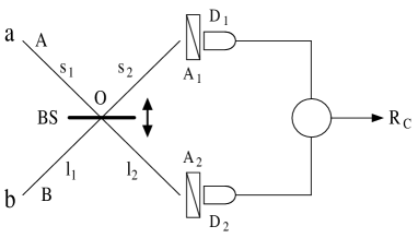
FIG. 5.: Schematic of the two-photon interferometer with polarization considered

In this theoretical scheme of two-photon interference experiment, a photon pair state with entanglement with polarization degrees of freedom can be written as

$$\left|\Psi\right\rangle = \int_{0}^{\infty}d\omega d\widetilde{\omega}f\left(\omega,\widetilde{\omega}\right)\times$$ (18)

$$\frac{1}{\sqrt{2}}\left[a_{AH}^{+}\left(\omega\right)a_{BV}^{+}\left(\widetilde{\omega}\right)-a_{AV}^{+}\left(\omega\right)a_{BH}^{+}\left(\widetilde{\omega}\right)\right]\left|0\right\rangle\text{.}$$

The photons arrive detector $D_{1}$ and $D_{2}$ after mixed by the beam splitter $BS$. Here $a_{AH}^{+}\left(\omega\right)$ is the creation operator of photon of frequency $\omega$, the wave vector is along direction $Oa$ (in optical path mode $A$) with horizontal polarization (along direction $\widehat{e}_{H}$). The notations $a_{BV}^{+}\left(\widetilde{\omega}\right)$, $a_{AV}^{+}\left(\omega\right)$ and $a_{BH}^{+}\left(\widetilde{\omega}\right)$ are defined similarly as $a_{AH}^{+}\left(\omega\right).$ Two polarization analyzers $A_{1}$ and $A_{2}$ along the directions $\widehat{A}_{1}$ and $\widehat{A}_{2}$ are put in front of the detectors.

It is easy to see that the rate $R_{c}$ of coincident detection is proportional to the time integral of the square of effective wave function $\psi$’s mode, i.e.

$\displaystyle R_{c}\propto\int dt_{1}dt_{2}\left|\psi\left(t_{1},t_{2}\right)\right|^{2}$

where

$$\psi\left(t_{1},t_{2}\right)=\left\langle 0\right|E_{1}^{+}\left(t_{1}\right)E_{2}^{+}\left(t_{2}\right)\left|\Psi\right\rangle\text{.}$$ (19)

Here $E_{i}^{+}\left(t_{i}\right)=\widehat{A}_{i}\cdot\overrightarrow{E_{i}^{+}}\left(t_{i}\right)$,and$\overrightarrow{\text{ }E_{i}^{+}}\left(t_{i}\right)=\widehat{e}_{H}$ $E_{H}^{+}\left(t_{i}\right)+\widehat{e}_{V}$ $E_{V}^{+}\left(t_{i}\right)$( $i=1,2)$ are the positive frequency parts of light field operator at the position of the detector. Considering the transforming character of beam splitter, we have

$$\overrightarrow{E_{1}^{+}}(t_{1}) = \frac{1}{\sqrt{2}}[i\overrightarrow{E_{a}^{+}}(\tau_{1})+\overrightarrow{E_{b}^{+}}(\tau_{1}^{\prime})]$$ (20)

$$\overrightarrow{E_{2}^{+}}(t_{2}) = \frac{1}{\sqrt{2}}[\overrightarrow{E_{a}^{+}}(\tau_{2}^{\prime})+i\overrightarrow{E_{b}^{+}}(\tau_{2})]\text{.}$$ (21)

Here $\tau_{1}$, $\tau_{1}^{\prime}$, $\tau_{2}$, $\tau_{2}^{\prime}$ are just defined as in section 2 and $\overrightarrow{E_{a}^{+}}_{\left(b\right)}=\widehat{e}_{H}$ $E_{a\left(b\right)H}^{+}+\widehat{e}_{V}$ $E_{a\left(b\right)V}^{+}$ are the positive frequence part of the light field operator at point $a$ and $b$ and $E_{a\left(b\right)H\left(V\right)}^{+}\left(t\right)=\int d\omega a_{A\left(B\right)H\left(V\right)}\exp\left[-i\omega t\right]$. The spectral density function $g\left(\omega\right)$ is neglected here without loss of generity.

Submitting 20 to 19, we can get the explicit expression  for effective wave function $\psi$ of the light field’s $:$

$$\psi = \frac{1}{2\sqrt{2}}\left[\widehat{A}_{1}\cdot\widehat{e}_{V}\times\widehat{A}_{2}\cdot\widehat{e}_{H}-\widehat{A}_{1}\cdot\widehat{e}_{H}\times\widehat{A}_{2}\cdot\widehat{e}_{V}\right]\times$$ (23)

$$\int d\omega d\widetilde{\omega}f\times\left[e^{-i\left(\widetilde{\omega}\tau_{1}^{\prime}+\omega\tau_{2}^{\prime}\right)}+e^{-i\left[\omega\tau_{1}^{\prime}+\widetilde{\omega}\tau_{2}^{\prime}+\left(\omega-\widetilde{\omega}\right)\frac{D}{c}\right]}\right]$$

where $D=l_{1}-s_{1}=c\left(\tau_{1}-\tau_{1}^{\prime}\right)$ $=c\left(\tau_{2}^{\prime}-\tau_{2}\right)$ is the optical path difference disscussed before. Then $R_{c}$ can be written as

$$R_{c}=\xi\left(\widehat{A}_{1},\widehat{A}_{2}\right)\times\eta\left(D\right)$$ (24)

where

$$\xi\left(\widehat{A}_{1},\widehat{A}_{2}\right)=\frac{1}{8}\left|\widehat{A}_{1}\cdot\widehat{e}_{V}\times\widehat{A}_{2}\cdot\widehat{e}_{H}-\widehat{A}_{1}\cdot\widehat{e}_{H}\times\widehat{A}_{2}\cdot\widehat{e}_{V}\right|^{2}$$ (25)

is dependent of the direction of polarization analyser and

$$\eta\left(D\right) = \int d\tau_{1}^{\prime}d\tau_{2}^{\prime}|\int d\omega d\widetilde{\omega}f\times$$ (27)

$$\left[e^{-i\left(\widetilde{\omega}\tau_{1}^{\prime}+\omega\tau_{2}^{\prime}\right)}+e^{-i\left[\omega\tau_{1}^{\prime}+\widetilde{\omega}\tau_{2}^{\prime}+\left(\omega-\widetilde{\omega}\right)\frac{D}{c}\right]}\right]|^{2}$$

varies as the optical path difference $D$ is changed.

It is easy to prove that, when the frequency distribution function $f$ is symetric, i.e. $f\left(\omega,\widetilde{\omega}\right)=f\left(\omega,\widetilde{\omega}\right),$ we have $\frac{d\eta}{dD}\mid_{D=0}$and

$$\frac{d^{2}\eta}{dD^{2}}\mid_{D=0}\propto-\int d\omega d\widetilde{\omega}\left|f\right|^{2}\left(\omega-\widetilde{\omega}\right)^{2}<0.$$ (28)

So we know that in this case $R_{c}$ has its maximal value when $D=0$. This is differenct to the case in which the photon polarization is not considered and $R_{c}$ has its minimal value when $D=0$. In fact, this difference is due to the $-1$ factor in light field’s initial state 18 i.e. if the initial state is

$$\int_{0}^{\infty}d\omega d\widetilde{\omega}f\times\frac{1}{\sqrt{2}}\left[a_{AH}^{+}\left(\omega\right)a_{BV}^{+}\left(\widetilde{\omega}\right)+a_{AV}^{+}\left(\omega\right)a_{BH}^{+}\left(\widetilde{\omega}\right)\right]\left|0\right\rangle,$$ (29)

$R_{c}$ will also has its minimal value when $D=0$.

It is notable that when the photon’s polarization is considered, $f\left(\omega,\widetilde{\omega}\right)=f\left(\omega,\widetilde{\omega}\right)$ is only the sufficient condition of that $R_{c}$ has its maximal value (or minimal value) when $D=0$ but not the necessary condition. In fact, it is difficult to obtain its necessary condition.

V Concluding remarks

To summarize, we have theoretically investigated the two photon interference phenomenon for a general situation with an arbitrary two photon state and given the necessary-sufficient condition for the destructive interference of coincidence counting in terms of the symmetric pairing of photons in the light pulses,i.e.,$G(\omega,\tilde{\omega})=0$. This implies that, even in the separable case $f(\omega,\tilde{\omega})=f_{1}(\omega)f_{2}(\tilde{\omega})$, if $f_{1}=f_{2},$a curve of ”dip” can still be observed in the rate of two photon coincidence. Our investigation predicts the destructive interference phenomenon to occur even for certain cases with separable input two photon state. However, this does not imply ”the interference between two independent photons” since the essence leading to destructive interference is that the required two photon state consists of the inseparable symmetric component$|S(\omega,\tilde{\omega}\rangle.$ Since for the the symmetric distribution function all components of the light field state have the entangled forms $|S(\omega,\tilde{\omega}\rangle$,we understand the ”dip” in the destructive coincidence curve according to the free induction decay mechanism from the dispersion of the two-photon frequency ($\omega,\tilde{\omega}$). In fact, though each component contributes $R_{c}$ with an oscillating term with respect to $D$, in the integral of variables $\tilde{\omega}$ and $\omega$ with Gaussian type distribution $f$ , these oscillating terms cancel one another and thus lead to a (anti-) Gaussian decaying factor. We also considered the effect of photon’s polarization. We found that,when the effective wave function is symetric i.e. $f\left(\omega,\tilde{\omega}\right)=f\left(\tilde{\omega},\omega\right)$, the coincidence counting rate may have its maximal or minimal value when the path difference is zero.

Acknowledgement: The authors thank Jian-wei Pan for his useful discussions. This work is supported by the NSF of China ( CNSF grant No.90203018) and the Knowledged Innovation Program(KIP) of the Chinese Academy of Science. It is also founded by the National Fundamental Research Program of China with No 001GB309310.

REFERENCES

• [1] Electronic address: suncp@itp.ac.cn
• [2] Internet www site: http:// www.itp.ac.cn/~suncp
• [3] A. Einstein, B. Podolsky, and N. Rosen, Phys. Rev. 47, 77-78(1935).
• [4] See, e.g., W.H. Louisell, A. Yariv, and A.E. Siegmann, Phys. Rev. 124 , 1646 (1961); D.N. Klyshko, Photons and Nonlinear Optics (Gordon and Breach Science, New York, 1988); T.G. Giallorentzi and C.L. Tang, Phys. Rev. 166, 255 (1968).
• [5] J. S. Bell, Physics 1, 195. (1964).
• [6] C.O. Alley and Y.H. Shih Proceedings of the Second International Symposium on Foundations of Quantum Mechanics in the Light of New Technology M. Namiki (Ed.) (1986).
• [7] Y.H. Shih and C.O. Alley, Phys. Rev. Lett. 61 2921 (1988).
• [8] Z.Y. Ou and L. Mandel, Phys. Rev. Lett. 61 50 (1988).
• [9] The Physics of Quantum Information D. Bouwmeeste, A. Ekert and A. Zeilinger (Ed.) (Springe, Berlin, 2000).
• [10] K.A.M. Dirac, Principle of Quantum Mechanics, 4ed. (Oxford, Oxford 1958).
• [11] C.K. Hong, Z.Y. Ou and L. Mandel, Phys. Rev. Lett. 59, 2044 (1987).
• [12] P.G. Kwiat, A.M. Steinberg and R.Y. Chiao, Phys. Rev. A. 45, 7729 (1992).
• [13] S. P. Walborn, A. N. de Oliveira, S. Padua and C. H. Monken quan-ph/0212017
• [14] T.B. Pittman, D.V. Strekalov, A. Migdall, M.H. Rubin, A.V.Sergienko and Y.H. Shih, Phys. Rev. Lett. 77, 1917 (1996).
• [15] D.V. Strekalov, T.B. Pittman and Y.H. Shih, Phys. Rev. A. 57, 567 (1998).
• [16] Y.H. Shih, Advances in Atomic, Molecular and Optical Physics. 41 1 (1999)
• [17] E.L.Hahn,Phys. Rev. 77, 297(1950); R. G. Brewer, R.L. Shoemaker,Phys. Rev. A 6, 2001(1972); also see L.Mandel, E.Wolf, Optical Coherence and Quantum Optics,Cambridge Univ.Press, 1995,p.805.
• [18] R. J. Glauber, Phys. Rev. 130, 2529(1963).
• [19] R. J. Glauber, Phys. Rev. 131, 2766(1963).
• [20] D.L.Zhou, P.Zhang, C.P.Sun, Phys. Rev.A 66,012112(2002)
• [21] W. P. Grice and I. A. Walmsley, Phys. Rev. A 56, 1627(1997)
• [22] Timothy E. Keller and Morton H. Rubin, Phys. Rev. A 56, 1534(1997)
• [23] W. P. Grice, A. B. URen and I. A. Walmsley, Phys. Rev. A 64, 063815(2001)
• [24] V. Giovannetti, L. Maccone, J. H. Shapiro, and F. N. C. Wong, Phys. Rev. Lett 88, 183602(2002)
• [25] J. Bylander, I. R. Philip and I. Abram, Eur. Phys. J. D 02036-6(2002)
• [26] H. de Riedmatten, I. Marcikic, W. Tittel, H. Zbinden and N. Gisin, quan-ph/0208174