Bohmian Histories and Decoherent Histories

Abstract

The predictions of the Bohmian and the decoherent (or consistent) histories formulations of the quantum mechanics of a closed system are compared for histories — sequences of alternatives at a series of times. For certain kinds of histories, Bohmian mechanics and decoherent histories may both be formulated in the same mathematical framework within which they can be compared. In that framework, Bohmian mechanics and decoherent histories represent a given history by different operators. Their predictions for the probabilities of histories of a closed system therefore generally differ. However, in an idealized model of measurement, the predictions of Bohmian mechanics and decoherent histories coincide for the probabilities of records of measurement outcomes. The formulations are thus difficult to distinguish experimentally. They may differ in their accounts of the past history of the universe in quantum cosmology.

I Introduction

Bohmian mechanics (e.g. BH93 ) and decoherent (or consistent) histories quantum mechanics (e.g. Gri84 ; Omn94 ; GH90a ) are formulations of quantum mechanics that share some common objectives. Both are formulations of quantum mechanics for a closed system such as the universe. Both are formulations of quantum mechanics that do not posit a privileged, fundamental role for measurements or the observers that make them. The question of the relationship between these two formulations has been addressed in several different places BH93 ; Ken96 ; Gri99 ; HM00 . This paper compares the predictions of the two formulations for histories — time sequences of alternatives for the closed system. We make the following points:

• For certain classes of histories, Bohmian mechanics and decoherent histories (for short) may both be formulated within the same mathematical framework of a Hilbert space of states, operators representing alternatives, and unitary evolution. Within this framework they may be compared.

• Bohmian mechanics and decoherent histories generally represent the same history by different operators. Their predictions for the probabilities of histories will therefore generally differ.

• In an idealized model of measurement, Bohmian mechanics and decoherent histories predict the same probabilities for records of the outcomes of measurements. This makes it difficult to distinguish the formulations experimentally.

Not surprisingly, there is overlap of our comparison of Bohmian mechanics and decoherent histories with others especially that of Griffiths Gri99 . However, we do not aim in this paper to present arguments for or against either formulation of the quantum mechanics of closed, non-relativistic systems. We intend to merely point out some differences between them.

After a necessary review of the two formulations in Section II, we establish the above three facts in Sections III–V. We conclude with some brief discussion of possible differences between the descriptions given by Bohmian mechanics and decoherent histories of the past in cosmology.

II Bohmian Mechanics and Decoherent Histories

II.1 A Model Closed System

To establish the facts listed in the Introduction, it is sufficient to use the illustrative (but unrealistic) model of a universe of $N$ non-relativistic particles in a box. The dynamics of the positions $\vec{x}_{1},\cdots,\vec{x}_{N}$ is governed by a Hamiltonian assumed to be of the form

$$H=\sum^{N}_{i=1}\ \frac{\vec{p}^{\,2}_{i}}{2m_{i}}+V(\vec{x}_{1},\cdots,\vec{x}_{n})\ .$$ (1)

In addition to the Hamiltonian $H$, we assume that the initial quantum state of the closed system $|\Psi\rangle$ is given at time $t=t_{0}=0$. Its configuration space representative is the initial wave function

$$\Psi\left(\vec{x}_{i},0\right)\equiv\left\langle\vec{x}_{1},\cdots\vec{x}_{n}|\Psi\right\rangle\ .$$ (2)

The most general objective of a quantum mechanical theory of a closed system is the prediction of the probabilities of the individual members of a set of alternative, coarse-grained, time histories of the system. For example, if the box contained the solar system, probabilities of different orbits of the earth around the sun might be of interest. These orbits are histories of the position of the center of mass of the earth at a sequence of times. A coarse-grained history might be specified by giving a sequence of ranges $\Delta_{1},\cdots,\Delta_{n}$ for the center of mass position of the earth at a series of times $t_{1},\cdots,t_{n}$. The history is coarse grained because the position of every particle in the box is not specified, the center of mass position is not specified to arbitrary accuracy, and not at all possible times. Bohmian mechanics is usually formulated in terms of histories of position, so it will be convenient to restrict the further discussion to histories of this type. Specifically, we consider histories specified by giving exhaustive sets of exclusive regions $\{\Delta^{k}_{\alpha_{k}}\}$, $\alpha_{k}=1,2,\cdots$, of the configuration space of the $\vec{x}_{i}$’s at a series of times $t_{k}$, $k=1,\cdots,n$. A history is thus specified by a series of regions $(\alpha_{n},\cdots,\alpha_{1})$ which we denote by $\alpha$ for short.

II.2 Decoherent Histories Quantum Mechanics

We now briefly review how (and when) decoherent histories quantum mechanics assigns probabilities to a history $\alpha\equiv(\alpha_{n},\cdots,\alpha_{1})$ of ranges of position at a series of times $t_{1},\cdots,t_{n}$. For more details in the present notation see, e.g. GH90a ; Har93a .

The alternative regions of configuration space $\{\Delta^{k}_{\alpha_{k}}\}$ correspond to an exhaustive set of exclusive (Schrödinger picture) projection operators $\{P^{k}_{\alpha_{k}}\}$ that project onto these regions. Because the regions are exhaustive and exclusive these projection operators satisfy (for each $k$)

$$P^{k}_{\alpha_{k}}P^{k}_{\alpha^{\prime}_{k}}=\delta_{\alpha_{k}\alpha^{\prime}_{k}}P^{k}_{\alpha_{k}}\quad,\quad\sum\nolimits_{\alpha_{k}}P^{k}_{\alpha_{k}}=I\ .$$ (3)

A history of alternatives $\alpha=(\alpha_{n},\cdots,\alpha_{1})$ at times $t_{1},\cdots,t_{n}$ is represented by the corresponding chain of projections interspersed with unitary evolution

$$C_{\alpha}\equiv P^{n}_{\alpha_{n}}U\left(t_{n},t_{n-1}\right)P^{n-1}_{\alpha_{n-1}}U\left(t_{n-1},t_{n-2}\right)\cdots P^{1}_{\alpha_{1}}U\left(t_{1},0\right)\ ,$$ (4)

where

$$U\left(t^{\prime\prime},t^{\prime}\right)=e^{-iH\left(t^{\prime\prime}-t^{\prime}\right)/\hbar}\ ,$$ (5)

and $t=t_{0}=0$ is the time of the initial condition.

The probabilities $p_{\alpha}$ of the individual histories in a set of alternative histories are given by

$$p^{(DH)}_{\alpha}=\left\|C_{\alpha}|\Psi\rangle\right\|^{2}\ .$$ (6)

However, decoherent histories quantum mechanics does not assign probabilities to every set of histories that may be described. The numbers (6) may be inconsistent with the rule that the probability of a coarser-grained set of alternatives should be the sum of probabilities of its members. Rather, probabilities are assigned only to sets of alternative histories that are consistent Gri84 , for example by satisfying the decoherence condition

$$\langle\Psi|C^{\dagger}_{\alpha^{\prime}}C_{\alpha}|\Psi\rangle\approx 0\quad{\rm for}\ \alpha^{\prime}\not=\alpha\ .$$ (7)

We stress that “decoherence”, “decoherent” , etc. as used in this paper refer to the absence of interference between the histories in an exhaustive set of alternative histories as specified quantitatively by (7). We do not mean a process in which a reduced density matrix becomes approximately diagonal which is another common usage of these terms.

II.3 Bohmian Mechanics

In Bohmian mechanics, the trajectories of the particles in the box obey two deterministic equations. The first is the Schrödinger equation for $\Psi$.

$$i\hbar\ \frac{\partial\Psi}{\partial t}=H\Psi\ .$$ (8a)

Then, writing $$\Psi=R\exp(iS) R S \vec{x}_{i}(t)$$ with and real, the second is the deterministic equation for the

$$m_{i}\ \frac{d\vec{x}_{i}}{dt}=\vec{\nabla}_{\vec{x}_{i}}S\left(\vec{x}_{1},\cdots,\vec{x}_{N}\right)\ ,$$ (8b)

The initial wave function (2) is the initial condition for (8a). The theory becomes a statistical theory with the assumption that the initial values of the $\vec{x}_{i}$ are distributed according to the probability density on configuration space

$$\wp\left(\vec{x}_{1},\cdots,\vec{x}_{N}\,,0\right)=\left|\Psi\left(\vec{x}_{1},\cdots,\vec{x}_{N},0\right)\right|^{2}\ .$$ (9)

Once this initial probability distribution is fixed, the probability of any later alternatives is fixed by the deterministic equations (8b).

A coarse-grained Bohmian history $\alpha\equiv(\alpha_{n},\cdots,\alpha_{1})$ defined by a sequence of ranges $\{\Delta^{k}_{\alpha_{k}}\}$ of the $\vec{x}_{i}$ at a series of times consists of the set of Bohmian trajectories $\vec{x}_{i}(t)$ that cross those ranges at the specified times.

III Bohmian and Decoherent Histories

III.1 Bohmian Histories

An individual Bohmian trajectory $\vec{x}_{i}(t)$ is fixed deterministically by equations (8b) once the initial condition $\vec{x}_{i}(0)$ and the initial value of $\Psi$ are given. The probability of a coarse-grained history $\alpha\equiv(\alpha_{n},\cdots,\alpha_{1})$ is therefore the probability of the region of initial $\vec{x}_{i}(0)$’s that lead to trajectories that pass through the regions $\Delta^{n}_{\alpha_{n}},\cdots,\Delta^{1}_{\alpha_{1}}$ at times $t_{1},\cdots,t_{n}$. We call this range of initial values $\Delta^{(BM)}_{\alpha_{1}\cdots\alpha_{n}}$ or $\Delta^{(BM)}_{\alpha}$ for short. Denote by $B_{\alpha}$ the projection on this range of $\vec{x}_{i}(0)$’s corresponding to the history $\alpha$. From (9) the probability $p^{(BM)}_{\alpha}$ predicted by Bohmian mechanics for this history is

$$p^{(BM)}_{\alpha}=\|B_{\alpha}|\Psi\rangle\|^{2}\ .$$ (10)

The operator $B_{\alpha}$ is not determined by the ranges $\Delta^{n}_{\alpha_{n}},\cdots,\Delta^{1}_{\alpha_{1}}$ alone but also depends on the initial state $\Psi$. That is because the evolution of $\Psi$ through (8b) is needed to determine whether the trajectories pass through the regions $\Delta^{n}_{\alpha_{n}},\cdots,\Delta^{1}_{\alpha_{1}}$.

III.2 Different Probabilities for the Same History

The Bohmian formula (10) is an expression for the probabilities of a set of histories that is in the same mathematical framework as (6) for decoherent histories. It is thus possible to compare the two formulations.

Figure 1: The motion of wave packets in the BESSW example. Two wave packets initially localized (at $t=0$) within the circles at left have equal and opposite $y$-components of their expected momentum $\vec{p}$. The wave packets evolve through the shaded regions indicated to the positions shown at $t=t_{7}$. At intermediate times $t_{1},\cdots t_{6}$, they are centered in one or the other of the squares.

We first note that decoherence in the sense of the absence of interference between multi-time histories [cf (7)] is automatic for sets of Bohmian histories. The $B_{\alpha}$ are orthogonal projections onto disjoint regions of the initial $\vec{x}_{i}(0)$ and satisfy $B_{\alpha}B_{\alpha^{\prime}}=\delta_{\alpha\alpha^{\prime}}B_{\alpha}$ [cf. (3)]. Thus,

$$\langle\Psi\left|B^{\dagger}_{\alpha}B_{\alpha^{\prime}}\right|\Psi\rangle\equiv 0\quad,\quad\alpha\not=\alpha^{\prime}\ .$$ (11)

Consistency of Bohmian probabilities is automatic.

This is the first of the differences between the Bohmian mechanics and the decoherent histories formulations of quantum theory: Bohmian mechanics assigns probabilities to sets of histories of position that do not decohere. Bohmian mechanics therefore potentially assigns probabilities to more sets of histories of position than decoherent histories. However, when histories of alternatives other than position are considered, the situation is the other way around. The decoherent histories formulation assigns probabilities to histories of alternatives defined by ranges of operators other than position which are not represented, at least not fundamentally, in Bohmian mechanics.

A comparison of the probability expressions (10) and (6) reveals a second and more important difference. In general, Bohmian mechanics and decoherent histories predict different probabilities for the same history. That is because the operator $B_{\alpha}$ corresponding to a history in Bohmian mechanics is a projection while the operator $C_{\alpha}$ is decoherent histories is generally not. We shall give explicit examples below.

We should perhaps stress that we are not referring here to histories of measurements of position carried out by some external system. We are rather considering both Bohmian mechanics and decoherent histories as quantum theories of a closed system containing measurement apparatus if any. The special situation with histories of measured alternatives will be discussed in Section IV.

The one general case when the probabilities coincide are when the set of histories is so coarse grained that it consists of alternatives $\{P_{\alpha}\}$ at a single moment of time $t_{1}$

$$C_{\alpha}=P_{\alpha}U\left(t_{1},0\right)\ .$$ (12)

Probability is conserved along Bohmian trajectories. Specifically it follows from (8b) that

$$\frac{\partial\wp}{\partial t}+\sum^{N}_{i=1}\vec{\nabla}_{\vec{x}_{i}}\cdot\left(\wp\ \frac{\nabla_{\vec{x}_{i}}S}{m_{i}}\right)=0$$ (13)

where $\wp=\left|\Psi\left(\vec{x}_{i},t\right)\right|^{2}$. Therefore, since $B_{\alpha}$ are projections on the range of positions at $t=0$ of trajectories that pass through the regions defined by $P_{\alpha}$ at time $t$,

$$\left\|P_{\alpha}U\left(t_{1},0\right)|\Psi\rangle\right\|^{2}=\left\|B_{\alpha}|\Psi\rangle\right\|^{2}\ ,$$ (14)

and

$$p_{\alpha}^{(DH)}=p^{(BM)}_{\alpha}\quad,\quad({\rm for\ single\ time\ histories)}\ .$$ (15)

The time $t_{1}$ is arbitrary. Probabilities of histories restricted to a single time coincide for all values of that time. But most physically interesting histories are described by alternatives at more than one time. For example, predictions of the orbit of the Mars around the Sun involve the conditional probabilities for future positions of the Mars given some observations of its position in the past. Those are constructed from the probabilities of histories of the location of Mars at multiple times in the past and future. Indeed, in the context of quantum cosmology, very few useful predictions can be expected from alternatives at a single time conditioned only by the initial state of the universe $|\Psi\rangle$ (see, e.g. Har03a ).

III.3 An Example

Several situations that have been widely discussed in Bohmian mechanics provide examples where the probabilities predicted by Bohmian mechanics differ significantly from those of decoherent histories. Bel80 ; Engsum ; DFGZ93 ; DHS93 ; AV96 ; HCM00 ; Gri99 . We call these BESSW examples. A simple case is illustrated in Figure 1.

A single free particle moves in a two-dimensional plane. The plane is divided into square regions that will be used to describe coarse-grained histories of the particle’s position. (The squares are the $\{\Delta^{k}_{\alpha_{k}}\}$ with the same set of ranges for each $k$.) The initial wave function is a superposition of two wave packets $G(x,y,0)$ and $G(x,-y,0)$, viz.,

$$\Psi(x,y,0)=\frac{1}{\sqrt{2}}\ \left[G(x,y,0)+G(x,-y,0)\right]\ .$$ (16)

The wave packet $G(x,y,0)$ is assumed to be localized well within the dimensions of one initial square as shown, and to have a momentum $\vec{p}$ defined within the limits of the uncertainty principle with a negative component of $p_{y}$. The wave packet $G(x,-y,0)$ is initially located symmetrically about the $y$ axis and has an equal magnitude but positive component of $p_{y}$. Evolved by the Schrödinger equation over a time interval short compared to that for significant spreading, the wave packets will move through the shaded regions shown in Figure 1.

To define a set of alternative histories, choose a sequence of equally spaced times $t_{1},t_{2},\cdots,t_{7}$ when each wave packet is within one of the squares encompassing its path. A set of all possible coarse-grained histories is then the set of all possible sequences of squares at these times. We now calculate the probabilities assigned by Bohmian mechanics and decoherent histories to this set of alternative coarse-grained histories. Our analysis does not differ substantially from that presented by Griffiths Gri99 for the same class of examples.

The probabilities predicted by decoherent histories are given by (6) and (4). The action of the operator $C_{\alpha}$ can be described as successive projections (or “reductions”) on the sequence of squares defining the history interspersed with unitary evolution. The unitary evolution moves the wave packet as described above. Since the wave packets are within one square or another at the times $t_{1},\cdots,t_{7}$, the projections have almost no effect on them. Thus, for the history $\alpha=\alpha_{+}$ corresponding to the sequence of squares that track the wave packet starting at upper left

$$\langle x,y|C_{\alpha_{+}}|\Psi\rangle\approx\frac{1}{\sqrt{2}}\ G\left(x,y,t_{7}\right)\ .$$ (17a)

Similarly for the $$\alpha=\alpha_{-}$$ history corresponding to the squares that track the wave packet starting at lower left

$$\langle x,y|C_{\alpha_{-}}|\Psi\rangle\approx\frac{1}{\sqrt{2}}\ G\left(x,-y,t_{7}\right)\ .$$ (17b)

For all other sequences of squares

$$\langle x,y\left|C_{\alpha}\right|\Psi\rangle\approx 0\ ,\quad\alpha\not=\alpha_{\pm}\ .$$ (17c)

These facts imply that the set of histories is approximately decoherent because the only potentially non-zero, off-diagonal inner product is

$$\langle\Psi\left|C^{\dagger}_{\alpha_{+}}C_{\alpha_{-}}\right|\Psi\rangle\approx 0\ .$$ (18)

This is negligible because there is almost no overlap between the two wave packets at $t_{7}$. The only non-vanishing probabilities are for the sequences $\alpha_{+}$ and $\alpha_{-}$ with

$$p^{(DH)}_{\alpha_{+}}=p^{(DH)}_{\alpha_{-}}\approx\frac{1}{2}\ .$$ (19)

These two histories are illustrated in Figure 2.

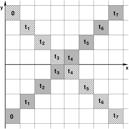
Figure 2: Coarse-grained histories with high probability in the BESSW example according to decoherent histories quantum mechanics. Coarse-grained histories are defined by the grid of square regions at a sequence of times $t_{1},\cdots,t_{7}$ adjusted so that the wave packets of Fig. 1 are centered in one square at each time. The possible coarse-grained histories are the sequence of any seven squares at the series of times. The two sequences of squares which have any significant probability according to decoherent histories quantum mechanics are shown, distinguished by different shadings.

We now turn to the predictions of Bohmian mechanics for the same set of histories. Because $\Psi(x,y,0)$ is symmetric about the $x$-axis, and because the Hamiltonian commutes with this symmetry, it holds for all times when $\Psi(x,y,0)$ is evolved by the Schrödinger equation (8a)

$$\Psi(x,y,t)=\Psi(x,-y,t)\ .$$ (20)

Then from (8b)

$$\left(\frac{dy}{dt}\right)_{x=0}=0$$ (21)

for all times. No Bohmian trajectory crosses the $x$-axis. In particular,

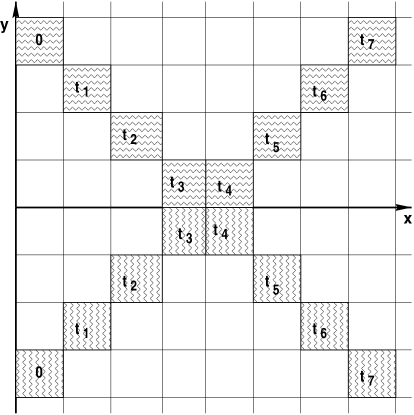
Figure 3: Coarse-grained histories with high probability in the BESSW example according to Bohmian mechanics. The coarse-grained histories are the same as those in Fig. 2 (q.v.). The two sequences of squares with any significant probability are shown, distinguished by different shadings. They are different from those predicted by decoherent histories.

$$p^{(BM)}_{\alpha_{+}}=p^{(BM)}_{\alpha_{-}}\approx 0\ .$$ (22)

The two histories for which Bohmian mechanics predicts non-negligible probabilities are sketched in Figure 3. However, only a comparison of (19) and (22) is necessary to demonstrate conclusively that decoherent histories and Bohmian mechanics generally predict different probabilities for the same set of alternative coarse-grained histories of a closed system.

The reason for the difference is also illustrated by this example. We mentioned that the action of the $C_{\alpha}$ could be thought of as unitary evolution interspersed with reduction. But in Bohmian mechanics, the wave function is never reduced. It evolves on forever by the Schrödinger equation undisturbed by any “second law of evolution”.

An important point illustrated by the BESSW example is that Bohmian trajectories while always deterministic are not necessarily classically deterministic. Quantum effects can be important for Bohmian trajectories even in situations where (as here) wave packets move approximately classically.

III.4 Another Viewpoint

Mathematically, the different predictions of Bohmian mechanics and decoherent histories arise because the same history $\alpha$ is represented by different operators — $B_{\alpha}$ and $C_{\alpha}$ respectively. However, from the decoherent histories viewpoint, the $B_{\alpha}$ describe a set of single time histories of various ranges of position $\Delta^{(BM)}_{\alpha}$ at $t=0$. (Recall the definition of $B_{\alpha}$ in Section III.A.) That is, the operator $B_{\alpha}$ describes a history in the decoherent histories formulation of quantum mechanics — not a sequence of alternatives at a series of times, but a certain range of positions at one time. Mathematically, therefore Bohmian mechanics is a restriction of decoherent histories quantum mechanics to histories represented by operators of a particularly simple type. Within decoherent histories quantum mechanics, the range $\Delta^{(BM)}_{\alpha}$ could be described as “the range of initial positions which, if evolved by the equations of Bohmian mechanics, would lead to trajectories passing through the $\{\Delta^{k}_{\alpha_{k}}\}$ at times $t_{k}$”. Bohmian mechanics would thus be employed merely as a tool for describing certain single time histories in decoherent histories quantum mechanics. However, to adopt this position would be tendentious. We will take the alternative view that Bohmian mechanics is not merely a different way of describing operators, but is a different way of interpreting them. In particular we will take the view that Bohmian mechanics and decoherent histories represent the same history by different operators and therefore may be different predictions for their probabilities. In the next section we discuss whether these can be observed.

IV Measurements

Are the different predictions of Bohmian mechanics and decoherent histories testable by experiments? That depends on whether the two formulations predict different probabilities for the outcomes of measurements. In this section we analyze this question employing idealizations common in many measurement models. (See, e.g. Har91a .)

Both Bohmian mechanics and decoherent histories are formulations of quantum mechanics for a closed system that do not posit a fundamental role for measurements or observers. Measurements and observation can, of course, be described in a closed system that contains both observer and observed, both measured subsystem and measurement apparatus. With suitable idealizations, the usual results of the approximate quantum mechanics of measured subsystems (Copenhagen quantum mechanics) are recovered to an excellent approximation Har91a .

Various general characterizations of measurement have been proposed — an “irreducible act of amplification”, “correlation of a ‘microscopic’ variable with a ‘macroscopic’ variable”, etc. It has proved difficult to make such ideas precise (e.g. what is “macroscopic”?), but a precise and general characterization is not needed in a quantum mechanics of a closed system. One characteristic which seems generally agreed upon is that the results of a measurement must be recorded — at least for a time. Histories of measurements whose outcomes are recorded can be modeled as follows in a closed system containing both measurement apparatus and measured subsystem.

For simplicity consider a single apparatus which carries out a series of measurements on another subsystem over a series of times. The apparatus records the sequence of outcomes for examination at some time $t_{R}$ after all the measurements are completed. Let $\{R_{\alpha}\}$ be set of orthogonal projection operators describing the alternative values of these records at $t_{R}$. To preserve the contact with Bohmian mechanics we shall assume that the $R$’s are projections onto ranges of the $x^{\prime}s$, as is plausibly the case for records of many realistic measurement situations.

Bohmian mechanics and decoherent histories will agree on the predictions of probabilities for the alternative outcomes of the measurements registered in these records. That is because the $\{R_{\alpha}\}$ represent alternatives at a single time whose probabilities generally agree as discussed in the last section [cf (15)]. Thus, if the result of every experiment can be summarized in records that are coarse-grained alternatives of the positions $\vec{x}_{i}$ at a single time, there seems little prospect that experiment can distinguish Bohmian mechanics from decoherent histories.

However, even if there is agreement on the probabilities of the records there can be disagreement on what they record, or indeed whether they are records at all, in situations where Bohmian mechanics and decoherent histories disagree on the probabilities of histories. To understand this let us first review more precisely what it means for a set of projection operators $\{R_{\alpha}\}$ to be a record of a history beginning with the case of decoherent histories.

Let $C_{\alpha_{n}\cdots\alpha_{1}}$ be the operator representing a history of coarse-grained alternatives that have been measured, and let $R^{(C)}_{\beta_{n}\cdots\beta_{1}}$ denote the orthogonal projections onto the various possible values of a record of the measurements. (The superscript “$C$” stands for “records of the $C$’s” — not “consistent”.) In an ideal measurement situation, the records at a later time $t_{R}$ are exactly correlated with the history of measured alternatives, viz.

$$R^{(C)}_{\beta_{n}\cdots\beta_{1}}e^{-iH(t_{R}-t_{n})/\hbar}C_{\alpha_{n}\cdots\alpha_{1}}|\Psi\rangle\propto\delta_{\beta_{n}\alpha_{n}}\cdots\delta_{\beta_{1}\alpha_{1}}\ ,$$ (23)

a relation we abbreviate by

$$R^{(C)}_{\beta}e^{-iH(t_{R}-t_{n})/\hbar}C_{\alpha}|\Psi\rangle=\delta_{\beta\alpha}R^{(C)}_{\alpha}e^{-iH(t_{R}-t_{n})/\hbar}C_{\alpha}|\Psi\rangle\ .$$ (24)

The relations obtained by summing (24) over $\alpha$, or alternatively over $\beta$, and using $\Sigma_{\beta}R_{\beta}=I$, $\Sigma_{\alpha}C_{\alpha}=U(t,t_{0})$ show that

$$R^{(C)}_{\beta}e^{-iH(t_{R}-t_{0})/\hbar}|\Psi\rangle=e^{-iH(t_{R}-t_{n})/\hbar}C_{\alpha}|\Psi\rangle\ .$$ (25)

The probabilities of the records of measurement outcomes are therefore the same as the probabilities of the histories

$$p^{(DH)}_{\alpha}\equiv\left\|C_{\alpha}|\Psi\rangle\right\|^{2}=\left\|R^{(C)}_{\alpha}e^{-iH(t_{R}-t_{0})/\hbar}|\Psi\rangle\right\|^{2}\ .$$ (26)

The situation in Bohmian mechanics is analogous with $C_{\alpha}$ replaced by $B_{\alpha}$, $R^{(C)}_{\alpha}$ by $R^{(B)}_{\alpha}$, $p^{(DH)}_{\alpha}$ by $p^{(BM)}_{\alpha}$, etc. The analogs of (24) and (26) are

$$R^{(B)}_{\beta}e^{-iH(t_{R}-t_{0})/\hbar}B_{\alpha}|\Psi\rangle=\delta_{\alpha\beta}R^{(B)}_{\alpha}e^{-iH(t_{R}-t_{0})/\hbar}B_{\alpha}|\Psi\rangle\ .$$ (27)

and

$$p^{(B)}_{\alpha}\equiv\left\|B_{\alpha}|\Psi\rangle\right\|^{2}=\left\|R^{(B)}_{\alpha}e^{-iH(t_{R}-t_{0})/\hbar}|\Psi\rangle\right\|^{2}\ .$$ (28)

However, when the predictions of Bohmian mechanics and decoherent histories differ, (24) and (26) cannot be both true with the same set of records $R^{(C)}_{\alpha}=R^{(B)}_{\alpha}\equiv R_{\alpha}$ because that would imply the equality of probabilities through (25) and (27). For instance, in the sequence of measurements described above, the records of outcomes $\{R_{\alpha}\}$ can correlated either with the histories $\{C_{\alpha}\}$ or the Bohmian trajectories $\{B_{\alpha}\}$ but not both if $p^{(DH)}_{\alpha}\neq p^{(BM)}_{\alpha}$ The situations disussed in Engsum where a detector localized in one region of space registers a particle whose Bohmian trajectory is elsewhere are examples. The devices that measure position are not recording the position of the Bohmian trajectory. Conversely, in these situations different apparatus with different records would be needed to measure the histories or the Bohmian trajectories.

V The Past in Quantum Cosmology

Probabilities for the records of measurement outcomes are not the only probabilities of interest in physics. For example, in cosmology, and in other areas of inquiry, the probabilities of past history are central to our understanding of the present.

Quantum mechanically, past history is a sequence of past events that is correlated with our present records with high probability. Why bother calculating these probabilities and using them to reconstruct the past? It’s over and done with. Reconstructing the past is useful because it simplifies the prediction of the future. (See, e.g. Har98b ). Take, for example, our understanding of the history of the very early universe from which we predict the present large scale distribution of the galaxies and the abundances of the elements in parts of the universe as yet unseen. We do not measure this early history. We infer with high probability from present observations. In principle, those same predictions could be made from a theory of the initial condition and the corpus of records of present instrumental observations, but it is much easier to first reconstruct the universe’s past history from these, and from that predict the future.

As the BESSW example makes clear, Bohmian mechanics and decoherent histories could differ significantly in their accounts of the past. That can be true even when approximate classical determinism holds in decoherent histories. Bohmian trajectories are not necessarily classical although they are always deterministic.

The BESSW example is very special. It is a simple model with one free particle and a very particular initial condition. It does not generalize naturally to many interacting particles moving in three-dimensions. Yet more realistic three-dimensional calculations with initial states that are in a superposition of wave packets whose centers follow classical orbits show similar non-classical behavior for Bohmian trajectories Erlerun .

The question of whether the Bohmian trajectories describing the realistic past of our universe behave classically or not is an interesting question for future investigation. As a starting point, however, it is worth noting that it is unlikely that the initial wave function of the universe assigns a definite position to each galaxy. To do so it would have to encode the complexity of the present large scale distribution of galaxies. Rather, a simple, discoverable, initial condition might be expected to be a superposition of all possible configurations of initial positions. Then the complexity of the present distribution of galaxies arose from chance accidents over the course of the universe’s history rather than deterministically from a complex initial condition. Contemporary theories of the initial condition, such as Hawking’s wave function of the universe HHaw85 , have this superposition character.

Suppose the Bohmian trajectories arising from a realistic wave function of the universe were to exhibit significant non-classical behavior in the epochs where the corresponding coarse-grained decoherent histories behaved classically with high probability. Bohmian mechanics and decoherent histories formulations of quantum mechanics would then agree on the record of every measurement outcome, but disagree on the fundamental description of the past. If so they might differ in their utility for cosmology.

- (1) D. Bohm and B.J. Hiley, The Undivided Universe, Routledge, London, (1993).
- (2) R.B. Griffiths, J. Stat. Phys., 36, 219, 1984.
- (3) R. Omnès, Interpretation of Quantum Mechanics, (Princeton University Press, Princeton, 1994).
- (4) M. Gell-Mann and J.B. Hartle, in Complexity, Entropy, and the Physics of Information, SFI Studies in the Sciences of Complexity, Vol. VIII, ed. by W. Zurek, Addison Wesley, Reading, MA (1990).
- (5) A.P.A. Kent, in Bohmian Mechanics and Quantum Theory: An Appraisal, ed. by J. Cushing, A. Fine and S. Goldstein, (Kluwer Academic Press, Dordrecht, 1996), pp. 343-352, quant-ph/9511032.
- (6) R.B. Griffiths, Phys.Lett., A261, 227 (1999); quant-ph/9902059.
- (7) B.J. Hiley and O.J.E. Maroney, quant-ph/0009056.
- (8) M. Gell-Mann and J.B. Hartle, Time Symmetry and Asymmetry in Quantum Mechanics and Quantum Cosmology in Physical Origins of Time Asymmetry, ed. by J. Halliwell, J. Perez-Mercader, and W. Zurek, Cambridge University Press, Cambridge (1994) pp. 311-345; gr-qc/9304023.
- (9) J.B. Hartle, Theories of Everything and Hawking’s Wave Function of the Universe, in The Future of Theoretical Physics and Cosmology, ed. by G.W. Gibbons, E.P.S. Shellard, and S.J. Rankin, Cambridge University Press, Cambridge, 2003, pp.38-50, gr-qc/0209104.
- (10) J.B. Hartle, in Directions in General Relativity, Volume 1: A Symposium and Collection of Essays in honor of Professor Charles W. Misner’s 60th Birthday, ed. by B.-L. Hu, M.P. Ryan, and C.V. Vishveshwara, Cambridge University Press, Cambridge (1993). gr-qc/9210006.
- (11) J.S. Bell, Intl. J. Quant. Chem, Quantum Chemistry Symposium 14, John Wiley, New York (1980), pp. 155–159 [Reprinted in J.S. Bell, Speakable and Unspeakable in Quantum Mechanics, Cambridge University Press, Cambridge (1987), p.111-116].
- (12) B.-G. Englert, M.W. Scully, G. Süssmann, and H. Walther, Z. Naturforsch, 47a, 1175 (1992); ibid., Z. Naturforsch, 48a, 1263 (1993).
- (13) D. Dürr, W. Fusseder, S. Goldstein, and N. Zanghi, Z. Naturforsch, 48a, 1261 (1993).
- (14) C. Dewdney, L. Hardy, and E.J. Squires, Phys. Lett. A184, 6 (1993).
- (15) Y. Aharonov and L. Vaidman, in Bohmian Mechanics and Quantum Theory: An Appraisal, ed. by J. Cushing, A. Fine and S. Goldstein, (Kluwer Academic Press, Dordrecht, 1996).
- (16) B.J. Hiley, R.E. Callaghan and O.J.E. Maroney, quant-ph/0010020.
- (17) J.B. Hartle, in Quantum Cosmology and Baby Universes: Proceedings of the 1989 Jerusalem Winter School for Theoretical Physics, ed. by S. Coleman, J.B. Hartle, T. Piran, and S. Weinberg, World Scientific, Singapore (1991), Section II.10, pp. 65-157.
- (18) J.B. Hartle, Physica Scripta, T76, 67–77 (1998); gr-qc/9712001.
- (19) T. Erler (unpublished).
- (20) J. Halliwell and S.W. Hawking, Phys. Rev. D 31, 1777, 1985.