Generalized Zero Range Potentials and Multi-Channel Electron-Molecule Scattering

Abstract

A multi-channel scattering problem is studied from a point of view of integral equations system. The system appears while natural one-particle wave function equation of the electron under action of a potential with non-intersecting ranges is considered. Spherical functions basis expansion of the potentials introduces partial amplitudes and corresponding radial functions. The approach is generalized to multi-channel case by a matrix formulation in which a state vector component is associated with a scattering channel. The zero-range potentials naturally enter the scheme when the class of operators of multiplication is widen to distributions. Oscillations and rotations are incorporated into the scheme.

1 Introduction

In 1936, Fermi [1] proposed zero range potential (ZRP) model to study neutron scattering in hydrogen-containing substances. Since then, ZRP approach have been developed to widen limits of this pioneering treatment (for a review see Demkov and Ostrovsky [3], Drukarev [5], Albeverio et al. [6]). The advantage of the theory is the possibility of obtaining an exact solution of scattering problem. Recently, Baltenkov [10] have generalized the ZRP method for the case of non-zero orbital moments (see [9] )including combinations of potentials . De Prunel$\acute{\hbox{e}}$ [8] have proposed other solvable non-zero range potentials, which involve higher partial waves.

The aim of this paper relates to the other limitation of the real scattering phenomenon. Following the main ideas of the ZRP method we introduce a matrix ZRP potential, (Section 3), for a multichannel problem (see, for instance, Lane [16]). The matrix ZRP is conventionally represented as the boundary condition on the matrix wavefunction at some point. Presented matrix potential generalizes ordinary matrix ZRP, which was proposed by Demkov and Ostrovsky [11] (see also [12]), for the case of the s,p,d, etc. target states. We also present simple method of deriving scattering amplitude for a multi-center problem (Section 2) and consider two matrix ZRPs problem (Section 4). As an important example we consider applications to a diatomic molecule. The formulae for differential and integral cross sections of the electron-vibrational excitations are summarized in the Section 5. In the Section 6 we present the results of our numerical calculations for the molecule $\hbox{H}_{2}$ as well as plots for electron-vibrational cross-sections.

2 Nonoverlaping potentials and multi-center problem

2.1 One-center case

Let us consider the scattering problem for matrix wavefunction $y({\bf r},K{\bf n}_{0})$ and short-range matrix operator, which is $U$ at $r\leq d$ and zero at $r>d$. The atomic units are used throughout the present paper. In the interior (i.e. at $r<d$)

$$y({\bf r},K{\bf n}_{0})=e^{iK{\bf n}_{0}\cdot{\bf r}}-(2\pi)^{-1}\int\frac{e^{iK|{\bf r}-{\bf r}^{\prime}|}}{\scriptstyle|{\bf r}-{\bf r}^{\prime}|}Uy({\bf r}^{\prime},K{\bf n}_{0})d{\bf r}^{\prime},$$ (2.1)

where $K=\hbox{diag}(k_{n})$, $k_{n}=\sqrt{k_{0}^{2}-2E_{n}}$ are electron momenta in the channels $n$, $E_{n}$ are excitation energies, and ${\bf n}_{0}$ indicates incoming electron direction. The matrix wavefunction $y({\bf r},K{\bf n}_{0})$ in the exterior region (i.e. at $r>d$) is a solution of the Helmholtz equation and is determined by smooth matching condition at the boundary (i.e. at $r=d$).

In order to construct solutions in the exterior region we introduce a matrix function $H({\bf r},{\bf u};K)$ as a solution of the equation

$$\frac{e^{iK|{\bf r}-{\bf r}^{\prime}|}}{\scriptstyle|{\bf r}-{\bf r}^{\prime}|}=\int_{\Omega}H({\bf r},{\bf u};K)e^{-iK{\bf u}\cdot{\bf r}^{\prime}}d\Omega_{\bf u},\hskip 28.45274ptr^{\prime}<r,$$ (2.2)

where ${\bf u}$ is unit vector. This diagonal matrix function is invariant under rotation transformations of the vectors ${\bf r},{\bf u}$ and has the following asymptotic behavior at infinity

$$H({\bf r},{\bf u};K)\stackrel{{\scriptstyle\rm r\rightarrow\infty}}{{\sim}}\frac{e^{iKr}}{r}\,\delta({\bf n}-{\bf u}),$$ (2.3)

here ${\bf n}=r^{-1}{\bf r}$, and $\delta({\bf n})$ denotes delta function of the angle variable ${\bf n}$. Solution in the exterior region, i.e. $y({\bf r},K{\bf n}_{0})$ at $r>d$, can be constructed in terms of the matrix function $H({\bf r},{\bf u};K)$

$$y({\bf r},K{\bf n}_{0})=e^{iK{\bf n}_{0}\cdot{\bf r}}+\int_{\Omega}H({\bf r},{\bf u};K)F({\bf u},{\bf n}_{0};K)d\Omega_{\bf u},$$ (2.4)

where matrix amplitude $F({\bf n},{\bf n}_{0};K)$ is given by the expression

$$F({\bf n},{\bf n}_{0};K)=-(2\pi)^{-1}\int e^{-iK{\bf n}\cdot{\bf r}}Uy({\bf r},K{\bf n}_{0})d{\bf r},$$ (2.5)

in which ${\bf n}$ is outgoing electron direction.

2.2 Multi-center case

Consider $N$ nonoverlapping short-range matrix operators $e^{-i{\bf p}\cdot{\bf R}_{i}}\ U_{i}\ e^{i{\bf p}\cdot{\bf R}_{i}},$ here ${\bf p}$ describes the momentum operator $-i\nabla$. Suppose that the interaction regions are limited by spheres of the radiuses $d_{i}$ with centers at the points ${\bf R}_{i}$. Requirement of nonoverlapping is written down as $d_{i}+d_{j}\leq|{\bf R}_{i}-{\bf R}_{j}|$. Denote the matrix wavefunction in the region $|{\bf r}-{\bf R}_{i}|<d_{i}$ by the expression $e^{-i{\bf p}\cdot{\bf R}_{i}}\Psi_{i}({\bf r})$. The matrix wavefunctions $\Psi_{i}({\bf r})$ satisfy the following equations in the region $r<d_{i}$

$$\Psi_{i}({\bf r})=e^{iK{\bf n}_{0}\cdot({\bf r}+{\bf R}_{i})}-(2\pi)^{-1}\ \sum_{j=1}^{N}\int\frac{e^{iK|{\bf r}-{\bf r}^{\prime}+{\bf R}_{i}-{\bf R}_{j}|}}{\scriptstyle|{\bf r}-{\bf r}^{\prime}+{\bf R}_{i}-{\bf R}_{j}|}\,U_{j}\Psi_{j}({\bf r}^{\prime})\,d{\bf r}^{\prime},$$

where integration must be performed over $r^{\prime}<d_{j}$. Taking into account the condition of nonoverlapping and the equation (2.2) we obtain the expressions

$$\Psi_{i}({\bf r})=e^{iK{\bf n}_{0}\cdot({\bf r}+{\bf R}_{i})}-(2\pi)^{-1}\int\frac{e^{iK|{\bf r}-{\bf r}^{\prime}|}}{\scriptstyle|{\bf r}-{\bf r}^{\prime}|}U_{i}\Psi_{i}({\bf r}^{\prime})d{\bf r}^{\prime}-$$

$$(2\pi)^{-1}\sum_{j\neq i}^{N}\int\int_{\Omega}H({\bf R}_{i}-{\bf R}_{j},{\bf u};K)e^{iK{\bf u}\cdot({\bf r}-{\bf r}^{\prime})}U_{j}\Psi_{j}({\bf r}^{\prime})d{\bf r}^{\prime}d\Omega_{\bf u}.$$

To express the matrix wavefunctions $\Psi_{i}({\bf r})$, let us use solutions of the correspondent one-center problems. In terms of the matrices $y_{i}({\bf r},K{\bf u})$, the matrices $\Psi_{i}({\bf r})$ become

$$\Psi_{i}({\bf r})=\int_{\Omega}\int_{\Omega}y_{i}({\bf r},K{\bf n})F_{i}^{-1}({\bf n},{\bf n}^{\prime};K)\,C_{i}({\bf n}^{\prime},{\bf n}_{0})d\Omega_{\bf n}d\Omega_{{\bf n}^{\prime}},$$

where $C_{i}({\bf n}^{\prime},{\bf n}_{0})$ are some constant matrices. Taking into account Eqs. $(\ref{EQy})$ and $(\ref{EQF})$ we obtain

$$\int_{\Omega}F_{i}^{-1}({\bf n},{\bf n}^{\prime};K)\,C_{i}({\bf n}^{\prime},{\bf n}_{0})d\Omega_{{\bf n}^{\prime}}=e^{iK{\bf n}_{0}\cdot{\bf R}_{i}}\delta({\bf n}-{\bf n}_{0})+\sum_{j\neq i}^{N}H({\bf R}_{i}-{\bf R}_{j},{\bf n};K)C_{j}({\bf n},{\bf n}_{0}).$$ (2.6)

In order to calculate multi-center $F$-matrix for the nonoverlapping potentials we only need to solve this matrix equation in $N$ unknown matrices $C_{i}({\bf n},{\bf n}_{0})$. The multi-center $F$-matrix is given by

$$F({\bf n},{\bf n}_{0};K)=\sum_{i=1}^{N}e^{-iK{\bf n}\cdot{\bf R}_{i}}C_{i}({\bf n},{\bf n}_{0}).$$ (2.7)

We will omit from now the argument $K$ of the matrix $F$-function.

If we take into account only $s$-wave point interaction then Eqs. $(\ref{EQC}),(\ref{EQFmc})$ are reduced to usual equations of the ZRP theory. Another solvable model was recently proposed by de Prunel$\acute{\hbox{e}}$ [8]. In this model nonoverlapping separable interactions are localized on the spheres of the radiuses $d_{i}$ with centers at the points ${\bf R}_{i}$. It is clear that the most essential aspects of this model are obtained also by using the Eq. $(\ref{EQC})$. Thus, presented formalism can be a basis of a new solvable models creation.

3 Matrix ZRP and boundary condition

Now we examine closely the electron-center interaction on the multi-channel level of approximation. If interaction preserves a total angular momentum of electron-center system then the matrix partial waves are also eigenfunctions of the total and projection angular momentum operators. Further we consider for simplicity a case of the zero total angular momentum. Assume $l_{n},m_{n}$ denote angular momentum quantum numbers of isolated center in the channel $n$. The isolated center states may be characterized as $s,p,d,$ etc. for $l_{n}=0,1,2,$ etc. respectively. Hence matrix function $y({\bf r},K{\bf n}_{0})\sim A({\bf n})$, where $A({\bf n})$ is the diagonal matrix

$$A({\bf n})=\hbox{diag}\left(Y_{l_{n}m_{n}}({\bf n})\right).$$ (3.8)

Thus, $l_{n}$ is also orbital momentum of the incident electron in the channel $n$; $m_{n}$ is its projection on the axis $z$.

Following the main idea of the ZRP method, we suppose that matrix interaction $U$ is localized at the center point (the point can be considered also as a sphere of radius $d\rightarrow 0{{}^{+}}$). Therefore the matrix $y({\bf r},K{\bf n}_{0})$ is a superposition of the regular and irregular Helmholtz solutions. The asymptotic behavior at zero is given by (further we use for simplicity the notations like $\hbox{diag}(r^{x_{n}})=r^{\hbox{diag}(x_{n})}$ and $\hbox{diag}(y_{n}^{x_{n}})=\hbox{diag}(y_{n})^{\hbox{diag}(x_{n})}$.)

$$y({\bf r},K{\bf n}_{0})\stackrel{{\scriptstyle\rm r\rightarrow 0}}{{\sim}}A({\bf n})\left((2L-E)!!\,r^{-L-E}-\frac{r^{L}}{(2L+E)!!}W\right)A^{+}({\bf n}_{0}),$$ (3.9)

where $E$ is unit matrix, $L=\hbox{diag}(l_{n})$. The Hermitian matrix $W$ fixes relation between any regular and irregular Helmholtz solutions. The reactance matrix can be expressed in the terms of the matrix $W$ as $-K^{L+E/2}W^{-1}K^{L+E/2}$. In the Eq. (3.9) we hold only the leading terms of regular and irregular solutions. Such asymptotic leads to the boundary condition on matrix wavefunction

$$\left[\left(\frac{\partial}{\partial r}\right)^{2L+E}r^{L+E}\int_{\Omega}A^{+}({\bf n})y({\bf r},K{\bf n}_{0})d\Omega_{\bf n}\right]_{r=0}=$$ (3.10)

$$-2^{L}L!W\left[\frac{r^{L+E}}{(2L+E)!!}\int_{\Omega}A^{+}({\bf n})y({\bf r},K{\bf n}_{0})d\Omega_{\bf n}\right]_{r=0}$$

Breit proved ([2], see also [7, 6, 10]) that the ZRP and hence matrix ZRP can be also introduced as pseudopotential.

Imposing the boundary condition on the integral representation of matrix function $y({\bf r},K{\bf n}_{0})$ (see Eq. $(\ref{EQy})$) we derive the matrix amplitude

$$F({\bf n},{\bf n}_{0})=4\pi\,A({\bf n})FA^{+}({\bf n}_{0}),$$ (3.11)

where $F$ is given by

$$F=-\left(K^{-L}W_{0}K^{-L}+iK\right)^{-1},$$ (3.12)

and $W_{0}=(-i)^{L}Wi^{L}$ is also hermitian matrix.

Let us consider special cases.
$\bullet$ One-channel ZRP
For the case of any state ($l_{0}=l$) and $W_{0}=\alpha$ scattering amplitude becomes

$$F=-\frac{k^{2l}}{\alpha+ik^{2l+1}},$$

where $\alpha=1/a$ - inverse scattering length. The expression coincides with scattering amplitude $F$, which can be calculated for scattering by GZRP [10]. Assuming $l=0$ we get scattering amplitude of isolated ZRP [3].
$\bullet$ Two-channel matrix ZRP
Let us consider ground $s$ ($l_{0}=0$) and some ($l_{1}=l$) excited states. Equation (3.12) goes into the inverse matrix amplitude

$$L=\left(\begin{array}[]{cc}0&0\\ 0&l\end{array}\right),\hskip 22.76219ptF^{-1}=-\left(\begin{array}[]{cc}\alpha_{0}+ik_{0}&ck_{1}^{-l}\\ ck_{1}^{-l}&\alpha_{1}k_{1}^{-2l}+ik_{1}\end{array}\right),$$ (3.13)

where $k_{0},k_{1}$ are related by the energy conservation low and $\alpha_{0},\alpha_{1},c$ are real parameters. In the case $l=0$ we obtain one-center matrix amplitude for two $s$ states [3].

4 Two matrix ZRP problem

In order to study thoroughly the multiple scattering on a multi-channel level of approximation we consider two matrix ZRP problem. Assume two-center matrix potential $U$ is localized on the points ${\bf R}_{1}={\bf R},\ {\bf R}_{2}=-{\bf R}$ and satisfies the following parity requirement

$$PUP^{-1}=\Sigma U\Sigma^{-1},$$ (4.14)

here $P$ denotes inverse operator $Pf({\bf r})=f(-{\bf r})$, and $\Sigma=\hbox{diag}(\eta_{n})$ is the matrix of parities.

Let us represent $U$ as

$$U=e^{-i{\bf p}\cdot{\bf R}}U_{1}e^{i{\bf p}\cdot{\bf R}}+e^{i{\bf p}\cdot{\bf R}}U_{2}e^{-i{\bf p}\cdot{\bf R}},$$

where $U_{1}$, $U_{2}$ are matrix ZRPs, and $2R$ is a distance between the centers. This representation leads to

$$U_{2}=\Sigma PU_{1}P^{-1}\Sigma.$$

Taking into consideration these expressions, we conclude that

$$F_{1}^{-1}({\bf n},{\bf n}_{0})=F^{-1}({\bf n},{\bf n}_{0}),$$ (4.15)

$$F_{2}^{-1}({\bf n},{\bf n}_{0})=\Sigma F^{-1}(-{\bf n},-{\bf n}_{0})\Sigma.$$ (4.16)

In the body-frame, where polar axis $z$ is taken along ${\bf R}$, matrix $F({\bf n},{\bf n}_{0})$ can be represented by Eq. $(\ref{EQAFA})$. Denoting

$$C_{1}({\bf n},{\bf n}_{0})=(4\pi)^{1/2}\,A({\bf n})C_{1}({\bf n}_{0}),\hskip 28.45274ptC_{2}({\bf n},{\bf n}_{0})=(4\pi)^{1/2}\,A(-{\bf n})\Sigma C_{2}({\bf n}_{0})$$ (4.17)

we obtain for matrixes $C_{1}({\bf n}_{0}),C_{2}({\bf n}_{0})$ the equations

$$\left\{\begin{array}[]{l}F^{-1}C_{1}({\bf n}_{0})-\Sigma HC_{2}({\bf n}_{0})=(4\pi)^{1/2}\,A^{+}({\bf n}_{0})e^{iK{\bf n}_{0}\cdot{\bf R}},\\ F^{-1}C_{2}({\bf n}_{0})-\Sigma HC_{1}({\bf n}_{0})=(4\pi)^{1/2}\,\Sigma A^{+}(-{\bf n}_{0})^{\displaystyle\mathstrut}e^{-iK{\bf n}_{0}\cdot{\bf R}},\end{array}\right.$$ (4.18)

where matrix $H$ (argument $KR$ is omitted) is given by

$$H=4\pi\int_{\Omega}A^{+}({\bf n})H(2{\bf R},{\bf n};K)A(-{\bf n})d\Omega_{\bf n}.$$ (4.19)

In order to calculate matrix $H$ we can use the following expansion

$$H(2{\bf R},{\bf n};K)=\frac{K}{4\pi}\sum_{\lambda=0}^{\infty}i^{\lambda}(2\lambda+1)h_{\lambda}(2KR)\,P_{\lambda}(R^{-1}{\bf R}\cdot{\bf n}),$$ (4.20)

where $\displaystyle h_{\lambda}(x)=x^{\lambda}\left(-\frac{1}{x}\frac{d}{dx}\right)^{\lambda}\frac{e^{ix}}{x}$ are Riccati-Hankel functions, $P_{\lambda}(x)$ are Legendre polynomials. The integral $(\ref{integ})$ can be evaluated in terms of 3-$j$ symbols or Clebsch-Gordan coefficients. Thus, determination of the matrixes $C_{1}({\bf n}_{0}),C_{2}({\bf n}_{0})$ by using Eqs. $(\ref{EQC1C2})$ reduces to solving a linear system of algebraic equations. The final result for the matrix amplitude $F({\bf n},{\bf n}_{0})$ becomes

$$\begin{array}[]{c}(2\pi)^{-1}F({\bf n},{\bf n}_{0})=\\ (A({\bf n})e^{-iK{\bf n}\cdot{\bf R}}+\Sigma A(-{\bf n})e^{iK{\bf n}\cdot{\bf R}})(F^{-1}\,-\Sigma H)^{-1}(A^{+}({\bf n}_{0})e^{iK{\bf n}_{0}\cdot{\bf R}}+\Sigma A^{+}(-{\bf n}_{0})e^{-iK{\bf n}_{0}\cdot{\bf R}})+^{\displaystyle\mathstrut}\\ (A({\bf n})e^{-iK{\bf n}\cdot{\bf R}}-\Sigma A(-{\bf n})e^{iK{\bf n}\cdot{\bf R}})(F^{-1}\,+\Sigma H)^{-1}(A^{+}({\bf n}_{0})e^{iK{\bf n}_{0}\cdot{\bf R}}-\Sigma A^{+}(-{\bf n}_{0})e^{-iK{\bf n}_{0}\cdot{\bf R}})^{\displaystyle\mathstrut}.\end{array}$$ (4.21)

For purposes of illustration, we represent some examples.
$\bullet$ One-state level of approximation
Two-center electron-molecular interaction may be approximated by two ZRPs. The simplest choice for $\Sigma$-state is two $s$-centers, i.e. $A({\bf n})=(4\pi)^{-1/2}$. If one-center inverse scattering amplitude and $H$ are

$$F^{-1}=-\alpha-ik,\hskip 28.45274ptH=\frac{e^{2ikR}}{2R},$$

then two-center scattering amplitude is given by the expression

$$F({\bf n},{\bf n}_{0})=-2\,\frac{\cos(k{\bf n}{\cdot}{\bf R})\cos(k{\bf n}_{0}{\cdot}{\bf R})}{\displaystyle\alpha+ik+\frac{e^{2ikR}}{2R}}-2\,\frac{\sin(k{\bf n}{\cdot}{\bf R})\sin(k{\bf n}_{0}{\cdot}{\bf R})}{\displaystyle\alpha+ik-\frac{e^{2ikR}}{2R}}.$$

The result coincides completely with scattering amplitude for two ZRPs [3].
$\bullet$ Two-state level of approximation
The problem of electron-impact excitation of the $\Sigma$, $\Pi$, $\Delta$, etc. molecular states can be considered in two-state level of approximation. Suppose, for a simplicity sake, molecule have even ground $\Sigma$-state (i.e. $\eta_{0}=1$) and any excited state, which may be $\Sigma$, $\Pi$, $\Delta$, etc. (i.e. $m=0,1,2,$ etc. and $\eta_{1}=1$ or $-1$). Let us approximate two-center molecular interaction by two matrix ZRPs. One-center matrix $F$ is given by Eq. $(\ref{EQF0l})$, where $l\geq m$. We introduce the following notation for short

$$\begin{array}[]{l}\displaystyle\theta_{0}(x)=\alpha_{0}+ik_{0}+x\frac{e^{2ik_{0}R}}{2R},\\ \displaystyle\theta_{1}(x)=\alpha_{1}+ik_{1}^{2l+1}+x\sum_{\lambda=0,2,}^{2l}i^{2l+\lambda}(2\lambda+1)k_{1}^{2l+1}h_{\lambda}(2k_{1}R)\int_{\Omega}|Y_{lm}({\bf n})|^{2}P_{\lambda}({\bf n}\cdot{\bf e}_{z})d\Omega_{\bf n},\end{array}$$ (4.22)

where ${\bf e}_{z}$ is unit vector orientated along polar axis $z$. Thus, formula (4.21) results in the elastic scattering amplitude (i.e. for a transition $0\rightarrow 0$)

$$F_{00}({\bf n},{\bf n}_{0})=-2\theta_{1}(\eta_{1})\frac{\cos(k_{0}{\bf n}{\cdot}{\bf R})\cos(k_{0}{\bf n}_{0}{\cdot}{\bf R})}{\theta_{0}(\eta_{0})\theta_{1}(\eta_{1})-c^{2}}-2\theta_{1}(-\eta_{1})\frac{\sin(k_{0}{\bf n}{\cdot}{\bf R})\sin(k_{0}{\bf n}_{0}{\cdot}{\bf R})}{\theta_{0}(-\eta_{0})\theta_{1}(-\eta_{1})-c^{2}}.$$ (4.23)

Assuming $\eta_{1}=-(-1)^{l}$, we obtain electron-impact excitation amplitude (for a transition $0\rightarrow 1$)

$$F_{10}({\bf n},{\bf n}_{0})=4\sqrt{\pi}ck_{1}^{l}Y_{lm}({\bf n})\left(\frac{\cos(k_{1}{\bf n}{\cdot}{\bf R})\cos(k_{0}{\bf n}_{0}{\cdot}{\bf R})}{\theta_{0}(\eta_{0})\theta_{1}(\eta_{1})-c^{2}}+\frac{\sin(k_{1}{\bf n}{\cdot}{\bf R})\sin(k_{0}{\bf n}_{0}{\cdot}{\bf R})}{\theta_{0}(-\eta_{0})\theta_{1}(-\eta_{1})-c^{2}}\right).$$ (4.24)

In the case $\eta_{1}=(-1)^{l}$ one becomes

$$F_{10}({\bf n},{\bf n}_{0})=-4i\sqrt{\pi}ck_{1}^{l}Y_{lm}({\bf n})\left(\frac{\sin(k_{1}{\bf n}{\cdot}{\bf R})\cos(k_{0}{\bf n}_{0}{\cdot}{\bf R})}{\theta_{0}(\eta_{0})\theta_{1}(\eta_{1})-c^{2}}-\frac{\cos(k_{1}{\bf n}{\cdot}{\bf R})\sin(k_{0}{\bf n}_{0}{\cdot}{\bf R})}{\theta_{0}(-\eta_{0})\theta_{1}(-\eta_{1})-c^{2}}\right).$$ (4.25)

According to general theory [3, 5], a resonances occur in the vicinity of the poles. The poles of the matrix amplitudes correspond to the solutions of the equations $\theta_{0}(\pm\eta_{0})\theta_{1}(\pm\eta_{1})=c^{2}.$ Considered as a function of the spacing on centers $2R$ these energies represent the adiabatic potential curves of the negative ions or quasistationary states. In the matrix ZRP model the poles may reproduce both shape and Feshbach resonances.

The matrix amplitudes are represented in body-fixed frame. The amplitudes in other frame can be obtained by frame rotation. The frame-transformation is reduced to the simple substitution $Y_{lm}({\bf n})\rightarrow\sum_{m^{\prime}=-l}^{l}D^{l*}_{mm^{\prime}}Y_{lm^{\prime}}({\bf n})$ since the scalar products ${\bf n}_{0}{\cdot}{\bf R},\,{\bf n}{\cdot}{\bf R}$ are invariants of a frame-rotational transformation. Here $D^{l}_{mm^{\prime}}$ denote the rotation matrix elements (so-called $D$-functions, [17]).

5 The adiabatic approximation

The adiabatic approximation can be used in order that to incorporate the motion of the nuclei into the theory. Initially this approximation was applied by Drozdov [13], Chase [14], and Oksyuk [15]. The adiabatic approximation within the framework of the ZRP model was developed by Demkov and Ostrovsky [3] and Drukarev and Yurova [4]. This approximation allows to express the electron-vibrational transition differential cross section (DCS) via the electron transition amplitude on the space-fixed matrix ZRPs:

$$\frac{d\sigma}{d\Omega}(nv\leftarrow 0v_{0})=(4\pi)^{-1}M_{n}\frac{k_{n}}{k_{0}}\int_{\Omega}\left|\left<nv\left|F_{n0}({\bf n},{\bf n}_{0},{\bf R})\right|0v_{0}\right>\right|^{2}d\Omega_{\bf R},$$ (5.26)

where $n,v,0,v_{0}$ represent electron and vibrational quantum numbers for final and initial states, $\langle nv|\cdot|0v_{0}\rangle$ denotes integral of the vibrational harmonics, and $M_{n}$ is the orbital angular momentum projection degeneracy factor of the final target state $n$.

The integral cross section (ICS) for electron-vibrational transition is obtained by the integration over the scattering angle:

$$\sigma(nv\leftarrow 0v_{0})=\int_{\Omega}\frac{d\sigma}{d\Omega}(nv\leftarrow 0v_{0})\,d\Omega_{\bf n}.$$ (5.27)

The summation over the vibrational states (generally - including continuous spectrum) gives the electron transition ICS

$$\sigma(n\leftarrow 0v_{0})=(4\pi)^{-1}M_{n}\frac{k_{n}}{k_{0}}\left<0v_{0}\left|\int_{\Omega}\int_{\Omega}|F_{n0}({\bf n},{\bf n}_{0},{\bf R})|^{2}\,d{\Omega}_{\bf n}d{\Omega}_{{\bf n}_{0}}\right|0v_{0}\right>.$$ (5.28)

In these equations the integrals over angles can be reduced to the spherical harmonics sums, which are most suitable for numerical calculation.
$\bullet$ The electron-vibration transition DCS for two-channel problem
It is convenient to represent the amplitudes Eqs. $(\ref{EQF10_},\ref{EQF10__})$ in coordinate frame, where the polar axis is taken along vector ${\bf n}$. As it proved above, the rotational transformation is reduced to the substitution $Y_{lm}({\bf n})\rightarrow Y_{lm}({\bf R})$. Expanding the amplitudes in the series over spherical harmonics we obtain the expression

$$\frac{d\sigma}{d\Omega}(nv\leftarrow 0v_{0})=(4\pi)^{2}\,M_{n}\frac{k_{n}}{k_{0}}\sum_{\lambda=0}^{\infty}\sum_{\lambda^{\prime}=0}^{\infty}\sum_{\mu=-\min(\lambda,\lambda^{\prime})}^{\min(\lambda,\lambda^{\prime})}Q_{\lambda\mu}Q^{*}_{\lambda^{\prime}\mu}\int_{\Omega}|Y_{l_{n}m_{n}}({\bf R})|^{2}Y^{*}_{\lambda\mu}({\bf R})Y_{\lambda^{\prime}\mu}({\bf R})\,d\Omega_{\bf R},$$

where integral of the spherical harmonics can be evaluated in terms of the Clebsch-Gordan coefficients, and $Q_{\lambda\mu}$ are given by

$$\begin{array}[]{c}Q_{\lambda\mu}=\displaystyle\frac{i^{\lambda}(-1)^{l_{n}}\eta_{n}+(-i)^{\lambda}}{2}\times\\ \displaystyle\left(Y_{\lambda\mu}(k_{n}{\bf n}+k_{0}{\bf n}_{0})\left<nv\left|\left(Z_{n}^{(+)}-Z_{n}^{(-)}\right)j_{\lambda}(|k_{n}{\bf n}+k_{0}{\bf n}_{0}|R)\right|0v_{0}\right>^{\mathstrut}+\right.\\ \left.\displaystyle Y_{\lambda\mu}(k_{n}{\bf n}-k_{0}{\bf n}_{0})\left<nv\left|\left(Z_{n}^{(+)}+Z_{n}^{(-)}\right)j_{\lambda}(|k_{n}{\bf n}-k_{0}{\bf n}_{0}|R)\right|0v_{0}\right>^{\mathstrut}\right),\end{array}$$

where

$$Z_{n}^{(+)}=\frac{\left(-\theta_{1}(\eta_{1}),\ ck_{1}^{l_{1}}\right)}{\theta_{0}(\eta_{0})\theta_{1}(\eta_{1})-c^{2}},\hskip 22.76219ptZ_{n}^{(-)}=\frac{\left(-\theta_{1}(-\eta_{1}),\ ck_{1}^{l_{1}}\right)}{\theta_{0}(-\eta_{0})\theta_{1}(-\eta_{1})-c^{2}}.$$

$\bullet$ The electron transition ICS for two-channel problem
Substitution Eqs. $(\ref{EQF10_},\ref{EQF10__})$ into Eq. $(\ref{EQICS})$ yields the following ICSs

$$\begin{array}[]{r}\displaystyle\sigma(n\leftarrow 0v_{0})=4\pi M_{n}\frac{k_{n}}{k_{0}}\,\left<0v_{0}\left||Z_{n}^{(+)}|^{2}\left(1+\eta_{0}\frac{\sin(2k_{0}R)}{2k_{0}R}\right)\left(1+(-1)^{l_{n}}\eta_{n}B_{l_{n}m_{n}}(2k_{n}R)\right)+\right.\right.\\ \displaystyle\left.\left.|Z_{n}^{(-)}|^{2}\left(1-\eta_{0}\frac{\sin(2k_{0}R)}{2k_{0}R}\right)\left(1-(-1)^{l_{n}}\eta_{n}B_{l_{n}m_{n}}(2k_{n}R)\right)\right|0v_{0}\right>^{\mathstrut}.\end{array}$$

$$\begin{array}[]{c}B_{lm}(x)=\displaystyle\sum_{\lambda=0,2,}^{2l}i^{\lambda}(2\lambda+1)j_{\lambda}(x)\int_{\Omega}|Y_{lm}({\bf e})|^{2}P_{\lambda}({\bf e}\cdot{\bf e}_{z})d\Omega_{\bf e}.\end{array}$$

6 Applications and discussion

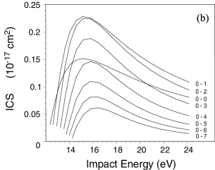
Figure 1: Total cross sections for excitation of $v=0,1,..,7$ vibrational levels of the $a^{3}\Sigma_{g}$ state of $\hbox{H}_{2}$.

The integral cross section for electron-vibrational excitation of $a\,^{3}\Sigma_{g}^{+}$ state of $\hbox{H}_{2}$ is plotted in fig. 1 for a number of values of $\alpha_{0},\alpha_{1},c,R$ (see [12]), which are regarded as constant in the range of interest.

7 Conclusion

Among the most important aspects of the paper are the development of the matrix ZRP theory, the calculation of the differential and integral cross sections for the electron-vibrational transitions, and investigation of the matrix ZRP possibilities. The nonoverlapping condition essentially simplifies a scattering problem solving. Thus, the determination of the multi-center matrix amplitude reduces to solving of the system (see Eqs. $(\ref{EQC}),(\ref{EQFmc})$) of integral equations. The number of scattering centers defines the number of equations in the system.

8 Acknowledgements

We acknowledge consultations of V. Ostrovsky and I. Yurova and discussions with J. Sienkiewicz and M. Zubek.

References

• [1] Fermi, E., 1936. Ric. Sci. 7, 13-52.
• [2] Breit, G., 1947. Phys. Rev. 71, 215-31.
• [3] Demkov, Yu., N., Ostrovsky, V., N., 1988. Zero-Range Potentials and their Applications in Atomic Physics, Plenum, New York.
• [4] Drukarev, G., F., Yurova, I., Yu., 1977. J. Phys. B: At. Mol. Phys. 10, 3551-8
• [5] Drukarev, G., F., 1978. Adv. Quantum Chem. 11, 251
• [6] Albeverio, S., Gesztesy, F., Høegh-Krohn, R., Holden, H., 1988. Solvable Models in Quantum Mechanics, Springer-Verlag, New York.
• [7] Huang, K., Yang, C., N., 1957. Phys. Rev. 105, 767
• [8] De Prunel$\acute{\hbox{e}}$, E., 1997, J. Phys. A: Math. Gen. 30, 7831-7848
• [9] Blatt, J., M., Weisskopf, V., F., 1952. Theoretical Nuclear Physics Wiley, New York, Section 2.3.C
• [10] Baltenkov, A., S., 2000. Phys. Lett. A, 286, 92-99.
• [11] Demkov, Yu., N., Ostrovsky, V., N., 1970. Sov. Phys.-JEPT, 32, 959-63
• [12] Leble, S., B., Yalunin, S., preprint quant-ph/0205110
• [13] Drozdov, S., I., 1955, Sov. Phys.-JETP, 1, 591-2
• [14] Chase, D., M., 1956. Phys. Rev., 104, 838-42
• [15] Oksyuk, Yu., D., 1965. Sov. Phys.-JETP, 49, 1261-73
• [16] Lane N., F., 1980. Rev. Mod. Phys., 52, 29-119
• [17] Varshalovich, D., A., Moskalev, A., N., Khersonskii, V., K., 1975. Quantum Theory of Angular Momentum, Nauka, Leningrad (in Russian)