Soliton back-action evading measurement using spectral filtering

Abstract

We report on a back-action evading (BAE) measurement of the photon number of fiber optical solitons operating in the quantum regime. We employ a novel detection scheme based on spectral filtering of colliding optical solitons. The measurements of the BAE criteria demonstrate significant quantum state preparation and transfer of the input signal to the signal and probe outputs exiting the apparatus, displaying the quantum-nondemolition (QND) behavior of the experiment.

]

I Introduction

Quantum theory allows for the measurement of an observable with arbitrarily high precision. In a back-action evading (BAE) measurement the back action inherent in the process of a quantum measurement is confined to the observable which is conjugate to the measured one [1]. If the initial state of a system is an eigenstate of the measurement operator, it is conserved and the BAE interaction is called quantum-nondemolition (QND). Initially designed for the detection of gravitational waves, the concept of QND measurements now is finding applications in the field of quantum information processing and communication [2].

Most BAE measurements have been carried out in quantum optics, where the quantum fluctuations are readily measurable. Quantitative criteria for QND and BAE experiments have been developed [3, 4, 5]. There are three physical systems in which BAE detection has been pursued experimentally: The $\chi^{(3)}$ interactions in optical fibers [6, 7] and in atoms [8], and the $\chi^{(2)}$ interaction in crystals [9]. The QND criteria were fulfilled in BAE detection with atomic systems ($\chi^{(3)}$) [10, 11] and $\chi^{(2)}$ interactions in crystals [12, 13, 14, 15, 16]. Repeated BAE measurements were reported using OPAs [17, 18] and a demonstration of principle using fiber optical pulses[19]. Despite their large potential for QND measurements [20, 21, 22, 23] fiber optical experiments have not previously been performed in the BAE regime [24, 7].

In this Paper we report experimental BAE results following a recently proposed fiber-optical back-action evading measurement scheme of the soliton photon number using spectral filtering of solitons [25].

Optical solitons are a natural physical system for implementing quantum communication concepts in fibers. Recently, they were used for EPR-pair beam generation [26]. Solitons are fiber optical pulses maintaining a stable shape due to a balance of group-velocity dispersion and nonlinearity. Moreover, after the collision of two solitons, the pulses recover energy, velocity and shape, and thus behave like particles. The nonstationary evolution of the soliton quantum fluctuations leads to remarkable effects. Quadrature squeezing was the first effect in a series of quantum optics experiments with solitons in fibers [27, 28]. In recent years amplitude squeezing of solitons using spectral filtering was discovered and explained as a multi mode quantum effect [29, 30, 31].

The technique of spectral filtering has since been generalized to a system of two colliding solitons [25]. A new theoretical proposal for BAE measurements was derived, in which a ”signal” soliton collides with a second ”probe” soliton. During the collision, the frequency of the probe becomes coupled to the photon number of the signal. A measurement of the probe frequency therefore gives a BAE readout of the signal photon number. Using this scheme we have obtained experimental BAE operation in the quantum regime. For the first time in fiber QND detection, the standard QND criteria are clearly fulfilled.

II Principle of the BAE measurement

The classical field evolution in a single-mode polarization preserving fiber is governed by the nonlinear Schrödinger equation (NLSE):

$$i\frac{\partial u}{\partial\xi}+\frac{1}{2}\frac{\partial^{2}u}{\partial\tau^{2}}+|u|^{2}u=0,$$ (1)

where $u$ is the slowly varying envelope of the electric field and $\xi$ and $\tau$ are time and space variables in a reference frame moving with the optical field [32]. $u$, $\xi$ and $\tau$ are given in soliton units [33]. The single pulse soliton solutions, i.e. the fundamental soliton of amplitude $A$ is given by [33]:

$$u(\tau,\xi)=A\,{\rm sech}(A(\tau+\Omega\xi))\exp(i(A^{2}-\Omega^{2})\xi/2-i\Omega\tau).$$ (2)

$\Omega$ is a dimensionless velocity of the soliton in units of inverse pulse length relative to the moving frame. At the same time $\Omega$ is a dimensionless center frequency of the soliton, because of the group-velocity dispersion. The collision of two fundamental solitons of equal amplitudes $A$, moving before the collision with $\pm\Omega_{0}$, is depicted in Figure 1.

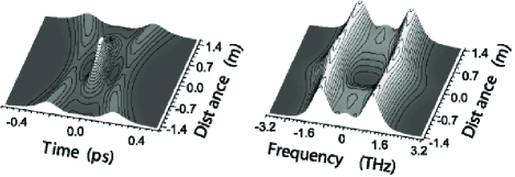
FIG. 1.: Evolution of the temporal and spectral power densities of two colliding solitons. Their initial frequency separation ($=$ relative velocity) in soliton units is $2\Omega_{0}=2.4$. The center of collision is at a distance $\xi=0$. The soliton period is $1.4$ m and in soliton units is given by: $\xi_{0}=\pi/2$.

As the solitons begin to overlap the enhanced intensity in the overlap region causes an attractive force and acceleration between the pulses. Therefore, the initial spectral separation and relative velocity of the solitons is transiently enhanced above the initial value of $2\Omega_{0}$. The spectral separation of the pulses, ”signal” and ”probe”, changes to $2\Omega_{0}+d\Omega_{S}+d\Omega_{P}$ and depends on the photon number of both solitons. Therefore, if the signal amplitude $A_{S}$ fluctuates around $A=\langle A_{S}\rangle$, the fluctuations $\Delta A_{S}=A_{S}-A$ induce fluctuations in the frequency $\Delta\Omega_{P}$ of the probe soliton at the collision center. If the soliton spectra do not overlap ($\Omega_{0}\gg 1$), the probe shift is given by [34]:

$$\langle d\Omega_{P}\rangle+\Delta\Omega_{P}=\frac{2A^{2}}{3\Omega_{0}}(1+\frac{\Delta A_{S}}{2A}+{\mathcal{O}}(\Delta A_{S}^{2}))$$ (3)

Towards the end of the collision the solitons recover their initial velocities (Fig.1).

The main idea of the novel BAE scheme is to measure the signal soliton amplitude fluctuations via the probe soliton frequency. The coupling is described classically by Eq. 3. Signal and probe solitons can be spectrally separated at the collision center (Fig.1). Then the frequency fluctuations $\Delta\Omega_{P}$ of the probe are read out with a spectral edge filter. The signal, which is the photon number, is preserved in the interaction as well as in the free fiber propagation, because of negligible fiber loss. The back action of the measurement perturbs the frequency and the phase of the signal pulse. For a quantum readout, the probe readout has to determine the signal intensity to better than the signal shot noise uncertainty. This measurement scheme was assessed by a detailed theoretical investigation accounting for the quantization of the field $u$. The result indicates that the signal is measured more precisely than within the shot noise and the scheme fulfills the QND criteria [25].

III Experimental realization

The experimental realization of the measurement requires three main steps: the pulse pair for the soliton collision has to be prepared and launched into the fiber. Then the detector is set up for the measurement of the conditional variance. Finally, the transfer coefficients are measured using an RF modulation on the signal input soliton. An overview of the experimental apparatus is presented in Fig. 2. The laser source is a $\rm{Cr}^{4+}$:YAG laser delivering 150-fs ${\rm sech}$-pulses at $\lambda=1.5\mu$m [35]. In the pulse former every pulse is spectrally split using a wavelength dependent beam splitter and retroreflected, double passing the beam splitter such that two pulses of different center wavelengths and with an adjustable temporal separation are obtained. They exhibit no relative phase noise or timing jitter in contrast to pulses from different laser sources. Figure 3(a) displays the two pulses after the pulse former. They have a spectral width of 12 nm and are separated by 14 nm.

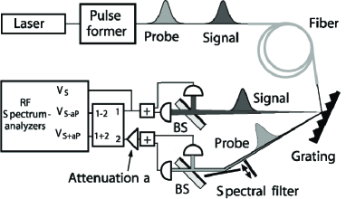
FIG. 2.: BAE apparatus for pulse pair generation, soliton collision and spectrally filtered probe detection (BS = beam splitter with $50\%$ reflection/transmission).

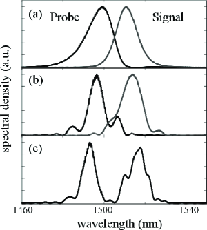
FIG. 3.: Signal and probe spectra out of the pulse former (a), after separate fiber propagation (b), and of a pulse collision (c) (relative phase of $\pi$).

The temporal width of the autocorrelation traces indicates pulse lengths of 200 fs. The time-bandwidth product is slightly increased above the Fourier limit (sech-shape assumed). In consequence, a weak dispersive wave evolves in the fiber in addition to the two solitons. The timing of the input pulses was adjusted to the output wave autocorrelation trace, taken for every measurement, such that the fiber end is exactly in the middle of the collision ($\xi=0$). As the signal to be measured in the BAE apparatus we consider the amplitude of the signal pulse after it is coupled into the fiber; therefore the coupling losses do not degrade the signal transfer through the BAE apparatus. Before the fiber the input pulse pair was shown to be shot-noise limited around 20 MHz to within $\pm 0.2$ dB. We used 6.3 m of polarization preserving single mode fiber (3M, FS-PM 7811) corresponding to 3.2 and 2.9 soliton periods [32] for the signal and probe solitons, respectively. The collision length, i.e. the length of the fiber where the solitons overlap within their (power) half width, is $L_{\rm coll}=3.2$ m. The solitons experience a nonlinear cross-phase shift of $\delta\phi_{NL}\approx 1.0$ rad. An output spectrum is shown in Fig. 3(c) and can be compared to the spectra of pulses which have propagated individually without collision (3(b)). The strong nonlinear coupling is clearly observable. The respective spectra shift about half a spectral width, $d\lambda\approx 5$ nm. The undulations in the spectra are caused by the weak dispersive wave. Due to the partial spectral overlap ($\Omega_{0}=1.2$) the soliton collision is phase dependent. This modifies the undulations, but the spectral shift changes by less than $5\%$.

The output pulses are spectrally dispersed using a grating (600 l/mm). Spectral filtering of the probe pulse is accomplished with a knife edge filter in the Fourier plane of the grating. Signal and probe pulses are separately directed onto two balanced two-port detectors (Epitaxx ETX500 photodiodes). The RF photocurrents are amplified after suppression of the repetition rate of the laser (163MHz). The sum current $I_{P}$ of the probe detector is attenuated with an attenuation $a$ and added to and subtracted from the signal sum current $I_{S}$. The shot-noise levels were determined by reading the DC photocurrents which display the average detected powers. They were carefully and repeatedly calibrated to the shot-noise level using the difference photocurrents of the balanced detectors which carry fluctuations of the signal and probe shot-noise levels.

The overall quantum efficiency for signal and probe detectors, including photodiode efficiencies, was measured to be 74.5% and 69.8%, respectively. The fiber loss ($\alpha<0.002{\rm dB/m}$) was neglected. Coupling losses from the fiber were minimized by means of an antireflection coated gradient-index lens.

The conditional variance and the transfer coefficients quantify the performance of a BAE experiment [3, 4, 5]. The conditional variance is a measure of the quantum state preparation ability of the apparatus. It can be written in terms of the photocurrents $I$ as:

$$V_{S/P}=\min_{a}\left(\frac{\langle(I_{S}+aI_{P})^{2}\rangle}{\langle I_{S,SN}^{2}\rangle}\right)$$ (4)

assuming $\langle I\rangle=0$. $I_{S}$ ($I_{P}$) measures the signal (probe) amplitude fluctuations, since the signal (probe) is directly detected. $I_{S,SN}$ denotes the corresponding shot noise.

IV Results

A measurement of the conditional variance is shown in Fig. 4. The three noise power levels of signal, sum and difference currents are recorded simultaneously on three RF spectrum analyzers. The photocurrent fluctuations are measured at $20$ MHz with a $300$ kHz resolution bandwidth. Thermal noise in the detector electronics is $6$ dB below the lowest detected noise level and is subtracted off in Fig. 4. The noise powers are quadratic functions of the attenuation $a$ as indicated by the parabolic fitting curve of Eq. 4. The displayed noise levels are normalized to the signal output shot noise. Signal and probe pulse are separated at $\lambda_{\rm sep}=1506$ nm after the fiber; the frequency low pass filter for the probe was applied at $\lambda_{\rm filt}=1490$ nm. At this position roughly $18\%$ of the probe pulse energy is filtered off and absorbed. The sum noise level in Fig. 4 decreases below the signal noise. This noise suppression corresponds to a strong negative photon number correlation of $C_{S/P}=-0.62\pm 0.03$, with the correlation coefficient defined as in [5, 25].

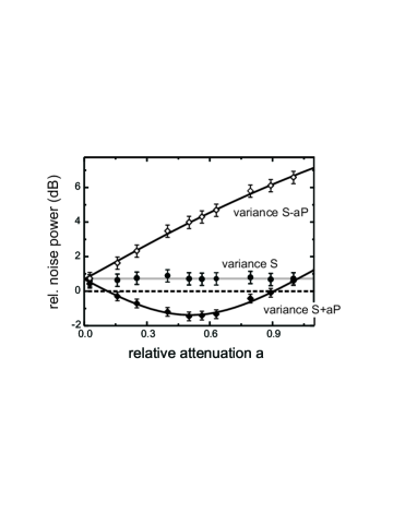
FIG. 4.: Photocurrent noise levels of combined photo currents, normalized to the signal output shot noise. Note that the combined noise decreases below signal output shot noise.

An anti-correlation is anticipated since an increase in the photon number of the signal causes an enhancement in the mutual spectral shift, in turn causing more losses in the probe pulse at the spectral filter. This correlation is not corrected for the finite quantum efficiencies of the detection apparatus. The noise reduction reaches $1.37\pm 0.3$ dB below the shot noise level of the signal, corresponding to a conditional variance of $V_{S/P}=0.73\pm 0.04$. The necessary condition for a QND experiment is $V<1$. This is clearly fulfilled.

The second important criterion for a QND measurement is the sum of the transfer coefficients. They describe the nondemolition property of the measurement with the transfer of the optical signal-to-noise ratio from the input to the output:

$${\rm T}_{S}=\frac{{\rm SNR}^{\rm out}_{S}}{{\rm SNR}^{\rm in}_{S}}=\frac{\langle(\Delta n_{S}^{\rm out})^{2}\rangle\langle n_{S}^{\rm in}\rangle}{\langle(\Delta n_{S}^{\rm in})^{2}\rangle\langle n_{S}^{\rm out}\rangle}$$ (5)

$${\rm T}_{P}=\frac{{\rm SNR}^{\rm out}_{P}}{{\rm SNR}^{\rm in}_{S}}=\frac{\langle(\Delta n_{P}^{\rm out})^{2}\rangle\langle n_{S}^{\rm in}\rangle}{\langle(\Delta n_{S}^{\rm in})^{2}\rangle\langle n_{P}^{\rm out}\rangle},$$ (6)

where $n$ denotes the photon numbers and $\Delta n$ is the modulation strength. Therefore we modulated the intensity of the signal beam with a $\mbox{LiTaO}_{3}$-electro-optic modulator at $20$ MHz before coupling into the fiber. The noise levels on and near to this frequency ($\sim 50$ kHz off the 20 MHz signal, recorded with a resolution bandwidth of 10 kHz.) were taken and the signal-to-noise ratio (${\rm SNR}$) for the signal input, the signal output and the probe output was determined [10]. If the probe soliton is absent, the unperturbed signal input exits the fiber (fiber damping and output coupling losses neglected). This way the signal input ${\rm SNR}$ is measured on the signal output detector. Therefore, the signal in- and output ${\rm SNR}$s can be measured with the same two-port detector. The signal transfer coefficient ${\rm T}_{S}$ is thus determined independently of detector efficiencies as the optical ${\rm SNR}$ transfer coefficient. The probe ${\rm SNR}$ is measured with the probe detector. As a consequence, the measured probe ${\rm SNR}$ has to be corrected for the small difference in signal and probe detector efficiencies of $6.3\%$. In a test, a weak phase modulation of the signal showed no ${\rm SNR}$ transfer to the probe. For an optimized filter, mainly the amplitude fluctuations of the signal couple to the detected part of the probe, despite the slight phase sensitivity of the collision. This also shows that the experiment is unaffected by thermal or quantum phase noise.

The best transfer coefficients measured were ${\rm T}_{S}+{\rm T}_{P}=0.99+0.63=1.62(\pm 0.15)$ at the filter settings of $\lambda_{\rm sep}=1504$ nm; $\lambda_{\rm filt}=1492$ nm. This was measured with an ${\rm SNR}$ of the incoming signal of 103, almost identical signal-out ${\rm SNR}$ and a probe-output ${\rm SNR}$ of 63. This high value of ${\rm T}_{S}+{\rm T}_{P}$ demonstrates the optical tapping property of the device.

Simultaneously optimizing the apparatus for both, a low conditional variance and high transfer coefficients, we observed $V_{S/P}=0.92\pm 0.05$ and ${\rm T}_{S}+{\rm T}_{P}=1.37\pm 0.13$ ($\lambda_{\rm sep}=1503$ nm; $\lambda_{\rm filt}=1490$ nm). This result clearly fulfills both the QND criteria. Depending on the relative phase of signal and probe as well as the filter positions ($\lambda_{\rm sep}$ and $\lambda_{\rm filt}$) the achieved transfer coefficients and conditional variances differ. The data obtained are presented in Fig.5. Stable results were obtained in all of the four quadrants. To achieve performance in the QND domain, we separated signal and probe at $1500$ nm$<\lambda_{\rm sep}<1506.5$ nm and low-pass filtered the probe at $1488$ nm$<\lambda_{\rm filt}<1490$ nm. The experimental results for $V_{S/P}$ and ${\rm T}_{S}+{\rm T}_{P}$ are not correlated. This suggests that additional noise is introduced to the solitons. Likely candidates are inter- and intra-soliton stimulated Raman scattering [36]. The Raman effect pumps photons towards the red and depletes the probe. This assumption is supported by an observed imbalance in the power of the output pulses of $\Delta P/P\approx\pm 8\%$ and by the observation of excess noise in the signal output (Fig.4). The effect decreases the observed signal transfer coefficient. A second perturbative effect is the evolving dispersive wave which modifies the quantum fluctuations significantly, because spectral correlations not only arise between the solitons, but also between them and the continuum [37, 38, 39, 40]. The use of longer pulses would reduce the Raman effect; the dispersive wave can be avoided with improved input pulse shaping.

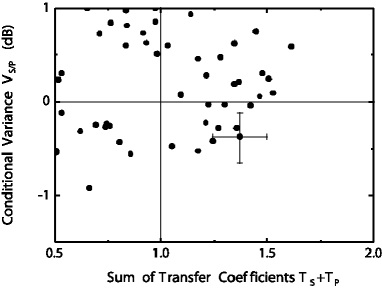
FIG. 5.: Data points obtained with the soliton collision experiment under different parameters, according to their transfer-coefficients and conditional variance.

A full QND experiment can be performed with repeated BAE measurements. When the signal is freely propagated after a first BAE interaction, the soliton will reshape with only little losses [25] and can be used in a second BAE measurement. A way to nearly eliminate residual radiation loss for cascaded BAE detection is the insertion of a second probe pulse in the center of the collision, prepared to complete the collision.

V Conclusion

In conclusion, we demonstrated a back-action evading measurement of the photon number based on the novel concept of spectral filtering. This new technique is robust against phase noise limiting previous experiments [7]. It requires merely two pulses since no phase reference pulse is needed and only direct detection is used for the BAE readout. The experiment showed large capacity for optical tapping as well as the capability for quantum state reduction. The idea of coupling to a completely different degree of freedom in the probe, neither conjugate nor identical to the signal observable may be utilized to improve BAE or QND measurements in fibers as well as in other $\chi^{(3)}$ and $\chi^{(2)}$ systems. Applications can be found, e. g. in quantum information [41] or weak absorption measurements [42]. Investigating the quantum properties of soliton collisions explores ultimate bounds in wavelength-division multiplexed optical transmission systems [33, 43].

REFERENCES

- [1] V. B. Braginsky, Y. I. Vorontsov, and K. S. Thorne, Science 209, 547 (1980).
- [2] G. Leuchs, C. Silberhorn, F. König, P. K. Lam, A. Sizmann, and N. Korolkova, in Quantum Information Theory with Continuous Variables, edited by S. L. Braunstein and A. K. Pati (Kluwer Academic, Dordrecht, 2002).
- [3] N. Imoto and S. Saito, Phys. Rev. A 39, 675 (1989).
- [4] M. J. Holland, M. J. Collett, D. F. Walls, and M. D. Levenson, Phys. Rev. A 42, 2995 (1990).
- [5] J. P. Poizat, J. F. Roch, and P. Grangier, Ann. Phys. Fr. 19, 2995 (1994).
- [6] M. D. Levenson, R. M. Shelby, M. Reid, and D. F. Walls, Phys. Rev. Lett. 57, 2473 (1986).
- [7] S. R. Friberg, S. Machida, and Y. Yamamoto, Phys. Rev. Lett. 69, 3165 (1992).
- [8] P. Grangier, J. F. Roch, and G. Roger, Phys. Rev. Lett. 66, 1418 (1991).
- [9] A. La Porta, R. E. Slusher, and B. Yurke, Phys. Rev. Lett. 62, 28 (1989).
- [10] J. P. Poizat and P. Grangier, Phys. Rev. Lett. 70, 271 (1993).
- [11] J.-F. Roch, K. Vigneron, P. Grelu, A. Sinatra, J.-P. Poizat, and P. Grangier, Phys. Rev. Lett. 78, 634 (1997).
- [12] J. A. Levenson, I. Abram, T. Rivera, P. Fayolle, J. C. Garreau, and P. Grangier, Phys. Rev. Lett. 70, 267 (1993).
- [13] S. F. Pereira, Z. Y. Ou, and H. J. Kimble, Phys. Rev. Lett. 72, 214 (1994).
- [14] S. Schiller, R. Bruckmeier, M. Schalke, K. Schneider, and J. Mlynek, Europhys. Lett. 36, 361 (1996).
- [15] R. Bruckmeier, K. Schneider, S. Schiller, and J. Mlynek, Phys. Rev. Lett. 78, 1243 (1997).
- [16] B. C. Buchler, P. K. Lam, H.-A. Bachor, U. L. Andersen, and T. C. Ralph, Phys. Rev. A 65, 011803(R) (2001).
- [17] K. Bencheikh, J. A. Levenson, P. Grangier, and O. Lopez, Phys. Rev. Lett. 75, 3422 (1995).
- [18] R. Bruckmeier, H. Hansen, and S. Schiller, Phys. Rev. Lett. 79, 1463 (1997).
- [19] S. R. Friberg, T. Mukai, and S. Machida, Phys. Rev. Lett. 84, 59 (2000).
- [20] H. A. Haus, K. Watanabe, and Y. Yamamoto, J. Opt. Soc. Am. B 6, 1138 (1989).
- [21] P. D. Drummond, J. Breslin, and R. M. Shelby, Phys. Rev. Lett. 73, 2837 (1994).
- [22] J. M. Courty, S. Spälter, F. König, A. Sizmann, and G. Leuchs, Phys. Rev. A 58, 1501 (1998).
- [23] V. V. Kozlov and D. A. Ivanov, Phys. Rev. A 65, 023812 (2002).
- [24] P. Grangier, J. A. Levenson, and J.-P. Poizat, Nature 396, 537 (1998).
- [25] F. König, M. A. Zielonka, and A. Sizmann, Phys. Rev. A 66, 013812 (2002).
- [26] C. Silberhorn, P. K. Lam, O. Weiß, F. König, N. Korolkova, and G. Leuchs, Phys. Rev. Lett. 86, 4267 (2001).
- [27] M. Rosenbluh and R. M. Shelby, Phys. Rev. Lett. 66, 153 (1991).
- [28] A. Sizmann and G. Leuchs, in The optical Kerr effect and quantum optics in fibers, Vol. XXXIV of Progress in Optics, edited by E. Wolf (Elsevier Publishers B. V., Amsterdam, 1999), p. 373.
- [29] M. J. Werner, Phys. Rev. A 54, R2567 (1996).
- [30] S. R. Friberg, S. Machida, M. J. Werner, A. Levanon, and T. Mukai, Phys. Rev. Lett. 77, 3775 (1996).
- [31] S. Spälter, N. Korolkova, F. König, A. Sizmann, and G. Leuchs, Phys. Rev. Lett. 81, 786 (1998).
- [32] G. P. Agrawal, Nonlinear Fiber Optics, 2 ed. (Academic Press, San Diego, 1995).
- [33] L. F. Mollenauer, S. G. Evangelides, and J. P. Gordon, IEEE J. Lightwave Tech. 9, 362 (1991).
- [34] This formula is an extension of a calculation from [33].
- [35] S. Spälter, M. Böhm, M. Burk, B. Mikulla, R. Fluck, I. Jung, G. Zhang, U. Keller, S. A., and G. Leuchs, Appl. Phys. B 65, 335 (1997).
- [36] S. Chi and S. Wen, Opt. Lett. 14, 1216 (1989).
- [37] A. Mecozzi and P. Kumar, Opt. Lett. 22, 1232 (1997).
- [38] D. Levandovsky, M. V. Vasilyev, and P. Kumar, Opt. Lett. 24, 43 (1999).
- [39] E. Schmidt, L. Knöll, D.-G. Welsch, M. Zielonka, F. König, and A. Sizmann, Phys. Rev. Lett. 85, 3801 (2000).
- [40] W. H. Loh, A. B. Grudinin, V. V. Afanasjev, and D. N. Payne, Opt. Lett. 19, 698 (1994).
- [41] S. L. Braunstein and A. K. Pati, Quantum Information Theory with Continuous Variables (Kluwer Academic, Dodrecht, 2001).
- [42] P. H. Souto Ribeiro, C. Schwob, A. Maître, and C. Fabre, Opt. Lett. 22, 1893 (1997).
- [43] A. Sizmann, F. König, M. A. Zielonka, R. Steidl, and T. Rechtenwald, in Massive WDM and TDM Soliton Transmission Systems, edited by A. Hasegawa (Kluwer Academic Publishers, Dodrecht, The Netherlands, 2000), p. 289.