Decoherence of entangled kaons and its connection to entanglement measures

Abstract

We study the time evolution of the entangled kaon system by considering the Liouville - von Neumann equation with an additional term which allows for decoherence. We choose as generators of decoherence the projectors to the 2-particle eigenstates of the Hamiltonian. Then we compare this model with the data of the CPLEAR experiment and find in this way an upper bound on the strength $\lambda$ of the decoherence. We also relate $\lambda$ to an effective decoherence parameter $\zeta$ considered previously in literature. Finally we discuss our model in the light of different measures of entanglement, i.e. the von Neumann entropy $S$, the entanglement of formation $E$ and the concurrence $C$, and we relate the decoherence parameter $\zeta$ to the loss of entanglement: $1-E$.

PACS numbers: 14.40.Aq, 03.65.Bz, 03.67.-a
Keywords: entangled kaons, nonlocality, decoherence, entropy, entanglement of formation, quantum information

I Introduction

Particle physics has become an interesting testing ground for fundamental questions of quantum mechanics (QM). For instance, QM versus local realistic theories [1, 2, 3, 4] and Bell inequalities [5, 6, 7, 8, 9, 10, 11, 12] have been tested. Furthermore, possible deviations from the quantum mechanical time evolution have been studied, particularly in the neutral K-meson system [13, 14, 15, 16, 17, 18, 19] and B-meson system [20, 21, 22, 23, 24]. Recently also neutrino oscillations have become of interest in this connection [25].

In this paper we concentrate on possible decoherence effects arising due to some interaction of the system with its “environment”. Sources for “standard” decoherence effects are the strong interaction scatterings of kaons with nucleons, the weak interaction decays and the noise of the experimental setup. “Nonstandard” decoherence effects result from a fundamental modification of QM and can be traced back to the influence of quantum gravity [26, 27, 28] – quantum fluctuations in the space-time structure on the Planck mass scale – or to dynamical state reduction theories [29, 30, 31, 32], and arise on a different energy scale. However, we do not pursue further the reasons for decoherence effects, rather we want to develop a specific model of decoherence and quantify the strength $\lambda$ of such possible effects with the help of data of existing experiments.

For our model we focus on entangled massive particles moving apart in their center of mass system, in particular on the $K^{0}\bar{K}^{0}\;$system, where the strangeness $S=+,-$ plays the role of spin “up” and “down” (for details see Ref. [33]). We consider here the famous EPR-like (Einstein, Podolsky, Rosen) scenario, as described by Bell [34] for spin-$1/2$ particles, where the initial spin singlet state evolves in time and after macroscopic separation the strangeness of the left and right moving particle is measured. In contrast to other concepts in the literature we introduce decoherence in the time evolution of the 2-particle entangled state which becomes stronger with increasing distance between the two particles, whereas for the 1-particle state we assume the usual quantum mechanical time evolution.

Then we compare our model of decoherence with the experimental data of the CPLEAR experiment performed at CERN [35] and find an upper bound on possible decoherence. We also can relate our model to an effective decoherence parameter $\zeta$, introduced previously in literature, which quantifies the spontaneous factorization of the wavefunction into product states (Furry–Schrödinger hypothesis [36, 46]).

Finally we discuss our model within concepts of quantum information, where entanglement is quantified by certain measures. We can connect directly the amount of decoherence of the $K^{0}\bar{K}^{0}\;$system parametrized by $\lambda$ or $\zeta$ with the loss of entanglement expressed in terms of the concurrence or in terms of entanglement of formation. The numerics for the information loss, the von Neumann entropy, and the entanglement loss of the evolving $K^{0}\bar{K}^{0}\;$system we illustrate in Fig.1.

II The model

Let us begin our decoherence discussion with the 1-particle kaon system as an introduction. Then we proceed to the case of two entangled neutral kaons and compare it with experimental data.

A The 1-particle case

We discuss the model of decoherence in a 2-dimensional Hilbert space $\mathcal{H}=\mathbf{C}^{2}$ and consider the usual non-Hermitian “effective mass” Hamiltonian $H$ which describes the decay properties and the strangeness oscillations of the kaons. The mass eigenstates, the short lived $|K_{S}\rangle$ and long lived $|K_{L}\rangle$ states, are determined by

$$H\;|K_{S,L}\rangle\;=\;\lambda_{S,L}\;|K_{S,L}\rangle\qquad\textrm{with}\quad\lambda_{S,L}\;=\;m_{S,L}-\frac{i}{2}\Gamma_{S,L}\,,$$ (1)

with $m_{S,L}$ and $\Gamma_{S,L}$ being the corresponding masses and decay widths. For our purpose $\mathcal{CP}\;$invariance is assumed, i.e. the $\mathcal{CP}\;$eigenstates $|K_{1}^{0}\rangle,|K_{2}^{0}\rangle$ are equal to the mass eigenstates

$$|K_{1}^{0}\rangle\equiv|K_{S}\rangle,\quad|K_{2}^{0}\rangle\equiv|K_{L}\rangle,\qquad\textrm{and}\quad\langle K_{S}|K_{L}\rangle=0\;.$$ (2)

As a starting point for our model of decoherence we consider the Liouville - von Neumann equation with the Hamiltonian (1) and allow for decoherence by adding a so-called dissipator $D[\rho]$, so that the time evolution of the density matrix $\rho$ is governed by a master equation of the form

$$\frac{d\rho}{dt} = -iH\rho+i\rho H^{\dagger}-D[\rho]\;.$$ (3)

For the term $D[\rho]$ we choose the following ansatz (as in Ref. [37])

$$D[\rho]\;=\;\lambda\,\big{(}P_{S}\rho P_{L}+P_{L}\rho P_{S}\big{)}\;=\;\frac{\lambda}{2}\sum_{j=S,L}\big{[}P_{j},[P_{j},\rho]\big{]}\;,$$ (4)

where $P_{j}\;=\;|K_{j}\rangle\langle K_{j}|$ ($j=S,L$) represent the projectors to the eigenstates of the Hamiltonian and the decoherence parameter $\lambda$ is positive, $\lambda\geq 0$.

Apart from its simplicity ansatz (4) has the following nice features:

1. It generates a completely positive map since it is a special case of Lindblad’s general structure [38]

   $$D[\rho]\;=\;\frac{1}{2}\sum_{j}(A^{\dagger}_{j}A_{j}\;\rho+\rho A^{\dagger}_{j}A_{j}-2A_{j}\rho A_{j}^{\dagger})$$ (5)

   if we identify $A_{j}=\sqrt{\lambda}\,P_{j}\;,\;j=S,L$.

   Equivalently, it is a special form of the Gorini-Kossakowski-Sudarshan [39] expression (see, e.g., Ref. [40]).

2. It conserves energy in case of a Hermitian Hamiltonian since $[P_{j},H]=0$ (see, e.g. Ref. [41]).

3. The von Neumann entropy $S(\rho)=-\mathrm{Tr}(\rho\ln\rho)$ is not decreasing as a function of time since $P_{j}^{\dagger}=P_{j}$, thus $A_{j}^{\dagger}=A_{j}$ in our case, which is a theorem due to Narnhofer and Benatti [42].

With choice (4) the time evolution (3) decouples for the components of $\rho$ which are defined by

$$\rho(t)\;=\sum_{i,j=S,L}\rho_{ij}(t)\,|K_{i}\rangle\langle K_{j}|\,,$$ (6)

and we obtain

$$\rho_{SS}(t) = \rho_{SS}(0)\cdot e^{-\Gamma_{S}t}$$ (7)

$$\rho_{LL}(t) = \rho_{LL}(0)\cdot e^{-\Gamma_{L}t}$$ (8)

$$\rho_{LS}(t) = \rho_{LS}(0)\cdot e^{-i\Delta mt-\Gamma t-\lambda t}$$ (9)

with $\Delta m=m_{L}-m_{S}$ and $\Gamma=\frac{1}{2}(\Gamma_{S}+\Gamma_{L})$. Only the off-diagonal elements are effected by our model of decoherence. Before discussing further the model we now proceed to the 2-particle system.

B The 2-particle case

In the case of two entangled neutral kaons we make the following identification

$$|e_{1}\rangle\;=\;|K_{S}\rangle_{l}\otimes|K_{L}\rangle_{r}\qquad\textrm{and}\qquad|e_{2}\rangle\;=\;|K_{L}\rangle_{l}\otimes|K_{S}\rangle_{r}\;,$$ (10)

and we consider – as common – the total Hamiltonian as a tensor product of the 1-particle Hilbert spaces: $H=H_{l}\otimes\mathbf{1}_{r}+\mathbf{1}_{l}\otimes H_{r}$, where $l$ denotes the left-moving and $r$ the right-moving particle. Then the initial quasispin singlet state

$$|\psi^{-}\rangle = \frac{1}{\sqrt{2}}\biggl{\{}|e_{1}\rangle-|e_{2}\rangle\biggr{\}}\;,$$ (11)

is equivalently given by the density matrix

$$\rho(0)\;=\;|\psi^{-}\rangle\langle\psi^{-}|\;=\;\frac{1}{2}\biggl{\{}|e_{1}\rangle\langle e_{1}|+|e_{2}\rangle\langle e_{2}|-|e_{1}\rangle\langle e_{2}|-|e_{2}\rangle\langle e_{1}|\biggr{\}}\;.$$ (12)

Following the considerations of the 1-particle case we find that the time evolution given by (3) with our choice (4), where now the operators $P_{j}\;=\;|e_{j}\rangle\langle e_{j}|$ ($j=1,2$) project to the eigenstates of the 2-particle Hamiltonian $H$, also decouples

$$\rho_{11}(t) = \rho_{11}(0)\;e^{-2\Gamma t}$$ (13)

$$\rho_{22}(t) = \rho_{22}(0)\;e^{-2\Gamma t}$$ (14)

$$\rho_{12}(t) = \rho_{12}(0)\,e^{-2\Gamma t-\lambda t}\;.$$ (15)

Consequently we obtain for the time-dependent density matrix

$$\rho(t)\;=\;\frac{1}{2}e^{-2\Gamma t}\biggl{\{}|e_{1}\rangle\langle e_{1}|+|e_{2}\rangle\langle e_{2}|-e^{-\lambda t}\big{(}\,|e_{1}\rangle\langle e_{2}|+|e_{2}\rangle\langle e_{1}|\,\big{)}\biggr{\}}\;.$$ (16)

The decoherence arises through the factor $e^{-\lambda t}$ which only effects the off-diagonal elements. It means that for $t>0$ and $\lambda\not=0$ the density matrix $\rho(t)$ does not correspond to a pure state anymore (for further discussion, see Section IV).

Note that the assumption of $\mathcal{CP}\;$invariance, Eq.(2), – which is sufficient for our purpose – implying $\langle e_{1}|e_{2}\rangle=0$, is crucial. Otherwise we would have a time evolution into the full 4-dimensional Hilbert space of states.

C Bounds from experimental data

In order to obtain information on possible values of $\lambda$ we compare our model of decoherence with data of the CPLEAR experiment performed at CERN [35]. We have the following point of view. The 2-particle density matrix follows the time evolution given by Eq.(3) with the Lindblad generators $A_{j}=\sqrt{\lambda}\;|e_{j}\rangle\langle e_{j}|$ and undergoes thereby some decoherence. We measure the strangeness content $S$ of the left-moving particle at time $t_{l}$ and of the right-moving particle at time $t_{r}$. For sake of definiteness we choose $t_{r}\leq t_{l}$. For times $t_{r}\leq t\leq t_{l}$ we have a 1-particle state which evolves exactly according to QM, i.e. no further decoherence is picked up.

Mathematically, the measurement of the strangeness content, i.e. the right-moving particle being a $K^{0}$ or a $\bar{K}^{0}$ at time $t_{r}$, is obtained by

$$\mathrm{Tr}_{r}\{\mathbf{1}_{l}\otimes|S^{{}^{\prime}}\rangle\langle S^{{}^{\prime}}|_{r}\;\;\rho(t_{r})\} \equiv \rho_{l}(t=t_{r};t_{r})\;,$$ (17)

with strangeness $S^{{}^{\prime}}=+,-$ and $|+\rangle=|K^{0}\rangle$, $|-\rangle=|\bar{K}^{0}\rangle$. Consequently, $\rho_{l}(t;t_{r})$ for times $t\geq t_{r}$ is the 1-particle density matrix for the left-moving particle and evolves as a 1-particle state according to pure QM. At $t=t_{l}$ the strangeness content ($S=+,-$) of the second particle is measured and we finally have the probability

$$P_{\lambda}(S,t_{l};S^{{}^{\prime}},t_{r}) = \mathrm{Tr}_{l}\{|S\rangle\langle S|_{l}\;\;\rho_{l}(t_{l};t_{r})\}\;.$$ (18)

Explicitly, we find the following results for the like- and unlike-strangeness probabilities

$$P_{\lambda}(K^{0},t_{l};K^{0},t_{r})\;=\;P_{\lambda}(\bar{K}^{0},t_{l};\bar{K}^{0},t_{r})\;=$$ (19)

$$= \frac{1}{8}\biggl{\{}e^{-\Gamma_{S}t_{l}-\Gamma_{L}t_{r}}+e^{-\Gamma_{L}t_{l}-\Gamma_{S}t_{r}}-e^{-\lambda t_{r}}\;2\cos(\Delta m\Delta t)\cdot e^{-\Gamma(t_{l}+t_{r})}\biggr{\}}$$ (20)

$$P_{\lambda}(K^{0},t_{l};\bar{K}^{0},t_{r})\;=\;P_{\lambda}(\bar{K}^{0},t_{l};K^{0},t_{r})\;=$$ (21)

$$= \frac{1}{8}\biggl{\{}e^{-\Gamma_{S}t_{l}-\Gamma_{L}t_{r}}+e^{-\Gamma_{L}t_{l}-\Gamma_{S}t_{r}}+e^{-\lambda t_{r}}\;2\cos(\Delta m\Delta t)\cdot e^{-\Gamma(t_{l}+t_{r})}\biggr{\}}\;,$$ (22)

with $\Delta t=t_{l}-t_{r}$.

Note that at equal times $t_{l}=t_{r}=t$ the like-strangeness probabilities

$$P_{\lambda}(K^{0},t;K^{0},t)\;=\;P_{\lambda}(\bar{K}^{0},t;\bar{K}^{0},t)\;=\;\frac{1}{4}\;e^{-2\Gamma t}\;(1-e^{-\lambda t})$$ (23)

do not vanish, in contrast to the quantum mechanical EPR-correlation.

The asymmetry of the probabilities is directly sensitive to the interference term and has been measured by the CPLEAR collaboration [35]. For pure QM we have

$$A^{QM}(\Delta t)=$$ (24)

$$= \frac{P(K^{0},t_{l};\bar{K}^{0},t_{r})+P(\bar{K}^{0},t_{l};K^{0},t_{r})-P(K^{0},t_{l};K^{0},t_{r})-P(\bar{K}^{0},t_{l};\bar{K}^{0},t_{r})}{P(K^{0},t_{l};\bar{K}^{0},t_{r})+P(\bar{K}^{0},t_{l};K^{0},t_{r})+P(K^{0},t_{l};K^{0},t_{r})+P(\bar{K}^{0},t_{l};\bar{K}^{0},t_{r})}$$ (25)

$$= \;\frac{\cos(\Delta m\Delta t)}{\cosh(\frac{1}{2}\Delta\Gamma\Delta t)}\;,$$ (26)

with $\Delta\Gamma=\Gamma_{L}-\Gamma_{S}$, and for our decoherence model we find by inserting the probabilities (19)

$$A^{\lambda}(t_{l},t_{r}) = \frac{\cos(\Delta m\Delta t)}{\cosh(\frac{1}{2}\Delta\Gamma\Delta t)}\cdot e^{-\lambda\min{\{t_{l},t_{r}\}}}\;=\;A^{QM}(\Delta t)\cdot e^{-\lambda\min{\{t_{l},t_{r}\}}}\;.$$ (27)

Thus the decoherence effect, simply given by the factor $e^{-\lambda\min{\{t_{l},t_{r}\}}}$, depends only – due to our philosophy – on the time of the first measured kaon, in our case: $\min{\{t_{l},t_{r}\}}=t_{r}$.

Comparing now our model with the results of the CPLEAR experiment [35] we recall that the experimental set-up has two configurations: In the first configuration both kaons propagate $2cm$, in the second one kaon propagates $2cm$ and the other kaon $7cm$ until they are measured by an absorber.

Fitting the decoherence parameter $\lambda$ by comparing the asymmetry (27) with the experimental data [35] we find, when averaging over both configurations, the following bounds on $\lambda$

$$\bar{\lambda}\;=\;(1.84^{+2.50}_{-2.17})\cdot 10^{-12}\;\textrm{MeV}\quad\textrm{and}\quad\bar{\Lambda}\;=\;\frac{\bar{\lambda}}{\Gamma_{S}}\;=\;0.25^{+0.34}_{-0.32}\;.$$ (28)

The results (28) are certainly compatible with QM ($\lambda=0$), nevertheless, the experimental data allow an upper bound $\bar{\lambda}_{up}=4.34\cdot 10^{-12}\;\textrm{MeV}$ for possible decoherence in the entangled $K^{0}\bar{K}^{0}\;$  system.

The results (28) can be compared with the analogous investigation of the entangled $B^{0}\bar{B}^{0}$ system [37], which gives $\lambda_{B}=(-47\pm 76)\cdot 10^{-12}\;\textrm{MeV}$. Thus we find that the bounds (28) of the $K^{0}\bar{K}^{0}\;$system are an order of magnitude more restrictive.

III Connection to a phenomenological model

There exists a one-to-one correspondence between the model of decoherence (3) and a phenomenological model [22, 43, 44, 45] where the decoherence is introduced by multiplying the interference term of the transition amplitude by the factor $(1-\zeta)$. The quantity $\zeta$ is called the effective decoherence parameter. Our initial state is again the spin singlet state $|\psi^{-}\rangle$ which is given by the mass eigenstate representation (11) then we get for the like-strangeness probability

$$P(K^{0},t_{l};K^{0},t_{r})\;=\;||\langle K^{0}|_{l}\otimes\langle K^{0}|_{r}\;|\psi^{-}(t_{l},t_{r})\rangle||^{2}\quad\longrightarrow\quad P_{\zeta}(K^{0},t_{l};K^{0},t_{r})=$$ (29)

$$= \frac{1}{2}\biggl{\{}e^{-\Gamma_{S}t_{l}-\Gamma_{L}t_{r}}|\langle K^{0}|K_{S}\rangle_{l}|^{2}\;|\langle K^{0}|K_{L}\rangle_{r}|^{2}+e^{-\Gamma_{L}t_{l}-\Gamma_{S}t_{r}}|\langle K^{0}|K_{L}\rangle_{l}|^{2}\;|\langle K^{0}|K_{S}\rangle_{r}|^{2}$$ (32)

$$-2\underbrace{(1-\zeta)}\;\mathrm{Re}\{\langle K^{0}|K_{S}\rangle_{l}^{*}\langle K^{0}|K_{L}\rangle_{r}^{*}\langle K^{0}|K_{L}\rangle_{l}\langle K^{0}|K_{S}\rangle_{r}\;e^{-i\Delta m\Delta t}\}\cdot e^{-\Gamma(t_{l}+t_{r})}\biggr{\}}$$

modification

$$= \frac{1}{8}\biggl{\{}e^{-\Gamma_{S}t_{l}-\Gamma_{L}t_{r}}+e^{-\Gamma_{L}t_{l}-\Gamma_{S}t_{r}}-2\underbrace{(1-\zeta)}\cos(\Delta m\Delta t)\cdot e^{-\Gamma(t_{l}+t_{r})}\biggr{\}}\;,$$ (34)

modification

and the unlike-strangeness probability just changes the sign of the interference term.

The value $\zeta=0$ corresponds to pure QM and $\zeta=1$ to total decoherence or spontaneous factorization of the wave function, which is commonly known as Furry–Schrödinger hypothesis [36, 46]. The effective decoherence parameter $\zeta$, introduced in this way “by hand”, interpolates continuously between these two limits and represents a measure for the amount of decoherence which results in a loss of entanglement of the total quantum state (we come back to this point in Section IV).

Calculating the asymmetry of the strangeness events with the probabilities (29) we obtain

$$A^{\zeta}(t_{l},t_{r})\;=\;A^{QM}(\Delta t)\cdot\big{(}\,1-\zeta(t_{l},t_{r})\,\big{)}\;.$$ (35)

When we compare now the two approaches, i.e. Eq.(27) with Eq.(35), we find the formula

$$\zeta(t_{l},t_{r})\;=\;1-e^{-\lambda\min{\{t_{l},t_{r}\}}}\;.$$ (36)

Of course, the values (28) are in agreement with the corresponding $\zeta$ values (averaged over both experimental setups): $\bar{\zeta}\,=\,0.13^{+0.16}_{-0.15}\,$, as derived in Refs. [43, 47].

We consider the decoherence parameter $\lambda$ to be the fundamental constant, whereas the value of the effective decoherence parameter $\zeta$ depends on the time when a measurement is performed. In the time evolution of the state $|\psi^{-}\rangle$, Eq.(11), represented by the density matrix (16), we have the relation

$$\zeta(t)\;=\;1-e^{-\lambda t}\;,$$ (37)

which after the measurement of the left- and right moving particles at $t_{l}$ and $t_{r}$ turns into formula (36), when decoherence is implemented at the 2-particle level.

Our model can be compared with the case where decoherence in the time evolution (3) happens at a 1-particle level and is transferred to the 2-particle level by a tensor product of the 1-particle Hilbert spaces [18]. Using the same structure of the decoherence term (4), where now the operators project to the 1-particle states instead of states (10), we obtain the relation

$$\zeta(t_{l},t_{r})\;=\;1-e^{-\lambda\,(t_{l}+t_{r})}\;.$$ (38)

Here the parameter $\zeta$ depends explicitly on both times $t_{l}$ and $t_{r}$, the “eigentimes” of the left- and right-moving kaon, instead of one time $\min{\{t_{l},t_{r}\}}$, the time of the system when the first kaon is measured.

Measuring the strangeness content of the entangled kaons at definite times we have the possibility to distinguish experimentally these two models (36) and (38) on the basis of time dependent event rates. Indeed, it would be of high interest to measure in future experiments the asymmetry of the strangeness events for several different times, in order to confirm the time dependence of the decoherence effect. In fact, such a possibility is now offered in the B-meson system. Entangled $B^{0}\bar{B}^{0}$ pairs are created with high density at the asymmetric B-factories and identified by the detectors BELLE at KEK-B (see e.g. Refs. [48, 49]) and BABAR at PEP-II (see e.g. Refs. [50, 51]) with a high resolution at different distances or times.

IV Decoherence and entanglement loss

The term $D[\rho]$ in the master equation (3) is usually called dissipative term or dissipator (see, e.g., Ref. [52]). In general, $D[\rho]$ describes 2 phenomena occurring in an open quantum system $S$, namely decoherence and dissipation. When the system $S$ interacts with the environment $E$ the initially product state evolves into entangled states of $S+E$ in the course of time [53, 54]. It leads to mixed states in $S$ – what means decoherence – and to an energy exchange between $S$ and $E$ – what is called dissipation.

The decoherence destroys the occurrence of longrange quantum correlations by suppressing the off-diagonal elements of the density matrix in a given basis and leads to an information transfer from $S$ to $E$.

In general, both effects are present, however, decoherence acts on a much shorter time scale [53, 55, 56, 57] than dissipation and is the more important effect in quantum information processes.

Our model describes decoherence and not dissipation. The increase of decoherence of the initially totally entangled $K^{0}\bar{K}^{0}\;$system as time evolves means on the other hand a decrease of entanglement of the system. This loss of entanglement we can quantify and visualize explicitly.

In the field of quantum information the entanglement of a state is quantified by introducing certain measures. In this connection the entropy plays a fundamental role, which measures “somehow” the degree of uncertainty of a quantum state. A common measure is the von Neumann entropy function $S$, the entanglement of formation $E$ and the concurrence $C$.

A Von Neumann entropy

Since we are only interested in the effect of decoherence, we want to properly normalize the state (16) in order to compensate the decay property of the non-Hermitian Hamiltonian $H$

$$\rho_{N}(t) = \frac{\rho(t)}{\mathrm{Tr}\rho(t)}\;.$$ (39)

Then von Neumann’s entropy function for the state (39) gives

$$S\big{(}\rho_{N}(t)\big{)} = -\mathrm{Tr}\{\rho_{N}(t)\log_{2}\rho_{N}(t)\}$$ (40)

$$= -\frac{1-e^{-\lambda t}}{2}\log_{2}\frac{1-e^{-\lambda t}}{2}-\frac{1+e^{-\lambda t}}{2}\log_{2}\frac{1+e^{-\lambda t}}{2}\;.$$ (41)

At the time $t=0$ the entropy is zero, there is no uncertainty in the system, the quantum state is pure and maximally entangled. For $t>0$ the entropy gets nonzero, increases and approaches the value $1$ for $t\to\infty$. Hence the state becomes more and more mixed. Mixed states provide only partial information about the system, and the entropy measures how much of the maximal information is missing (see, e.g., Ref. [58]). In Fig.1 the von Neumann entropy $S(\rho_{N}(t))$ is plotted for the mean value and upper bound of the decoherence parameter $\lambda$, Eq.(28), as determined from the CPLEAR experiment [35].

Let us consider next the reduced density matrices of the subsystems, i.e. the propagating kaons on the left $l$ and right $r$ hand side

$$\rho^{\,l}_{N}(t)=\mathrm{Tr}_{r}\{\rho_{N}(t)\}\quad\textrm{and}\quad\rho^{\,r}_{N}(t)=\mathrm{Tr}_{l}\{\rho_{N}(t)\}\;.$$ (42)

Then the uncertainty in the subsystem $l$ before the subsystem $r$ is measured is given by the von Neumann entropy $S(\rho^{\,l}_{N}(t))$ of the corresponding reduced density matrix $\rho^{\,l}_{N}(t)$ (and alternatively we can replace $l\to r$). In our case we find

$$S\big{(}\rho^{\,l}_{N}(t)\big{)}=S\big{(}\rho^{\,r}_{N}(t)\big{)}=1\quad\forall\;t\geq 0\;.$$ (43)

We see that the reduced entropies are independent of $\lambda$. The correlation stored in the composite system is, with increasing time, lost into the environment – what is expected intuitively – and not into the subsystems, i.e. the individual kaons.

Note that because of our chosen normalization (39) the effects seen are only due to the introduced decoherence via the term $D[\rho]$ (4) and not due to the decay of the system.

B Lack of separability

For the subsequent considerations it is convenient to recall the “quasispin” picture for the $K^{0}\bar{K}^{0}\;$system (see, e.g., Ref. [8]) in order to express the formulae in terms of Pauli spin matrices. Then the projection operators to the mass eigenstates represent the spin projection operators “up” and “down”

$$P_{S} = |K_{S}\rangle\langle K_{S}|\;=\;\sigma_{\uparrow}\;=\;\frac{1}{2}\,(\mathbf{1}+\sigma_{z})\;=\;\left(\begin{array}[]{cc}1&0\\ 0&0\\ \end{array}\right)\;,$$ (46)

$$P_{L} = |K_{L}\rangle\langle K_{L}|\;=\;\sigma_{\downarrow}\;=\;\frac{1}{2}\,(\mathbf{1}-\sigma_{z})\;=\;\left(\begin{array}[]{cc}0&0\\ 0&1\\ \end{array}\right)\;,$$ (49)

and the transition operators are the “spin-ladder” operators

$$P_{SL} = |K_{S}\rangle\langle K_{L}|\;=\;\sigma_{+}\;=\;\frac{1}{2}\,(\sigma_{x}+i\,\sigma_{y})\;=\;\left(\begin{array}[]{cc}0&1\\ 0&0\\ \end{array}\right)\;,$$ (52)

$$P_{LS} = |K_{L}\rangle\langle K_{S}|\;=\;\sigma_{-}\;=\;\frac{1}{2}\,(\sigma_{x}-i\,\sigma_{y})\;=\;\left(\begin{array}[]{cc}0&0\\ 1&0\\ \end{array}\right)\;.$$ (55)

With help of these spin matrices the density matrix (39) can be expressed by

$$\rho_{N}(t)\,=\,\frac{1}{2}\big{\{}\sigma_{\uparrow}\otimes\sigma_{\downarrow}+\sigma_{\downarrow}\otimes\sigma_{\uparrow}\,-\,e^{-\lambda t}\,[\sigma_{+}\otimes\sigma_{-}+\sigma_{-}\otimes\sigma_{+}]\big{\}}\;,$$ (56)

or by

$$\rho_{N}(t)\,=\,\frac{1}{4}\big{\{}\mathbf{1}-\sigma_{z}\otimes\sigma_{z}\,-\,e^{-\lambda t}\,[\sigma_{x}\otimes\sigma_{x}+\sigma_{y}\otimes\sigma_{y}]\big{\}}\;,$$ (57)

which at $t=0$ coincides with the well-known expression for the pure spin singlet state $\rho_{N}(t=0)\,=\,\frac{1}{4}\,(\mathbf{1}-\vec{\sigma}\otimes\vec{\sigma})$; see, e.g., Ref. [59]. Operators (56), (57) can be nicely written as $4\times 4$ matrix

$$\rho_{N}(t)\;=\;\frac{1}{2}\left(\begin{array}[]{cccc}0&0&0&0\\ 0&1&-e^{-\lambda t}&0\\ 0&-e^{-\lambda t}&1&0\\ 0&0&0&0\\ \end{array}\right)\;.$$ (62)

It is also illustrative to choose for the density matrix $\rho_{N}(t)$ another basis, the socalled “Bell basis”

$$\rho^{\mp}\;=\;|\psi^{\mp}\rangle\langle\psi^{\mp}|\qquad\textrm{and}\qquad\omega^{\mp}\;=\;|\phi^{\mp}\rangle\langle\phi^{\mp}|\;,$$ (63)

with $|\psi^{-}\rangle$ given by Eq.(11) and $|\psi^{+}\rangle$ by

$$|\psi^{+}\rangle = \frac{1}{\sqrt{2}}\biggl{\{}|e_{1}\rangle+|e_{2}\rangle\biggr{\}}\;.$$ (64)

The states $|\phi^{\mp}\rangle=\frac{1}{\sqrt{2}}(|\uparrow\uparrow\rangle\mp|\downarrow\downarrow\rangle)$ (in spin notation) do not contribute here. Then we are led to the following proposition.

Proposition: The state represented by the density matrix $\rho_{N}(t)$ (39) becomes mixed for $0<t<\infty$ but remains entangled. Separability is achieved asymptotically $t\to\infty$ with the weight $e^{-\lambda t}$. Explicitly, $\rho_{N}(t)$ is the following mixture of the Bell states $\rho^{-}$ and $\rho^{+}\,$:

$$\rho_{N}(t)\;=\;\frac{1}{2}\big{(}1+e^{-\lambda t}\big{)}\,\rho^{-}\;+\;\frac{1}{2}\big{(}1-e^{-\lambda t}\big{)}\,\rho^{+}\;.\\$$ (65)

Proof:

• Diagonalizing matrix (62) we find $\big{\{}\frac{1}{2}\big{(}1+e^{-\lambda t}\big{)},\frac{1}{2}\big{(}1-e^{-\lambda t}\big{)},0,0\big{\}}$, the eigenvalues together with the eigenvectors $\rho^{-}$ and $\rho^{+}\,$, which proves Eq.(65). For $t=0$ the matrix $\rho_{N}(0)$ is a projector to a 1-dimensional subspace: $\{1,0,0,0\}$, the Bell state $\rho^{-}\,$, so the state is pure. For $0<t<\infty$ the matrix $\rho_{N}(t)$ is no longer a projector, thus the state is mixed. The state becomes asymptotically $t\to\infty$ totally mixed, separable. Of course, $\rho_{N}(t)$ also satisfies the mixed state criterion

  $$\rho^{\,2}_{N}(t)\;=\;\frac{1}{4}\left(\begin{array}[]{cccc}0&0&0&0\\ 0&1+e^{-2\lambda t}&-2e^{-\lambda t}&0\\ 0&-2e^{-\lambda t}&1+e^{-2\lambda t}&0\\ 0&0&0&0\\ \end{array}\right)\;\not=\;\rho_{N}(t)\quad\textrm{for}\quad t>0\;.$$ (70)

• Entanglement we prove via lack of separability. According to Peres [60] and the Horodeckis [61] separability is determined by the positive partial transposition criterion: the partial transposition of a separable state with respect to any subsystem is positive (i.e. the operator has positive eigenvalues). Applying the transposition operator $T$, defined by $T(\sigma^{i})_{kl}=(\sigma^{i})_{lk}\,$, to the left- or right hand side, we find a negative eigenvalue:

  $$(\mathbf{1}_{l}\otimes T_{r})\,\rho_{N}(t)\, = \,\frac{1}{2}\big{\{}\sigma_{\uparrow}\otimes\sigma_{\downarrow}+\sigma_{\downarrow}\otimes\sigma_{\uparrow}\,-\,e^{-\lambda t}\,[\sigma_{+}\otimes\sigma_{+}+\sigma_{-}\otimes\sigma_{-}]\big{\}}$$ (71)

  $$= \;\frac{1}{2}\left(\begin{array}[]{cccc}0&0&0&-e^{-\lambda t}\\ 0&1&0&0\\ 0&0&1&0\\ -e^{-\lambda t}&0&0&0\\ \end{array}\right)\not\geq 0\;,$$ (76)

  with eigenvalues $\big{\{}\frac{1}{2},\frac{1}{2},\frac{1}{2}e^{-\lambda t},-\frac{1}{2}e^{-\lambda t}\big{\}}\;$.

  Alternatively, we could use Horodecki’s [62] reduction criterion: $\rho_{N}(t)$ is separable iff $\rho^{\,l}_{N}(t)\otimes\mathbf{1}_{r}-\rho_{N}(t)\geq 0$ or $\mathbf{1}_{l}\otimes\rho^{\,r}_{N}(t)-\rho_{N}(t)\geq 0$. In our case we have

  $$\mathbf{1}_{l}\otimes\rho^{\,r}_{N}(t)-\rho_{N}(t)\;=\;\frac{1}{2}\left(\begin{array}[]{cccc}1&0&0&0\\ 0&0&e^{-\lambda t}&0\\ 0&e^{-\lambda t}&0&0\\ 0&0&0&1\\ \end{array}\right)\not\geq 0\;,$$ (81)

  where the eigenvalues are the same as for the previous criterion. For a general separability criterion, a generalized Bell inequality, see Ref. [59]. $\Box$

C Entanglement of formation and concurrence

For pure quantum states entanglement can be measured by the entropy of the reduced density matrices. For mixed states, however, the von Neumann entropy is not generally a good measure for entanglement, whereas another measure, entanglement of formation [63], is very suitable. It has been constructed by the authors [63] to quantify the resources needed to create a given entangled state.

1 Definitions

Every density matrix $\rho$ can be decomposed in an ensemble of pure states $\rho_{i}=|\psi_{i}\rangle\langle\psi_{i}|$ with the probability $p_{i}$, i.e. $\rho=\sum_{i}p_{i}\rho_{i}$. The entanglement of formation for a pure state is given by the entropy of either of the two subsystems. For a mixed state the entanglement of formation for a bipartite system is then defined as the average entanglement of the pure states of the decomposition, minimized over all decompositions of $\rho$

$$E(\rho) = \min\sum_{i}\,p_{i}\,S(\rho_{i}^{\,l})\;.$$ (82)

Bennett et al. [63] found a remarkable simple formula for entanglement of formation

$$E(\rho) \geq \mathcal{E}\big{(}f(\rho)\big{)}\;,$$ (83)

where the function $\mathcal{E}\big{(}f(\rho)\big{)}$ is defined by

$$\mathcal{E}\big{(}f(\rho)\big{)}\;=\;H\bigg{(}\frac{1}{2}+\sqrt{f(1-f)}\bigg{)}\quad\textrm{for}\quad f\geq\frac{1}{2}\;,$$ (84)

and $\mathcal{E}\big{(}f(\rho)\big{)}=0$ for $f<\frac{1}{2}$. The function $H$ represents the familiar binary entropy function $H(x)=-x\log_{2}x-(1-x)\log_{2}(1-x)$. The quantity $f$ is called the fully entangled fraction of $\rho$

$$f=\max\,\langle e|\rho|e\rangle\;,$$ (85)

being the maximum over all completely entangled states $|e\rangle$. For general mixed states $\rho$ the function $\mathcal{E}\big{(}f(\rho)\big{)}$ is only a lower bound to the entropy $E(\rho)$. For pure states and mixtures of Bell states – the case of our model – the bound is saturated, $E=\mathcal{E}$, and we have formula (84) for calculating the entanglement of formation.

Wootters and Hill [64, 65, 66] found that entanglement of formation for a general mixed state $\rho$ of two qubits can be expressed by another quantity, the concurrence $C$

$$E(\rho) = \mathcal{E}\big{(}C(\rho)\big{)}\;=\;H\bigg{(}\frac{1}{2}+\frac{1}{2}\sqrt{1-C^{2}}\bigg{)}\quad\textrm{with}\quad 0\leq C\leq 1\;.$$ (86)

Explicitly, the function $\mathcal{E}(C)$ looks like

$$\mathcal{E}(C) = -\frac{1+\sqrt{1-C^{2}}}{2}\log_{2}\frac{1+\sqrt{1-C^{2}}}{2}-\frac{1-\sqrt{1-C^{2}}}{2}\log_{2}\frac{1-\sqrt{1-C^{2}}}{2}$$ (87)

and is monotonically increasing from $0$ to $1$ as $C$ runs from $0$ to $1$. Thus $C$ itself is a kind of entanglement measure in its own right.

Defining the spin flipped state $\tilde{\rho}$ of $\rho$ by

$$\tilde{\rho} = (\sigma_{y}\otimes\sigma_{y})\,\rho^{*}(\sigma_{y}\otimes\sigma_{y})\;,$$ (89)

where $\rho^{*}$ is the complex conjugate and is taken in the standard basis, i.e. the basis $\{|\uparrow\uparrow\rangle,|\downarrow\downarrow\rangle,|\uparrow\downarrow\rangle,|\downarrow\uparrow\rangle\}$, the concurrence $C$ is given by the formula

$$C(\rho) = \max\{0,\lambda_{1}-\lambda_{2}-\lambda_{3}-\lambda_{4}\}\;.$$ (90)

The $\lambda_{i}$’s are the square roots of the eigenvalues, in decreasing order, of the matrix $\rho\tilde{\rho}$.

2 Applications to our model

For the density matrix $\rho_{N}(t)$ (39) of our model, which is invariant under spin flip (see, e.g., Eq.(56)), i.e. $\tilde{\rho}_{N}=\rho_{N}$ and thus $\rho_{N}\tilde{\rho}_{N}=\rho^{\,2}_{N}$, we get for the concurrence

$$C\big{(}\rho_{N}(t)\big{)} = \max\big{\{}0,e^{-\lambda t}\big{\}}\;=\;e^{-\lambda t}\;,$$ (91)

and for the fully entangled fraction of $\rho_{N}(t)$

$$f\big{(}\rho_{N}(t)\big{)}=\frac{1}{2}\big{(}1+e^{-\lambda t}\big{)}\;,$$ (92)

which is simply the largest eigenvalue of $\rho_{N}(t)$. Clearly, in our case the functions $C$ and $f$ are related by

$$C\big{(}\rho_{N}(t)\big{)} = 2\,f\big{(}\rho_{N}(t)\big{)}-1\;.$$ (93)

Finally, for the entanglement of formation of the $K^{0}\bar{K}^{0}\;$system we have

$$E\big{(}\rho_{N}(t)\big{)} = -\frac{1+\sqrt{1-e^{-2\lambda t}}}{2}\log_{2}\frac{1+\sqrt{1-e^{-2\lambda t}}}{2}$$ (95)

$$-\frac{1-\sqrt{1-e^{-2\lambda t}}}{2}\log_{2}\frac{1-\sqrt{1-e^{-2\lambda t}}}{2}\;.$$

Recalling our relation (37) between the decoherence parameters $\lambda$ and $\zeta$ we find a direct connection between the entanglement measure and the amount of decoherence of the quantum system. Defining the loss of entanglement as one minus entanglement and expanding expression (95) for small values of $\lambda$ or $\zeta$ we obtain

$$1-C\big{(}\rho_{N}(t)\big{)} = \zeta(t)\;,$$ (96)

$$1-E\big{(}\rho_{N}(t)\big{)} \doteq \frac{1}{\ln 2}\;\zeta(t)\;\doteq\;\frac{\lambda}{\ln 2}\;t\;.$$ (97)

The loss of entanglement of the propagating $K^{0}\bar{K}^{0}\;$system in terms of the concurrence $C$, Eq.(96), equals precisely the amount of the decoherence parameter $\zeta$ which describes the factorization of the initial spin singlet state into the product states $|K_{S}\rangle_{l}\otimes|K_{L}\rangle_{r}$ or $|K_{L}\rangle_{l}\otimes|K_{S}\rangle_{r}$ (Furry–Schrödinger hypothesis). In terms of entanglement of formation, Eq.(97), the decoherence parameter is weighted by a factor $1/\ln 2=1.44$ (the factor $\ln 2$ reflects the dimension $2$ of the $K$-meson quasispin space) and the entanglement loss increases linearly with time.

D Discussion of the results

In Fig.1 we have plotted the loss of entanglement $1-E$, given by Eq.(95), as compared to the loss of information, the von Neumann entropy function $S$, Eq.(40), in dependence of the time $t/\tau_{s}$ of the propagating $K^{0}\bar{K}^{0}\;$system. The curves are shown for the mean value and upper bound of the decoherence parameter $\lambda$, Eq.(28). The von Neumann entropy function visualizes the loss of the information about the correlation stored in the composite system. Remember that the information flux is not flowing into the subsystems but into the environment, see Eq.(43). The loss of entanglement of formation increases slower with time and visualizes the resources needed to create a given entangled state. At $t=0$ the pure Bell state $\rho^{-}$ is created and becomes mixed for $t>0$ by the other Bell state $\rho^{+}$. In the total state the amount of entanglement decreases until separability is achieved (exponentially fast) for $t\to\infty$.

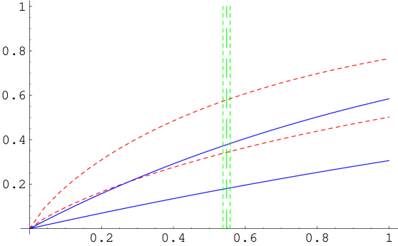
FIG. 1.: The time dependence of the von Neumann entropy (dashed lines), Eq.(40), and the loss of entanglement of formation $1-E$ (solid lines), given by Eq.(95), are plotted for the experimental mean value $\bar{\lambda}=1.84\cdot 10^{-12}\;\textrm{MeV}$ (lower curve) and the upper bound $\bar{\lambda}_{up}=4.34\cdot 10^{-12}\;\textrm{MeV}$ (upper curve), Eq.(28), of the decoherence parameter $\lambda$. The time $t$ is scaled versus the lifetime $\tau_{s}$ of the short lived kaon $K_{S}$: $t\to t/\tau_{s}$. The vertical lines represent the propagation time $t_{0}/\tau_{s}\approx 0.55$ of one kaon, including the experimental error bars, until it is measured by the absorber in the CPLEAR experiment.

For example, in case of the CPLEAR experiment, where one kaon propagates about 2 cm, which corresponds to a propagation time $t_{0}/\tau_{s}\approx 0.55$, until it is measured by an absorber, the loss of entanglement is about $18\%$ for the mean value and maximal $38\%$ for the upper bound of the decoherence parameter $\lambda$. These values, however, could diminish considerably in future experiments.

V Summary and conclusions

We have considered a simple model of decoherence of the entangled $K^{0}\bar{K}^{0}\;$state due to some environment, i.e. a master equation of Liouville - von Neumann type with an additional term $D[\rho]$. As generators of $D[\rho]$ causing the decoherence effect with strength $\lambda$ we choose the projectors to the eigenstates of the “effective mass” Hamiltonian and, for simplicity, $\mathcal{CP}\;$invariance is assumed. For this choice the time evolution for the components of $\rho$ decouples and only the off-diagonal elements are effected by our modification.

We apply the model to the data of the CPLEAR experiment, where we follow the philosophy that only the 2-particle state is affected by decoherence, whereas the 1-particle state evolves according to pure QM. We estimate in this way the strength $\lambda$ of the occurring decoherence, Eq.(28).

Moreover, we can relate the model to the case of a phenomenologically introduced decoherence parameter $\zeta$ and find a one-to-one correspondence, Eq.(37). However, the existing data are not yet sufficient to measure the time-dependence of $\zeta$ as predicted by our model, Eq.(36). So further measurements of the time-dependent asymmetry term, Eqs.(27), (35), would be of high interest in future experiments and will sharpen considerably the bounds of the parameters $\lambda$ and $\zeta$.

We can directly relate the decoherence of the $K^{0}\bar{K}^{0}\;$state to its loss of entanglement. In this connection we consider entanglement measures frequently discussed in the field of quantum information. We demonstrate that the initially pure singlet state of the entangled $K^{0}\bar{K}^{0}\;$becomes mixed for $0<t<\infty$ but remains entangled and achieves separability for $t\to\infty$ (see Proposition).

We find that entanglement loss in terms of the concurrence equals precisely the decoherence parameter $\zeta$, Eq.(96), and in terms of entanglement of formation the loss is very well approximated by $\frac{\zeta}{\ln 2}$ or $\frac{\lambda}{\ln 2}\cdot t$, Eq.(97), which is one of our main results. We can propose in this way how to measure experimentally the entanglement of the $K^{0}\bar{K}^{0}\;$system.

In Fig.1 we visualize both the loss of information given by the von Neumann entropy – which flows totally into the environment and not into the subsystems of the 2-particle system – and the loss of entanglement of formation. Inserting the mean value and upper bound of the parameter $\lambda$, which we have determined from the CPLEAR experiment, we obtain definite bounds for both the information- and entanglement loss of the propagating $K^{0}\bar{K}^{0}\;$system in dependence of the time. These values, however, could be improved considerably in future experiments.

VI Acknowledgement

The authors want to thank Časlav Brukner, Franz Embacher, Walter Grimus, Heide Narnhofer and Walter Thirring for helpful discussions. This research has been supported by the FWF Project No. P14143-PHY of the Austrian Science Foundation. The aid of the Austrian-Czech Republic Scientific Collaboration, project KONTAKT 2001-11, and of the EU project EURIDICE EEC-TMR program HPRN-CT-2002-00311 is acknowledged. Finally we would like to thank our referees for helpful comments.

REFERENCES

- [1] J. Six, Phys. Lett. B 114, 200 (1982).
- [2] F. Selleri, Lett. Nuovo Cim. 36, 521 (1983).
- [3] P. Privitera and F. Selleri, Phys. Lett. B 296, 261 (1992).
- [4] A. Bramon and G. Garbarino, Phys. Rev. Lett. 89, 160401 (2002).
- [5] G.C. Ghirardi, R. Grassi, and T. Weber, Quantum Mechanics Paradoxes at the -Factory, in Proc. of Workshop on Physics and Detectors for DANE, the Frascati -Factory, ed. G. Pancheri, Frascati, Italy, 1991.
- [6] F. Uchiyama, Phys. Lett. A 231, 295 (1997).
- [7] R.A. Bertlmann, W. Grimus, and B.C. Hiesmayr, Phys. Lett. A 289, 21 (2001).
- [8] R.A. Bertlmann and B.C. Hiesmayr, Phys. Rev. A 63, 062112 (2001).
- [9] A. Bramon and M. Nowakowski, Phys. Rev. Lett. 83, 1 (1999).
- [10] B. Ancochea, A. Bramon, and M. Nowakowski, Phys. Rev. D 60, 094008 (1999).
- [11] A. Bramon and G. Garbarino, Phys. Rev. Lett. 88, 403 (2002).
- [12] M. Genovese, C. Novero, and E. Predazzi, Phys. Lett. B 513, 401 (2001).
- [13] J. Ellis, J.S. Hagelin, D.V. Nanopoulos, and M. Srednicki, Nucl. Phys. B 241, 381 (1984).
- [14] J. Ellis, J.L. Lopez, N.E. Mavromatos, and D.V. Nanopoulos, Phys. Rev. D 53, 3846 (1996).
- [15] T. Banks, L. Susskind, and M.E. Peskin, Nucl. Phys. B 244, 125 (1984).
- [16] P. Huet and M.E. Peskin, Nucl. Phys. B 434, 3 (1995); ibid. B 488, 335 (1997).
- [17] R.A. Bertlmann, W. Grimus, and B.C. Hiesmayr, The EPR paradox in massive systems or about strange particles, in: Quantum [Un]speakables, R.A. Bertlmann and A. Zeilinger (eds.), p.163, Springer Verlag, Heidelberg, 2002; see also quant-ph/0106167.
- [18] F. Benatti and R. Floreanini, Phys. Lett. B 401 337 (1997).
- [19] A.A. Andrianov, J. Taron, and R. Tarrach, Phys. Lett. B 507, 200 (2001).
- [20] A. Datta and D. Home, Phys. Lett. A 119, 3 (1986).
- [21] R.A. Bertlmann and W. Grimus, Phys. Lett. B 392, 426 (1997).
- [22] G.V. Dass and K.V.L. Sarma, Eur. Phys. J. C 5, 283 (1998).
- [23] R.A. Bertlmann and W. Grimus, Phys. Rev. D 58, 034014 (1998).
- [24] A. Pompili and F. Selleri, Eur. Phys. J. C 14, 469 (2000).
- [25] E. Lisi, A. Marrone and D. Montanino, Phys. Rev. Lett. 85, 1166 (2000).
- [26] S. Hawking, Commun. Math. Phys. 87, 395 (1982).
- [27] G. ‘t Hooft, Class. Quant. Grav. 16, 3263 (1999).
- [28] G. ‘t Hooft, Determinism and Dissipation in Quantum Gravity, hep-th/0003005 .
- [29] G.C. Ghirardi, A. Rimini, and T. Weber, Phys. Rev. D 34, 470 (1986).
- [30] P. Pearle, Phys. Rev. A 39, 2277 (1989).
- [31] N. Gisin and I.C. Percival, J. Phys. A: Math. Gen. 25, 5677 (1992); ibid. 26, 2245 (1993).
- [32] R. Penrose, Gen. Rel. Grav. 28, 581 (1996); Phil. Trans. Roy. Soc. Lond. A 356, 1927 (1998).
- [33] B.C. Hiesmayr, The puzzling story of the neutral kaon system or what we can learn of entanglement, PhD thesis, University of Vienna, 2002.
- [34] J.S. Bell, Speakable and Unspeakable in Quantum Mechanics, Cambridge University Press, Cambridge, 1987.
- [35] CPLEAR Collaboration, A. Apostolakis et al., Phys. Lett. B 422, 339 (1998).
- [36] W.H. Furry, Phys. Rev. 49, 393 (1936).
- [37] R.A. Bertlmann and W. Grimus, Phys. Rev. D 64, 056004 (2001).
- [38] G. Lindblad, Comm. Math. Phys. 48, 119 (1976).
- [39] V. Gorini, A. Kossakowski, and E.C.G. Sudarshan, J. Math. Phys. 17, 821 (1976).
- [40] R.A. Bertlmann and W. Grimus, Phys. Lett. A 300, 107 (2002).
- [41] S.L. Adler, Phys. Rev. D 62, 117901 (2000).
- [42] F. Benatti and H. Narnhofer, Lett. Math. Phys. 15, 325 (1988).
- [43] R.A. Bertlmann, W. Grimus, and B.C. Hiesmayr, Phys. Rev. D 60, 114932 (1999).
- [44] B.C. Hiesmayr, Found. Phys. Lett. 14, 231 (2001).
- [45] P.H. Eberhard, Tests of quantum mechanics at a -factory, vol. 1. The Second DANE Physics Handbook; eds. L. Maiani, G. Pancheri and N. Paver (SIS-Publ. dei Laboratori Nazionali di Frascati), Frascati, Italy, 1995.
- [46] E. Schrödinger, Naturwissenschaften 23, 807 (1935); 23, 823 (1935). 23, 844 (1935).
- [47] B.C. Hiesmayr, The puzzling story of the -system or about quantum mechanical interference and Bell inequality in particle physics, Master’s thesis, University of Vienna, 1999.
- [48] BELLE-homepage, http://belle.kek.jp
- [49] G. Leder, talk given at the conference SUSY’02, Hamburg June 2002, http://wwwhephy.oeaw.ac.at/p3w/belle/leder_susy02.pdf
- [50] B.Aubert et al., BABAR Collaboration, Phys. Rev. D. 66, 032003 (2002).
- [51] BABAR-homepage, http://www.slac.stanford.edu/babar
- [52] H.-P. Breuer and F. Petruccione, The theory of open quantum systems, Oxford University Press, 2002.
- [53] E. Joos, Decoherence through interaction with the environment, in: Decoherence and the apperance of a classical world in quantum theory, D. Giulini et al. (eds.), p.35, Springer Verlag, Heidelberg, 1996.
- [54] O. Kübler and H.D. Zeh, Ann. Phys. (N.Y.) 76, 405 (1973).
- [55] E. Joos and H.D. Zeh, Z. Phys. B 59, 223 (1985).
- [56] W.H. Zurek, Physics Today 44, 36 (1991).
- [57] R. Alicki, Phys. Rev. A 65, 034104 (2002).
- [58] W. Thirring, Lehrbuch der Mathematischen Physik 4, Quantenmechanik großer Systeme, Springer Verlag, Wien, 1980.
- [59] R.A. Bertlmann, H. Narnhofer, and W. Thirring, Phys. Rev. A 66, 032319 (2002).
- [60] A. Peres, Phys. Rev. Lett. 77, 1413 (1996).
- [61] M. Horodecki, P. Horodecki, and R. Horodecki, Phys. Lett. A 223, 1 (1996).
- [62] M. Horodecki and P. Horodecki, Phys. Rev. A 59, 4206 (1999).
- [63] C.H. Bennett, D.P. DiVincenzo, J.A. Smolin, and W.K. Wootters, Phys. Rev. A 54, 3824 (1996).
- [64] S. Hill and W.K. Wootters, Phys. Rev. Lett. 78, 5022 (1997).
- [65] W.K. Wootters, Phys. Rev. Lett. 80, 2245 (1998).
- [66] W.K. Wootters, Quantum Information and Computation 1, 27 (2001).