Temporal build-up of electromagnetically induced transparency and absorption resonances in degenerate two-level transitions

Abstract

The temporal evolution of electromagnetically induced transparency (EIT) and absorption (EIA) coherence resonances in pump-probe spectroscopy of degenerate two-level atomic transition is studied for light intensities below saturation. Analytical expression for the transient absorption spectra are given for simple model systems and a model for the calculation of the time dependent response of realistic atomic transitions, where the Zeeman degeneracy is fully accounted for, is presented. EIT and EIA resonances have a similar (opposite sign) time dependent lineshape, however, the EIA evolution is slower and thus narrower lines are observed for long interaction time. Qualitative agreement with the theoretical predictions is obtained for the transient probe absorption on the ${}^{85}Rb$ $D_{2}$ line in an atomic beam experiment.

42.50.Gy, 42.50.Md, 32.80.Bx, 32.70.Jz.

I Introduction.

It is well known that the interaction of an atomic system with correlated optical waves can lead to quantum coherence in the atomic state. In turn, the atomic coherence dramatically modifies the interaction with the light [1]. A good example is provided by the effect of electromagnetically induced transparency (EIT) [2] where an absorbing medium can be rendered transparent to a probe field if it is simultaneously submitted to the action of a coupling field. EIT takes place when the two fields satisfy a two photon resonance condition between atomic levels. The corresponding (coherence) resonance for the probe absorption is called a “dark resonance” and is associated to the system being driven into a “dark state” i.e. a coherent superposition of atomic states uncoupled to the light field[3, 4].

In recent years, a new kind of coherence resonance was observed in which the atomic coherence results in an increase in the absorption of a probe field [5]. This phenomenon designated electromagnetically induced absorption (EIA), bears except for the sign of the resonance, several common features with EIT although it cannot be associated to the system being driven into a particular superposition of atomic states. EIA was first observed on a transition between two atomic levels with angular momentum degeneracy [5]. The degenerate two-level system (DTLS) was illuminated by  a resonant pump field and probed with a tunable probe field. It was clearly established that EIA is essentially a multilevel effect in the sense that it only takes place if both the lower and the upper atomic levels posses degeneracy. The condition for the occurrence of EIA in atomic transitions is $F_{e}>F_{g}>0$ where $F_{e}$ and $F_{g}$ are the total angular momenta of the excited and ground state respectively[5, 6, 7, 8]. The simplest model system for which EIA occurs is a four-level $N$ system theoretically investigated by Taichenachev et al [9]. The analysis of this system reveals that EIA is the consequence of the transfer of coherence from the upper to the lower atomic levels via spontaneous emission.

The transient properties of EIT has been explored by several authors in simple model systems [3]. In [10] the transient behavior of EIT in three level system when the pump field is suddenly switched on is considered and the onset of Rabi oscillations for saturating pump field intensities discussed. The occurrence of EIT for low intensities was analyzed in [11] for a closed three level $\Lambda$ system. It is established that EIT can take place even for very low intensities and that the characteristic time for the onset of the resonance is proportional to the square of the pumping field Rabi frequency divided by the excited state relaxation rate. Further investigation of EIT in $\Lambda$ systems involving the two hyperfine levels of alkaline atoms, can be found in [12] for different pump intensity regimes. In this work EIT in open $\Lambda$ systems is also considered and experimental data presented for $Na$. Coherence resonances in open three level systems were also theoretically and experimentally investigated using the Hanle/EIT scheme [13, 14, 15]. In this scheme, the frequencies of the optical fields are kept fixed and the atomic energy levels are scanned by a magnetic field. Analyzing in detail the case of the $F_{g}=1\rightarrow F_{e}=0$ transition, the authors conclude that the resonance width (in terms of the tunable magnetic field) decreases without limit as $t^{-1/2}$[15], $t$ being the interaction time. It is argued that this behavior is characteristic of open systems. Recently, the transient behavior of EIT resonances for sudden turn on and off of an intense pump field was experimentally investigated on a sample of magneto-optically cooled atoms [16, 17]. Large attention has also been paid to the temporal evolution of dark resonances when the light fields are switched on and off adiabatically[18, 19, 20]. In this case, reversible transfer of information from the light field to the atomic system can take place in connection with such effects as slow light propagation [21, 22] and light storage [23].

In this paper, we explore the evolution of the probe absorption spectrum in DTLS for atoms having spent a variable amount of time in presence of the pump and probe fields. Only field intensities below saturation are considered. Specifically, we focus on the analysis and comparison of the coherence resonances occurring on the cycling transitions of the $D_{2}$ ${}^{85}Rb$ lines when the atoms are illuminated by a pump and a probe field with tunable frequency difference and orthogonal linear polarizations. For the first transition studied, $5S_{1/2}\left(F=2\right)\rightarrow 5P_{3/2}\left(F^{\prime}=1\right)$ of ${}^{85}Rb$, EIT takes place while the second $5S_{1/2}\left(F=3\right)\rightarrow 5P_{3/2}\left(F^{\prime}=4\right)$ transition gives rise to EIA. The transient spectroscopy of the EIT resonances presented here is complementary of the observations in [13] for the $D_{1}$ line of $Na$ atoms under similar excitation conditions. The differences between the results in [13, 15] obtained with a Hanle setup and those presented here for pump-probe spectroscopy are stressed. To the best of our knowledge, the transient properties of EIA resonances are addressed in this work for the first time.

The paper is organized as follows. In order to introduce the main features of the dynamics of coherence resonances, the next section is devoted to the study of these resonances in simple model systems where EIT and EIA occur. In section III the coherence spectroscopy in realistic atomic systems (with angular momentum degeneracy) is considered and the transient evolution of EIT/EIA resonances obtained from numerical calculation. In section IV the experiments carried on a ${}^{85}Rb$ atomic beam are presented and discussed. Section V contains the conclusions.

II Model systems.

A EIT.

EIT can be conveniently analyzed in the $\Lambda$ system. Consider the level scheme presented in Fig. 1(i) where the two degenerate ground levels $a$ and $c$ (same energy) are coupled to the excited level $b$ (energy $\hbar\omega_{0}$, spontaneous emission decay rate $\Gamma$) by the pump field ${\cal E}_{1}(t)=2E_{1}\cos\left(\omega_{1}t\right)$  (with $E_{1}$ real) and the probe field ${\cal E}_{2}(t)=E_{2}\exp(-i\omega_{2}t)+cc$ respectively. The temporal evolution of the density matrix of the system is given by [11]:

$$\dot{\sigma}_{cc} = -i\Omega_{2}\sigma_{bc}+i\Omega_{2}^{\ast}\sigma_{cb}+\Gamma_{bc}\sigma_{bb}$$ (1)

$$\dot{\sigma}_{bb} = -i\Omega_{2}^{\ast}\sigma_{cb}+i\Omega_{2}\sigma_{bc}+-i\Omega_{1}\left(\sigma_{ab}-\sigma_{ba}\right)-\Gamma\sigma_{bb}$$ (2)

$$\dot{\sigma}_{aa} = -i\Omega_{1}\left(\sigma_{ba}-\sigma_{ab}\right)+\Gamma_{ba}\sigma_{bb}$$ (3)

$$\dot{\sigma}_{bc} = -\left[\frac{\Gamma}{2}+i\left(\omega_{0}-\omega_{2}\right)\right]\sigma_{bc}-i\Omega_{2}^{\ast}\left(\sigma_{cc}-\sigma_{bb}\right)-i\Omega_{1}\sigma_{ac}$$ (4)

$$\dot{\sigma}_{ab} = -\left[\frac{\Gamma}{2}-i\left(\omega_{0}-\omega_{1}\right)\right]\sigma_{ab}+i\Omega_{1}\left(\sigma_{aa}-\sigma_{bb}\right)+i\Omega_{2}\sigma_{ac}$$ (5)

$$\dot{\sigma}_{ac} = i\left(\omega_{2}-\omega_{1}\right)\sigma_{ac}-i\Omega_{1}\sigma_{bc}+i\Omega_{2}^{\ast}\sigma_{ab}$$ (6)

where the rotating wave approximation was used and the slow variables $\sigma_{ii}=\rho_{ii}$ ($i=a,b,c$), $\sigma_{ba}=e^{i\omega_{1}t}\rho_{ba}$, $\sigma_{bc}=e^{i\omega_{2}t}\rho_{bc}$, $\sigma_{ac}=e^{i(\omega_{2}-\omega_{1})t}\rho_{ac}$ were introduced. $\Gamma_{ba}$($\Gamma_{bc}$) is the radiative decay rate from $b$ to $a$($c$) ($\Gamma_{ba}+\Gamma_{bc}=\Gamma$), $2\Omega_{1}=\frac{2\mu_{ab}E_{1}}{\hbar}$  and $2\Omega_{2}=\frac{2\mu_{cb}E_{2}}{\hbar}$ are the Rabi frequencies for fields ${\cal E}_{1}$ and ${\cal E}_{2}$ respectively ($\mu_{ab}$ and $\mu_{cb}$ are the electric dipole matrix elements of the corresponding transitions).

For a weak probe we can seek a solution of Eq. 3 in the form:

$$\sigma(t)\approx\sigma^{0}(t)+\sigma^{1}(t)$$ (7)

where $\sigma^{n}(t)$ is of order $n$ in $\Omega_{2}$. For further simplification let us assume that the pump field is turned on at $t=-\infty$ while the probe field is switched on at $t=0$. With such assumptions, the zero order term of Eq. 7 is given, after substitution in Eqs. 3, by $\sigma_{aa}^{0}=\sigma_{bb}^{0}=\sigma_{ba}^{0}=\sigma_{bc}^{0}=\sigma_{ac}^{0}=0$, $\sigma_{cc}^{0}=1$.

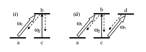
FIG. 1.: Model systems for EIT (i) and EIA (ii) coherence resonances. Dashed arrows indicate spontaneous emission decay channels.

The first order term in Eq. 7 obeys:

$$\dot{\sigma}_{bc}^{1} = -\left(\frac{\Gamma}{2}-i\delta\right)\sigma_{bc}^{1}-i\Omega_{2}^{\ast}\sigma_{cc}^{0}-i\Omega_{1}\sigma_{ac}^{1}$$ (8)

$$\dot{\sigma}_{ac}^{1} = -i\Omega_{1}\sigma_{bc}^{1}+i\delta\sigma_{ac}^{1}$$ (9)

where $\delta=\omega_{2}-\omega_{1}$ and we assumed for simplicity $\omega_{1}=\omega_{0}$ (exact resonance of the pumping field). The initial condition for the solution of Eqs. 8 is $\sigma^{1}(0)=0$. Introducing the optical pumping rate $\beta\equiv 2\frac{\Omega_{1}^{2}}{\Gamma}$, additional simplification of Eqs. 8 is possible when $\delta,\beta\ll\Gamma$. In this case, the optical coherence $\sigma_{bc}^{1}$ adiabatically follows the Raman coherence $\sigma_{ac}^{1}$. Taking $\dot{\sigma}_{bc}^{1}=0$ in Eq. 8 we get:

$$\sigma_{ac}^{1}\left(t\right) \simeq -\frac{2\Omega_{1}\Omega_{2}^{\ast}\sigma_{cc}^{0}}{\Gamma\left(\beta-i\delta\right)}\left\{1-\exp\left[-\left(\beta-i\delta\right)t\right]\right\}$$ (10)

$$\sigma_{bc}^{1}\left(t\right) \simeq -i\frac{\left[\Omega_{2}^{\ast}+\Omega_{1}\sigma_{ac}^{1}\left(t\right)\right]}{\left(\frac{\Gamma}{2}-i\delta\right)}$$ (11)

Consistently with the adiabatic following approximation, the temporal evolution of optical coherence is dependent on the transient behavior of the Raman coherence. $\sigma_{ac}^{1}\left(t\right)$ presents a damped oscillation at frequency $\delta$ with damping coefficient given by the optical pumping rate $\beta$.

At a given time, the power absorbed from the probe field is:

$$\alpha_{\Lambda}\left(t\right)\varpropto-\mathop{\rm Im}\left[\sigma_{bc}^{1}\left(t\right)\Omega_{2}\right]$$ (12)

and its stationary value:

$$\alpha_{\Lambda}^{ST}\varpropto\left|\Omega_{2}\right|^{2}\mathop{\rm Re}\left\{\frac{1}{\left(\frac{\Gamma}{2}-i\delta\right)}+\frac{2\Omega_{1}^{2}\sigma_{cc}^{0}}{\Gamma\left(\frac{\Gamma}{2}-i\delta\right)\left(\beta-i\delta\right)}\right\}$$ (13)

presents the characteristic EIT dip around $\delta=0$ with a linewidth (FWHM) of [3]:

$$\Delta_{\Lambda}\simeq 2\beta\equiv\frac{4\Omega_{1}^{2}}{\Gamma}$$ (14)

It is interesting in view of the comparison with the experiments described below to specify the non-linear absorption defined as the probe absorbed power in the presence of the pump field minus to the linear absorption (with no pump field):

$$\Delta\alpha_{\Lambda}\left(t\right) \varpropto \mathop{\rm Re}\left[\frac{\sigma_{ac}^{1}\left(t\right)\Omega_{1}\Omega_{2}}{\left(\frac{\Gamma}{2}-i\delta\right)}\right]$$ (15)

$$= -KF(\beta/\Gamma,\delta/\Gamma,\Gamma t)$$ (16)

where coefficient $K$ is proportional to the product of the intensities of the two fields and

$$F(x,y,\tau)\equiv\mathop{\rm Re}\left\{\frac{1-\exp\left[-\left(x-iy\right)\tau\right]}{\left(\frac{1}{2}-iy\right)\left(x-iy\right)}\right\}$$ (17)

The main features of the temporal and spectral behavior of the EIT resonance in the $\Lambda$ system result from the properties of the function $F(x,y,\tau)$ which is represented in Fig. 2. $F(x,y,0)=0$ as required by the initial condition. For $\tau\gg x^{-1},$ $F(x,y,\infty)$ represent a Lorentzian function of $y$ with FWHM given by $2x$. For $\tau\ll x^{-1}$, $F(x,y,\tau)$ is an even function of $y$ with a central peak of width $\sim 4\pi/\tau$ and oscillating wings with period $\sim 2\pi/\tau$. For fixed $x$ and $y$, $F(x,y,\tau)$ represent a damped oscillation with frequency $y/2\pi$ and damping rate $x$ [12].

FIG. 2.: Plot of the function $F(x,y,\tau)$ evaluated for $x=0.02$. a) $\tau$ dependence for fixed $y$. b) $y$ dependence for fixed $\tau$.

B EIA.

The simplest system presenting EIA is a four-level system in an $N$ configuration [Fig. 1(ii)]. EIA appears as the consequence of coherence transfer from the excited to the lower levels via spontaneous emission. This system was studied by Taichenachev et al [9] who calculate the analytical expression for the steady state probe absorption on the $c-b$ transition.

We explore the temporal evolution of the EIA resonance following the same procedure used for the $\Lambda$ system. The Bloch equations for the system are initially solved in the presence of the pump field alone and then a correction of the temporal evolution to first order in the probe field is determined. Again, for simplicity we assume that the system has reached its steady state under the presence of the pump field, when the probe field is turned on at $t=0$. Let the relative electric dipole matrix elements for the pairs of states $a-b$, $c-b$ and $c-d$ be $A$, $B$ and $1$ respectively with $\left|A\right|^{2}+\left|B\right|^{2}=1$. Introducing the slowly varying coefficients: $\sigma_{ii}=\rho_{ii}(i=a,b,c,d)$, $\sigma_{ba}=e^{i\omega_{1}t}\rho_{ba}$, $\sigma_{bc}=e^{i\omega_{2}t}\rho_{bc}$, $\sigma_{dc}=e^{i\omega_{1}t}\rho_{dc}$, $\sigma_{ca}=e^{i(\omega_{1}-\omega_{2})t}\rho_{ca}$, $\sigma_{bd}=e^{i(\omega_{2}-\omega_{1})t}\rho_{bd}$, $\sigma_{da}=e^{i(2\omega_{1}-\omega_{2})t}\rho_{da}$, we have in the rotating wave approximation:

$$\dot{\sigma}_{ac}^{1} = i\delta\sigma_{ac}^{1}-i\Omega_{1}A\sigma_{bc}^{1}+i\Omega_{1}\sigma_{ad}^{1}+\Gamma A\sigma_{bd}^{1}$$ (18)

$$\dot{\sigma}_{bc}^{1} = -i\Omega_{1}A\sigma_{ac}^{1}-\left(\frac{\Gamma}{2}-i\delta\right)\sigma_{bc}^{1}+i\Omega_{1}\sigma_{bd}^{1}-i\Omega_{2}^{\ast}\sigma_{cc}^{0}$$ (19)

$$\dot{\sigma}_{ad}^{1} = i\Omega_{1}\sigma_{ac}^{1}-\left(\frac{\Gamma}{2}-i\delta\right)\sigma_{ad}^{1}-i\Omega_{1}A\sigma_{bd}^{1}$$ (20)

$$\dot{\sigma}_{bd}^{1} = i\Omega_{1}\sigma_{bc}^{1}-i\Omega_{1}A\sigma_{ad}^{1}-\left(\Gamma-i\delta\right)\sigma_{bd}^{1}-i\Omega_{2}^{\ast}\sigma_{cd}^{0}$$ (21)

The Rabi frequency $2\Omega_{1}\left(2\Omega_{2}\right)$ of the pump(probe) field refers to the $c-d$ ($c-b$) transition and $\sigma_{cc}^{0}$ and $\sigma_{cd}^{0}$ are the stationary non-zero matrix elements resulting from the interaction with the pump field alone.

As for the $\Lambda$ system, Eqs. 19 can be solved assuming that $\sigma_{bc}^{1}$, $\sigma_{ad}^{1}$ and $\sigma_{bd}^{1}$ adiabatically follow the Raman coherence $\sigma_{ac}^{1}$. Thus, neglecting $\dot{\sigma}_{bc}^{1}$, $\dot{\sigma}_{ad}^{1}$ and $\dot{\sigma}_{bd}^{1}$ in Eqs. 19, after some calculation we get to the lowest order in $\delta$ and $\Omega_{1}^{2}/\Gamma$:

$$\sigma_{ac}^{1}\left(t\right) \simeq -\frac{2A\Omega_{1}\Omega_{2}^{\ast}}{\Gamma\left(\beta^{\prime}-i\delta\right)}\left\{1-\exp\left[-\left(\beta^{\prime}-i\delta\right)t\right]\right\}$$ (22)

$$\beta^{\prime} = \frac{2\Omega_{1}^{2}}{\Gamma}\left(1-\left|A\right|^{2}\right)=\beta\left(1-\left|A\right|^{2}\right)$$ (23)

and

$$\sigma_{bc}^{1}\left(t\right)\simeq\frac{-i\Omega_{2}^{\ast}}{\frac{\Gamma}{2}-i\delta}(1-4\frac{\left|\Omega_{1}\right|^{2}}{\Gamma^{2}}$$ (24)

$$+2A^{2}\frac{\left|\Omega_{1}\right|^{2}}{\Gamma\left(\beta^{\prime}-i\delta\right)}\left\{1-\exp\left[-\left(\beta^{\prime}-i\delta\right)t\right]\right\})$$ (25)

Using Eq. 12, the steady state probe absorbed power is [9]:

$$\alpha_{N}^{ST}\varpropto\left|\Omega_{2}\right|^{2}\mathop{\rm Re}\left\{\frac{1}{\frac{\Gamma}{2}-i\delta}\left[1-4\frac{\left|\Omega_{1}\right|^{2}}{\Gamma^{2}}+2A^{2}\frac{\left|\Omega_{1}\right|^{2}}{\Gamma\left(\beta^{\prime}-i\delta\right)}\right]\right\}$$ (26)

and the time dependent non-linear absorption:

$$\Delta\alpha_{N}\left(t\right)=-\frac{K^{\prime}}{\left[\left(\frac{\Gamma}{2}\right)^{2}+\delta^{2}\right]}+K^{\prime}\frac{A^{2}}{\Gamma^{2}}F(\beta^{\prime}/\Gamma,\delta/\Gamma,\Gamma t)$$ (27)

with $K^{\prime}$ proportional to the product of the two fields intensities. The first term in Eq. 27 correspond to a broad (linewidth $\sim\Gamma$) reduction in the absorption due to the saturation of the $c-d$ transition by the pump field. The second term represents the EIA resonance. It has a similar spectral and temporal dependence than the EIT resonance (see Eq. 15) except for the sign inversion. Notice however the reduction by the “narrowing factor” $1-\left|A\right|^{2}$ (see Eq. 23) of the damping rate (and stationary spectral width) of the EIA resonance compared to the EIT resonance in the $\Lambda$ system. As a consequence, EIA is expected to be considerably slower in its evolution than EIT for optical transition with comparable electric dipole matrix elements (comparable Clebsh-Gordan coefficients for DTLS).

III Realistic atomic systems.

The previous analysis apply to ideal $\Lambda$ and $N$  level configurations. Actual experiments are frequently carried on DTLS where, depending on their polarization, the pump and probe fields couple different pairs of Zeeman sublevels resulting in a large variety of (generally more complex) level schemes.

Before considering in more detail DTLS, let us briefly mention the case of a pure two level transition driven by a pump and a probe fields of frequencies $\omega_{1}$ and $\omega_{2}$ respectively. Unlike the $\Lambda$ and $N$ systems where each field drives different transitions, here the same transition is driven by both fields. This results in a pulsation of the populations of the lower and upper levels at the beat frequency $\delta\equiv\omega_{2}-\omega_{1}$. As a consequence, the atomic coherence between the ground and excited state posses several frequency components ($\omega_{1},\omega_{2},2\omega_{1}-\omega_{2}$) giving rise to a modulation of the probe absorption at the harmonics of the beat frequency [24].

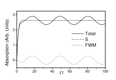
FIG. 3.: Transient evolution of the probe absorption of a pure two-level system. $\Omega_{1}=0.08\ \Gamma$, $\delta=0.1\ \Gamma$. S: synchronous contribution, FWM: four-wave mixing contribution (see text).

A similar behavior occur for DTLS driven by two fields. Except for the simplest combinations of pump and probe polarizations (like $\sigma^{+},\ \sigma^{-}$), the excitation of a DTLS with two optical fields result in population pulsation and the presence of a new frequency component $(2\omega_{1}-\omega_{2})$ for the atomic coherence between ground and excited state (optical coherence). We shall call this component “FWM component” since it is responsible for the emission of a new field at frequency $2\omega_{1}-\omega_{2}$ via four-wave mixing [7]. The FWM component of the atomic optical coherence results in a modulated contribution to the probe absorption with frequency $2\delta$. In contrast, we shall call “synchronous” (S) the contribution to the probe absorption of the atomic optical coherence oscillating at frequency $\omega_{2}$. Fig. 3 illustrate the temporal behavior of the probe absorption (for a pure two level system) showing the S and FWM contributions.

Two features characterize the oscillation due to the FWM contribution: $i)$ It is a permanent oscillation not to be mistaken with the damped oscillation at frequency $\delta$ that can be present in the S contribution (see Eqs. 15 and 27). $ii)$ The phase of the oscillation depend on the relative phase between the pump and probe fields [25]. Both features are of crucial importance in the experiments. In the experiment described below, only the S contribution to the probe absorption is observed. The oscillating character of FWM results in the averaging to zero of this contribution when $\delta\gg T^{-1}$ ($T$ is the temporal resolution in the experiment). Even for $\delta\lesssim T^{-1}$ the FWM contribution is washed out due to the occurrence of random (and rapid) fluctuations of the phase difference between the pump and probe field (due to mechanical vibrations in the setup). The observation of the FWM contribution should require a careful interferometric control of the phase difference between the two fields and temporal resolution better than $\delta^{-1}$.

We will next present a theoretical model allowing the calculation, to first order in the probe field, of the transient probe absorption for DTLS with arbitrary choices of the ground and excited levels angular momenta and polarizations of the pump and probe fields. The model is a direct application to the time domain of the treatment previously used for the study of the steady state spectral characteristics of coherence resonances [7]. It allows the identification of the S and FWM contributions in the probe absorption.

We consider two degenerate levels: a ground level $g$ of total angular momentum $F_{g}$ and energy $\hbar\omega_{g}$ and an excited state $e$ of angular momentum $F_{e}$ and energy $\hbar\omega_{e}$. The radiative relaxation coefficient of level $e$ is $\Gamma$. We restrict ourselves to closed transitions. Extension of the model to open transitions is straightforward [7].

The atoms are initially in the ground state described by an isotropic density matrix $\rho_{0}$. They are submitted to a magnetic field $B$ along the quantization axis and to two classical optical fields:

$\displaystyle{\cal E}_{j}(t)=E_{j}\hat{e}_{j}e^{i\omega_{j}t}+E_{j}^{\ast}\hat{e}_{j}^{\ast}e^{-i\omega_{j}t},\ (j=1,2)$
$\widehat{e}_{j}$ are complex polarization vectors. The Hamiltonian of the system is:

$$H(t)=H_{0}+V_{1}\left(t\right)+V_{2}\left(t\right)$$ (28)

with:

$$H_{0} = H_{A}+H_{B}$$ (29)

$$H_{A} = \hbar\left(P_{e}\omega_{e}+P_{g}\omega_{g}\right)$$ (30)

$$H_{B} = -\mu_{B}F_{z}\left(g_{g}P_{g}+g_{e}P_{e}\right)B$$ (31)

$$V_{j} = E_{j}\hat{e}_{j}\cdot\vec{D}_{ge}e^{i\omega_{j}t}+E_{j}^{\ast}\hat{e}_{j}^{\ast}\cdot\vec{D}_{eg}e^{-i\omega_{j}t}$$ (32)

here $P_{g}$ and $P_{e}$ are the projectors on the ground and excited manifolds respectively. $H_{B}$ is the Zeeman Hamiltonian, $g_{g}$ and $g_{e}$ are the gyromagnetic factors of the ground and excited levels respectively, $\mu_{B}$ is the Bohr magnetron and $\hbar F_{z}$ the projection of the total angular momentum along the quantization axis. $\vec{D}_{ge}=\vec{D}_{eg}^{\dagger}=P_{g}\vec{D}P_{e}$ is the lowering part of the atomic dipole operator (we assume that $P_{g}\vec{D}P_{g}=P_{e}\vec{D}P_{e}=0$). In Eq. 32 the usual rotating wave approximation is used.

The temporal evolution of the atomic density matrix $\rho$ is governed by the master equation:

$$\frac{\partial\rho}{\partial t} = -\frac{i}{\hbar}\left[H,\rho\right]-\frac{\Gamma}{2}\left\{P_{e,}\rho\right\}$$ (34)

$$+\Gamma\sum_{q=-1,0,1}Q_{ge}^{q}\rho Q_{eg}^{q}$$

where $Q_{ge}^{q}=Q_{eg}^{q\dagger}\ \left(q=-1,0,1\right)$ are the standard components of the dimensionless operator:

$$\vec{Q}_{ge}=\sqrt{2F_{e}+1}\frac{\vec{D}_{ge}}{\left\langle g\|\vec{D}\|e\right\rangle}$$ (35)

$\left\langle g\|\vec{D}\|e\right\rangle$ is the reduced matrix element of the electric dipole operator.

In order to find the response of the system to the two fields, we first consider the effect of the pump field ${\cal E}_{1}$ and next we calculate the effect of the probe field ${\cal E}_{2}$ to first order.

It is convenient to introduce the slowly varying matrix $\sigma_{0}$ given by:

$$\sigma^{0} = \sigma_{gg}^{0}+\sigma_{ee}^{0}+\sigma_{ge}^{0}+\sigma_{eg}^{0}$$ (36)

$$\sigma_{gg}^{0} = P_{g}\rho P_{g}$$ (37)

$$\sigma_{ee}^{0} = P_{e}\rho P_{e}$$ (38)

$$\sigma_{ge}^{0} = P_{g}\rho P_{e}e^{-i\omega_{1}t}$$ (39)

$$\sigma_{eg}^{0} = P_{e}\rho P_{g}e^{i\omega_{1}t}$$ (40)

after substitution into Eq. 34 (with $V_{2}=0$) one has for $\sigma^{0}(t)$ the equation:

$$\frac{d\sigma^{0}}{dt} = -\frac{i}{\hbar}\left[H_{0}+\bar{V}_{1}-\hbar\omega_{1}P_{e},\sigma^{0}\right]-\frac{\Gamma}{2}\left\{P_{e},\sigma^{0}\right\}$$ (42)

$$+\Gamma\sum_{q=-1,0,1}Q_{ge}^{q}\sigma^{0}Q_{eg}^{q}$$

with:

$$\bar{V}_{1}=E_{1}\hat{e}_{1}\cdot\vec{D}_{ge}+E_{1}^{\ast}\hat{e}_{1}^{\ast}\cdot\vec{D}_{eg}$$ (43)

and the initial condition $\sigma^{0}(0)=\rho_{0}$.

To include the effect (to first order) of the probe field on the atom+pump system, we seek a solution of Eq. 34 under the form:

$$\rho_{gg}(t) = P_{g}\rho\left(t\right)P_{g}=\sigma_{gg}^{0}+\sigma_{gg}^{+}e^{i\delta t}+\sigma_{gg}^{-}e^{-i\delta t}$$ (44)

$$\rho_{ee}(t) = P_{e}\rho\left(t\right)P_{e}=\sigma_{ee}^{0}+\sigma_{ee}^{+}e^{i\delta t}+\sigma_{ee}^{-}e^{-i\delta t}$$ (45)

$$\rho_{ge}(t) = P_{g}\rho\left(t\right)P_{e}=e^{i\omega_{1}t}\left(\sigma_{ge}^{0}+\sigma_{ge}^{+}e^{i\delta t}+\sigma_{ge}^{-}e^{-i\delta t}\right)$$ (46)

$$\rho_{eg}(t) = P_{e}\rho\left(t\right)P_{g}=e^{-i\omega_{1}t}\left(\sigma_{eg}^{0}+\sigma_{eg}^{+}e^{i\delta t}+\sigma_{eg}^{-}e^{-i\delta t}\right)$$ (47)

with $\delta=\omega_{2}-\omega_{1}$.

Introducing the non Hermitian matrix:

$$\sigma=\left(\begin{array}[]{ll}\sigma_{gg}^{+}&\sigma_{ge}^{+}\\ \sigma_{eg}^{+}&\sigma_{ee}^{+}\end{array}\right)$$ (48)

After substitution into Eq. 34 and keeping only terms to first order in $E_{2}$ one has:

$$\frac{d\sigma}{dt}=-\frac{i}{\hbar}\left[H_{0}+\bar{V}_{1}-\hbar\omega_{1}P_{e},\sigma\right]-i\delta\sigma-\frac{\Gamma}{2}\left\{P_{e},\sigma\right\}$$ (49)

$$+\Gamma\sum_{q=-1,0,1}Q_{ge}^{q}\sigma Q_{eg}^{q}-i\left[\frac{\Theta_{2}}{2},\sigma^{0}(t)\right]$$ (50)

where we have introduced $\Theta_{2}\equiv(2\vec{E}_{2}\cdot\vec{D}_{ge})/\hbar$. Here the initial condition is: $\sigma(0)=0$.

If the pump field is turned on long before the probe field, then $\sigma^{0}(t)$ is time independent and Eq. 50 corresponds to a linear differential equation with constant coefficients. Even if a different initial condition for the pump field is chosen, the numerical solution of Eq. 50 can be easily implemented.

The density matrix $\sigma\left(t\right)$ contains all the relevant information concerning the response to the probe field to first order. The information concerning the optical atomic polarization oscillating at the probe frequency (S contribution) is determined by the sub-matrix $\sigma_{ge}^{+}$ (see Eqs. 46) while FWM contribution depends on $\sigma_{eg}^{+}$.

The probe absorption coefficient due to the S contribution to the atomic optical polarization is given by:

$$\alpha_{S}\varpropto\widehat{e}_{2}\cdot Imag\left[Tr\left(\sigma_{ge}^{+}\vec{D}_{eg}\right)\right]$$ (51)

and the absorption dependent on the FWM contribution:

$$\alpha_{FWM}\varpropto-\widehat{e}_{2}\cdot Imag\left[Tr\left(\sigma_{eg}^{+}\vec{D}_{ge}\right)e^{i2\delta t}\right]$$ (52)

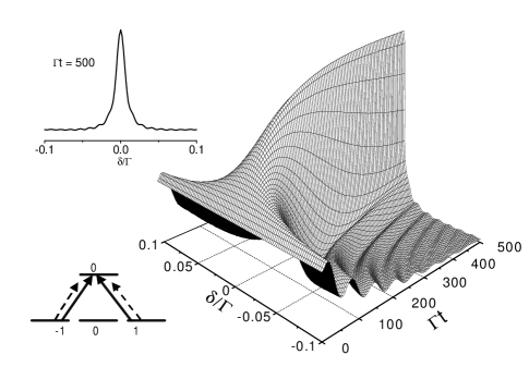
FIG. 4.: Calculated temporal and spectral dependence of the nonlinear probe absorption for a closed $F_{g}=1\rightarrow F_{e}=0$ transition. The pump and probe polarizations are linear and perpendicular, $\Omega_{1}=0.2\ \Gamma$. Both fields are turned on at $t=0$. The vertical axis (Arb. units) indicates increasing transparency.

The predictions of the previous model are illustrated in Figs. 4 and 5 showing the time dependence of the absorption spectra arising from the S contribution for two different transitions with $B=0$. Only the non-linear probe absorption (total absorption minus linear absorption) is plotted. The pump and probe fields have linear and perpendicular polarizations. The calculations were carried in both cases assuming that the atoms are initially in the ground state (no coherence and uniform population distribution among Zeeman sublevels) and that the pump and the probe fields are simultaneously turned on at $t=0$ (as suggested by the experiments described below). Fig. 4 corresponds to an $F_{g}=1\rightarrow F_{e}=0$ transition for which EIT occurs. The vertical axis indicate increasing transparency. The constant level at $t=0$ correspond to the linear absorption for unpumped atoms. Notice the increase in the average absorption level for nonzero $\delta$ corresponding to the ground state alignment produced by the pump field. As in the simple models previously analyzed, the absorption present coherent oscillations at the Raman detuning $\delta$. At short times, the lineshape is given by a central peak of width inversely proportional to $t$, with oscillating wings. At longer times the spectrum approaches a Lorentzian shape with a width proportional to the intensity of the pumping field [12]. The results presented in Fig. 4 correspond to the same atomic system analyzed in [15]. The system is equivalent to an open $\Lambda$ system since the atom can decay from the excited state into the $m_{g}=0$ ground state Zeeman sublevel not coupled by the light. In contrast to what occurs in the same system for the Hanle type experiment, the width of the EIT resonance, approaches a finite linewidth at long times determined by the intensity of the pump field. Such behavior is common to coherence resonances in closed [10] and open [12] $\Lambda$ systems observed through pump-probe spectroscopy. The fact that no qualitative difference in the time dependence of the resonance width is observed between closed and open transitions is a consequence of the assumption that the probe field is weak and does not modify the Zeeman sublevels populations. Fig. 5 corresponds to the EIA type transition $F_{g}=1\rightarrow F_{e}=2$. The vertical axis indicate increasing absorption. The nonlinear probe absorption was calculated for the same parameters, aside from the choice of the transition, than in Fig. 4. Observe the noticeable slowing of the EIA evolution in comparison with EIT. For the time interval presented in Fig. 5 (see inset) the nonlinear absorption spectrum is still far from reaching the asymptotic Lorentzian shape. This result suggest that the EIA slowing (and consequently narrowing) introduced above via the simple $N$ system is a general feature. We have checked numerically that the characteristic evolution time of the EIA resonances is an increasing function of the total angular momentum of the atomic levels involved.

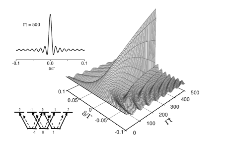
FIG. 5.: Calculated temporal and spectral dependence of the nonlinear probe absorption for a closed $F_{g}=1\rightarrow F_{e}=2$ transition. The pump and probe polarizations are linear and perpendicular, $\Omega_{1}=0.2\ \Gamma$. Both fields are turned on at $t=0$. The vertical axis (Arb. units) indicates increasing absorption.

We have chosen to illustrate the preceding analysis, the transitions $F_{g}=1\rightarrow F_{e}=0$ and $F_{g}=1\rightarrow F_{e}=2$ which are the simplest (with integer angular momenta) to present EIT and EIA. We have checked that similar conclusions stand for other choices of the angular momenta and in particular for the $F_{g}=2\rightarrow F_{e}=1$ and $F_{g}=3\rightarrow F_{e}=4$ transitions occurring in the $D_{2}$ line of ${}^{85}Rb$.

Finally, let us briefly comment on the effect of a nonzero magnetic field. In view of the experimental conditions presented below, we focus on moderate magnetic fields and restrict the range of variation of $\delta$ in order to verify $\left|\delta\right|<g_{g}\mu_{B}B<\Gamma$. In consequence, only the coherence resonance around $\delta=0$ ($\Delta m_{g}=0$) is considered. We have checked that under such assumptions, the main characteristics discussed above for the transient spectral behavior of the coherence resonances are generally preserved [26]. However, some differences are observed: An additional frequency component of the nonlinear absorption oscillating at the Larmor frequency $2g_{g}\mu_{B}B$ appears and there are also quantitative variations on the resonance peak amplitude and on the average absorption outside the peak. A detailed study of the influence of the magnetic field on the coherence resonances dynamics is beyond the scope of this paper.

IV Experiment.

We have studied the transient spectral behavior of coherence resonances arising on the $D_{2}$ transitions of ${}^{85}Rb$ atoms in an atomic beam. The experimental scheme is represented in Fig. 6. The atomic beam has a $Rb$ reservoir chamber heated to $180{{}^{o}}C$. The atoms exit the heating chamber through a $1\ cm$ diameter, $6\ mm$ long cylindrical nozzle formed by an array of parallel tubes of $0.5\ mm$ internal diameter. The collimation of the atomic beam is achieved with a rectangular slit ($1\ mm\times 10\ mm$) situated $25\ cm$ downstream. The estimated atomic flux after the collimation slit was $2\times 10^{15}$ $atoms/s$.

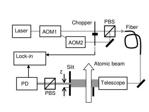
FIG. 6.: Experimental setup. PBS: polarizing beam splitter. AOM: acousto-optic modulator. PD: photodiode.

The optical beams are obtained by an injected diode laser ($\sim 1\ MHz$ linewidth). Using two consecutive acousto-optic modulators (AOM), one of which is driven by a tunable RF source, mutually coherent pump and probe beams are obtained [5] with variable frequency offset. The two optical fields have orthogonal linear polarizations. They are combined in a polarizing beam splitter and sent though a $50\ cm$ long single-mode fiber (that preserves polarization) for perfect overlap. After the fiber, the beam is expanded with a telescope. Only the central part of the expanded beam where the intensity is approximately constant (less than $10\%$ variation) is used to illuminate the atomic sample.

The atomic beam is intersected at right angle by the light beam. The shadow of the rectilinear edge of an opaque screen introduces a sudden transition between obscurity and light for the incoming atoms. Using a movable slit of width $\Delta z=0.5\ mm$ wide, the transmitted light is collected at different positions after the entrance of the atoms in the illuminated region. The probe absorption spectra are recorded as a function of the frequency difference $\delta$ between the probe and pump fields for different values of the slit position $z$. Each spectrum corresponds to atoms having interacted with the light during an average interval $t=z/\bar{v}$ where $\bar{v}$ is the mean velocity in the atomic beam. After the slit, the pump field is blocked with a linear polarizer. The transmitted probe light is detected with a photodiode.

A small magnetic field ($\sim 2\ G$), oriented in the direction of the light propagation, was applied to the interaction region to eliminate the broadening of the coherence resonances arising from magnetic field inhomogeneities. Due to this field, only $\Delta m_{g}=0$ resonances are observed which are insensitive to the magnetic field strength [5]. The magnetic field introduces a rapid oscillation of the probe absorption (at the Larmor frequency) with a period of approximately $0.5\ \mu s.$ Since the temporal resolution in the experiment is $\Delta t\simeq\Delta z/\bar{v}\approx 1.3\ \mu s$ such oscillation is not observed.

In order to improve sensitivity and have direct access to the nonlinear absorption, a two-frequencies modulation technique was used. The pump and probe fields are mechanically chopped at frequencies $f_{1}$ and $f_{2}$ respectively and the photodiode current is analyzed with a lock-in amplifier at the sum frequency $f_{1}+f_{2}$ ($\sim 300\ Hz$).

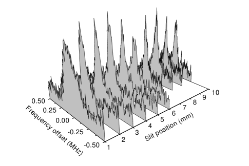
FIG. 7.: Experimental nonlinear probe absorption spectra at different positions of the movable slit for the $5S_{1/2}\left(F=2\right)\rightarrow 5P_{3/2}\left(F^{\prime}=1\right)\$transition of $\ {}^{85}Rb$. The vertical axis (Arb. units) indicates decreasing absorption.

The temporal and spectral evolution of the probe absorption for the two closed transitions of the $D_{2}$ line of ${}^{85}Rb$ are shown in Figs. 7 and 8 recorded for a pump field intensity $I_{1}=0.1\ mW/cm^{2}$. Fig. 7 correspond to the nonlinear probe absorption on the $5S_{1/2}\left(F=2\right)\rightarrow 5P_{3/2}\left(F^{\prime}=1\right)$ transition for which EIT occurs. The vertical axis is linear and corresponds to increasing transparency. A noticeable the narrowing of the spectra occurs for the two initial values of the slit position $z$ and no further narrowing of the spectra is observed for larger values of $z$ (the lineshape is approximately Lorentzian for all $z$’s). This fact, together with the rapid increase of the peak transparency indicate that the atoms attain their steady state after $\sim 1\ mm$ flight inside the light beam. For longer interaction times the linewidth remains unchanged and is determined by the intensity of the pump field.

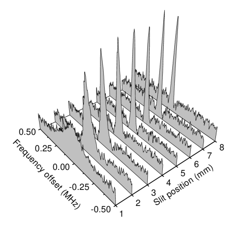
FIG. 8.: Experimental nonlinear probe absorption spectra at different positions of the movable slit for the $5S_{1/2}\left(F=3\right)\rightarrow 5P_{3/2}\left(F^{\prime}=4\right)\$transition of $\ {}^{85}Rb$. The vertical axis (Arb. units) indicate increasing absorption.

Fig. 8  corresponds to the nonlinear probe absorption on the $5S_{1/2}\left(F=3\right)\rightarrow 5P_{3/2}\left(F^{\prime}=4\right)$ transition (EIA resonance) recorded for the same pump intensity. The vertical axis corresponds to increasing absorption. A much slower evolution is observed in comparison with the EIT resonance. Notice the continuous narrowing of the coherence resonance for increasing values of $z$ over all the range shown and the relatively slow increase of the absorption peak for $\delta=0$ as a function of $z$. Even for the largest $z$, the lineshape is clearly not Lorentzian. It resembles the characteristic shape of the function $F(x,y,\tau)$ for $\tau\lesssim x^{-1}$  and is in good correspondence with the calculated lineshape (see the inset in Fig. 5). The narrowest peak observed for EIA  has approximately $20\ kHz$ FWHM. Fig. 9 illustrate the oscillatory behavior of the absorption as a function of $z$ for $\delta/2\pi=100\ kHz$. The spatial frequency of a sine wave fitted to the experimental data (solid line in Fig. 9) is consistent with a mean atomic velocity $\bar{v}\simeq 4.3\pm 0.4\times 10^{2}\ m/s$ in agreement with the value estimated from the $Rb$ reservoir temperature. One concludes that in the conditions of Fig. 5, the steady state is not reached within the observation range. Considering that the line strength of the $5S_{1/2}\left(F=3\right)\rightarrow 5P_{3/2}\left(F^{\prime}=4\right)$ transition is larger by a factor of $3$ than that of the $5S_{1/2}\left(F=2\right)\rightarrow 5P_{3/2}\left(F^{\prime}=1\right)$ transition, one has to conclude that the slower EIA evolution (compared to EIT) is not due to a smaller pump field Rabi frequency. Instead the observation suggest that it is due to a “narrowing factor” as the one introduced in Eq 23.

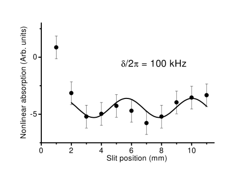
FIG. 9.: Time dependence of the nonlinear probe absorption for the $5S_{1/2}\left(F=3\right)\rightarrow 5P_{3/2}\left(F^{\prime}=4\right)\$transition of $\ {}^{85}Rb$ for $\delta/2\pi=100\ kHz$. Solid line: sine wave fit.

V Conclusions.

We have examined the temporal evolution of the spectral response of degenerate two level system observed using pump probe spectroscopy. The main features of the transient spectra arise from the consideration of simple models appropriate to the study of EIA and EIT. These models predict a similar evolution of the transient response in both cases although EIA appear to be considerably slower due to the narrowing factor identified in Eq. 23. A convenient model for the calculation of the transient response of DTLS was presented. It allows the identification and separation of the synchronous and the oscillating FWM contributions to the probe absorption. The numerically calculated transient evolutions of the EIT and EIA resonances occurring for $F_{g}=1\rightarrow F_{e}=0$ and $F_{g}=1\rightarrow F_{e}=2$ transitions respectively, are in good qualitative agreement with the simple models previously discussed. In both cases, the resonance width decreases as the inverse of the interaction time and approaches an asymptotic value determined by the pump field intensity. Under the same excitation conditions the EIA resonances are slower (and consequently narrower). Good qualitative agreement with the predicted transient spectral behavior was obtained for the EIT and EIA transitions on the $D_{2}$ line of ${}^{85}Rb$.

VI Acknowledgments.

The authors acknowledge stimulating discussions with D. Bloch. This work was supported by the Uruguayan agencies: CONICYT, CSIC and PEDECIBA and by ECOS (France).

REFERENCES

- [1] For a general overview of coherent processes see M.O. Scully and M.S. Zubairy, Quantum Optics, Cambridge University Press, Cambridge (1997) and references therein.
- [2] see S. E. Harris, Physics Today, 50(7) 36 (1997) and references therein.
- [3] B.D. Agap’ev, M.D. Gornyï and B.G. Matisov, Physics-Uspekhi 36, 763 (1993) [Usp. Fiz. Nauk 163, 1 (1993)].
- [4] E.Arimondo, Coherent population trapping, Progress in Optics XXXV, 257 (1996) and references therein.
- [5] A.M. Akulshin, S. Barreiro and A. Lezama, Phys. Rev. A 57, 2996 (1998).
- [6] A. Lezama, S. Barreiro and A.M. Akulshin, Phys. Rev. A. 59, 4732 (1999).
- [7] A. Lezama, S. Barreiro,. A. Lipsich and A.M. Akulshin, Phys. Rev. A 61, 013801 (2000).
- [8] Y. Dancheva, G. Alzetta, S. Cartaleva, M. Taslakov and Ch. Andreeva, Opt. Commun. 178, 103 (2000).
- [9] A.V. Taichenachev, A.M. Tumaikin and V.I. Yudin, Phys. Rev. A 61, 011802 (2000).
- [10] Yong-qing Li and Min Xiao, Opt. Lett. 20, 1489 (1995).
- [11] I.V. Jyotsna and G.S. Agarwal, Phys. Rev. A 52, 3147 (1995).
- [12] E.A. Korsunsky, W. Maichen and L. Windholz, Phys. Rev. A 56, 3908 (1997).
- [13] F. Renzoni, W. Maichen, L. Windholz and E. Arimondo, Phys. Rev. A 55, 3710 (1997).
- [14] F. Renzoni and E. Arimondo, Phys. Rev. A 58, 4717 (1998).
- [15] F. Renzoni, A. Lindner and E. Arimondo, Phys. Rev. A 60, 450 (1999).
- [16] H.X. Chen, A.V. Durrant, J.P. Marangos and J.A. Vaccaro, Phys. Rev. A, 58, 1545 (1998).
- [17] A.D. Greentree, T.B. Smith, S.R. de Echaniz, AV. Durrant, J. P. Marangos, D.M. Segal and J.A. Vaccaro, Phys. Rev. A 65, 053802 (2002).
- [18] J.R. Kuklinsky, U. Gaubatz, F.T. Hioe and K. Bergmann, Phys. Rev. A, 40, 6741 (1989).
- [19] M. Fleischhauer, S.F. Yelin and M.D. Lukin, Optics Commun. 179, 395 (2000).
- [20] M. Fleischhauer and M.D. Lukin, Phys. Rev. Lett. 84, 5094 (2000).
- [21] L.V. Hau, S.E. Harris, Z. Dutton and C.H. Behroozi, Nature 397, 594 (1999).
- [22] M.M. Kash et al, Phys. Rev. Lett. 82, 5229 (1999).
- [23] D.F. Phillips, A. Fleischhauer, A. Mair, R.L. Walsworth and M.D. Lukin, Phys. Rev. Lett. 86, 783 (2001).
- [24] V.S. Letokhov and V.P. Chebotayev, Nonlinear Laser Spectroscopy, Springer Series in Optical Sciences Vol 4 (Springer Verlag, Berlin, 1977).
- [25] E.A. Korsunsky, N. Leinfellner, A. Huss, S. Baluschev, and L. Windholz, Phys. Rev. A 59, 2302 (1999).
- [26] The transition is a special case since for nonzero magnetic field the pump will eventually drive all the population into the sink state not coupled by the probe.