Binary Decision Diagrams are
a Subset of Bayesian Nets

Abstract

The goal of this brief pedagogical article is to show that Binary Decision Diagrams are a special kind of Bayesian Net. This observation is obvious to workers in these two fields, but it might not be too obvious to others.

The goal of this brief pedagogical article is to show that Binary Decision Diagrams[1][2] are a special kind of Bayesian Net[3]. This observation is obvious to workers in these two fields, but it might not be too obvious to others.

Let $Bool=\{0,1\}$ where $0=false$ and $1=true$. For any integer $n$, functions $f:Bool^{n}\rightarrow Bool$ are called Boolean expressions. Suppose $x,y\in Bool$. As is conventional, we will use $x\vee y$ (resp., $x\wedge y$) to denote the Boolean function of $x$ and $y$ that evaluates to true if and only if $x$ OR $y$ (resp., $x$ AND $y$) is true. $\overline{x}$ will denote the opposite of $x$.

Random variables will be indicated by underlining. $P(\underline{a}=a)$ will denote the probability that the random variable $\underline{a}$ assumes the value $a$. We will abbreviate $P(\underline{a}=a)$ by $P(a)$ if this doesn’t lead to confusion.

Let $\delta^{x}_{y}$ denote the Kronecker delta function; it equals 1 if $x=y$, and it equals 0 if $x\neq y$.

The if-then-else function $a(h,c_{0},c_{1})$ is defined by:

$$a(h,c_{0},c_{1})=[h\Rightarrow(c_{0},c_{1})]=[(\overline{h}\wedge c_{0})\vee(h\wedge c_{1})]=\left\{\begin{array}[]{l}c_{0}\;\;{\rm if}\;h=0\\ c_{1}\;\;{\rm if}\;h=1\end{array}\right.\;.$$ (1)

One can interpret $h$ as the hypothesis, $c_{0},c_{1}$ as the two possible conclusions, and $a$ as the assertion, which may or may not be true, that if $h$, then $c_{1}$, else $c_{0}$.

Note that for any function $f:Bool\rightarrow Bool$, one has

$$f(x)=[x\Rightarrow(f(0),f(1))]\;.$$ (2)

This formula is known as the Shannon expansion formula of $f$ with respect to $x$. Given any Boolean expression $f(x_{1},x_{2},\ldots,x_{n})$ in $n$ variables, one can Shannon expand $f$ with respect to $x_{1}$. This yields an if-then-else expression whose two conclusions depend only on the $n-1$ variables $x_{2},x_{3},\ldots x_{n}$. Next, one can Shannon expand these 2 conclusions with respect to $x_{2}$, yielding 4 conclusion that depend only on $n-2$ variables. And so on, until all final conclusions depend on zero variables, so they are either 0 or 1. The conclusions from all stages of this process can be arranged as a decision tree. For instance, consider the following Boolean expression:

$$f(x_{1},x_{2},x_{3})=[(x_{1}\vee x_{2})\wedge x_{3})]\;.$$ (3)

Since

$$[(x_{1}\vee x_{2})\wedge x_{3}] = [x_{1}\Rightarrow(x_{2}\wedge x_{3},x_{3})]\;,$$ (4)

$$x_{2}\wedge x_{3} = [x_{2}\Rightarrow(0,x_{3})]\;,$$ (5)

$$x_{3} = [x_{3}\Rightarrow(0,1)]\;,$$ (6)

we get the decision tree of Fig.1. Some nodes will occur more than once. By merging each set of equivalent nodes into a single node, we can transform the decision tree into a directed acyclic graph (dag). These dags, arising from a recursive application of the Shannon expansion formula, were invented by R. Bryant in Ref.[1]. He called them BDDs (or, more precisely, reduced ordered BDDs).

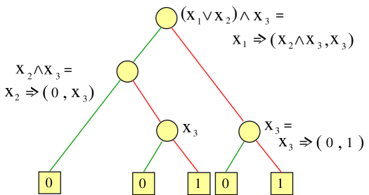
Figure 1: A decision tree for $(x_{1}\vee x_{2})\wedge x_{3}$.

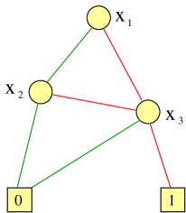
Figure 2: A BDD for $(x_{1}\vee x_{2})\wedge x_{3}$.

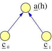
Figure 3: If-then-else node.

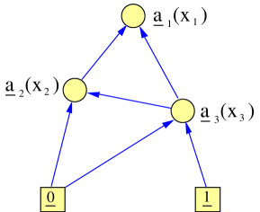
Figure 4: A Bayesian net for $(x_{1}\vee x_{2})\wedge x_{3}$.

In the field of Bayesian nets, one can define an if-then-else node. See Fig.3. The node is labelled by a random variable $\underline{a}(h)$ which depends on a Boolean parameter $h$. The node has two possible states, $0$ and $1$. The transition probability associated with node $\underline{a}(h)$ is given by

$$P\{\underline{a}(h)=a|c_{0},c_{1}\}=\delta^{a}_{h\Rightarrow(c_{0},c_{1})}\;,$$ (7)

for all $h,a,c_{0},c_{1}\in Bool$. This transition probability can be expressed in table form as follows. For $h=0$, one has

$$P\{\underline{a}(0)=a|c_{0},c_{1}\}=\left\{\begin{array}[]{cc}&(c_{0},c_{1})\rightarrow\\ \begin{array}[]{c}a\\ \downarrow\end{array}&\begin{array}[]{c|cccc}&00&01&10&11\\ \hline\cr 0&1&1&0&0\\ 1&0&0&1&1\end{array}\\ \end{array}\right.\;,$$ (8)

and for $h=1$,

$$P\{\underline{a}(1)=a|c_{0},c_{1}\}=\left\{\begin{array}[]{cc}&(c_{0},c_{1})\rightarrow\\ \begin{array}[]{c}a\\ \downarrow\end{array}&\begin{array}[]{c|cccc}&00&01&10&11\\ \hline\cr 0&1&0&1&0\\ 1&0&1&0&1\end{array}\\ \end{array}\right.\;.$$ (9)

Note that these probabilities are all deterministic, meaning that they are all either 0 or 1, none is a fraction.

The BDD of Fig.2 is equivalent to the Bayesian Net of Fig.4. Note that these two dags are identical. In the Bayesian net of Fig.4, all nodes are if-then-else nodes except for the square ones. Square nodes have two states, 0 and 1. Node $\underline{0}$ (resp., node $\underline{1}$) is in state 0 (resp., state 1) with probability 1, and in the opposite state with probability 0.

It is now clear that BDDs are just a special kind of Bayesian Net.

	BDD	Bayesian Net
number of states	2	arbitrary
of a node
number of arrows	2 if round node,	arbitrary
entering a node	0 if square node
transition probabilities	deterministic	arbitrary
for a node
number of nodes	1	arbitrary
at top of graph
number of nodes	2	arbitrary
at bottom of graph

References

-
[1]
The field of BDDs started with the following paper:
“Graph Based Algorithms for Boolean Function Manipulation”,
by Randal E. Bryant, IEEE Trans. on Computers, 8(C-35)677, 1986.
This paper is available at Bryant’s website:
http://www-2.cs.cmu.edu/~bryant/ -
[2]
“An Introduction to Binary Decision Diagrams”, by Henrik Reif Andersen.
Available at Andersen’s website:
http://www.itu.dk/people/hra/ -
[3]
For an introduction to Bayesian Nets, see, for example,
this web site:
http://www.cs.berkeley.edu/~murphyk/Bayes/bayes.html