Nonclassical effects in cold trapped ions inside a cavity

Abstract

We investigate the dynamics of a cold trapped ion coupled to the quantized field inside a high-finesse cavity, considering exact resonance between the ionic internal levels and the field (carrier transition). We derive an intensity-dependent hamiltonian in which terms proportional to the square of the Lamb-Dicke parameter ($\eta$) are retained. We show that different nonclassical effects arise in the dynamics of the ionic population inversion, depending on the initial states of the vibrational motion/field and on the values of $\eta$.

I Introduction

The manipulation of simple quantum systems such as trapped ions wine98 has opened new possibilities regarding not only the investigation of foundations of quantum mechanics, but also applications on quantum information. In such a system, internal degrees of freedom of an atomic ion may be coupled to the electromagnetic field as well as to the motional degrees of freedom of the ion’s center of mass. Under certain circumstances, in which full quantization of the three sub-systems becomes necessary, we have an interesting combination of two bosonic systems coupled to a spin like system. A possibility is to place the ion inside a high finesse cavity in such a way that the quantized field gets coupled to the atom. A few papers discussing that arrangement may be found in the literature, e.g., the investigation of the influence of the field statistics on the ion dynamics zeng94 ; knight98 , the transfer of coherence between the motional states and the field parkins99 , a scheme for generation of matter-field Bell-type states ours01 , and even propositions of quantum logic gates gates . Several interaction hamiltonians analogue to the ones found in quantum optical resonance models may be constructed even in the case where the field is not quantized, but having the center-of-mass vibrational motion playing the role of the field. For instance, if we consider a two-level atom having atomic transition $\omega_{0}$ and center-of-mass oscillation frequency of $\nu$ in interaction with a laser of frequency $\omega_{L}$, if $\omega_{L}-\omega_{0}=-\nu$ (laser tuned to the first red sideband), it results an interaction hamiltonian of the Jaynes-Cummings type

$$\hat{H}_{i}=i\hbar\Omega(\sigma_{+}\hat{a}-\sigma_{-}\hat{a}^{\dagger}).$$ (1)

If $\omega_{L}-\omega_{0}=\nu$ (laser tuned to the first blue sideband), the resulting hamiltonian is an “anti-Jaynes-Cummings” type, or

$$\hat{H}_{i}=i\hbar\Omega(\sigma_{+}\hat{a}^{\dagger}-\sigma_{-}\hat{a}).$$ (2)

Note that here the bosonic operators, $\hat{a}^{\dagger},\hat{a}$, are relative to the center-of-mass oscillation motion. The ion itself is considered to be confined in a region much smaller than the laser light wavelength (Lamb-Dicke regime). Other forms of interaction hamiltonians may be constructed in a similar way vogel95 ; gerry97 .

In this paper we explore further the consequences of having the trapped ion in interaction with a quantized field. We show that under certain conditions, the quantum nature of the field is able to induce intensity-dependent effects in the trapped ion dynamics, somehow analogue to models in cavity quantum electrodynamics buck81 ; ours98 . We shall remark that here we derive a hamiltonian with an intensity-dependent coupling from a more general hamiltonian, which is different from the phenomenological approach discussed in buck81 ; ours98 .

II The model

We consider a single trapped ion, within a Paul trap, placed inside a high finesse cavity, and having a cavity mode coupled to the atomic ion. The vibrational motion is also coupled to the field as well as to the ionic internal degrees of freedom, in such a way that the hamiltonian will read knight98 ; ours01 .

$$\hat{H}=\hbar\nu\hat{a}^{\dagger}\hat{a}+\hbar\omega\hat{b}^{\dagger}\hat{b}+\hbar\frac{\omega_{0}}{2}\sigma_{z}+\hbar g(\sigma_{+}+\sigma_{-})(\hat{b}^{\dagger}+\hat{b})\cos\eta(\hat{a}^{\dagger}+\hat{a}),$$ (3)

where $\hat{a}^{\dagger}(\hat{a})$ denote the creation (annihilation) operators of the center-of-mass vibrational motion of the ion (frequency $\nu$), $\hat{b}^{\dagger}(\hat{b})$ are the creation (annihilation) operators of photons in the field mode (frequency $\omega$), $\omega_{0}$ is the atomic frequency transition, $g$ is the ion-field coupling constant, and $\eta=2\pi a_{0}/\lambda$ is the Lamb-Dicke parameter, being $a_{0}$ the amplitude of the harmonic motion and $\lambda$ the wavelength of light. Note that the ion’s position inside the cavity is different from the one considered in ours01 . Tipically the ion is well localized, confined in a region much smaller than light’s wavelenght, or $\eta\ll 1$ (Lamb-Dicke regime). Usually expansions up to the first order in $\eta$ are made in order simplify hamiltonians involving trapped ions, which results in Jaynes-Cummings like hamiltonians such as the ones in Eqs. (1) and (2). However, even for small values of the Lamb-Dicke parameter, we show that in the situation here discussed, an expansion up to second order in $\eta$ becomes necessary. Several interesting effects, such as long time scale revivals will depend on those terms, as we are going to show. We may expand the cosine in Eq. (3) and obtain

$$\cos\eta(\hat{a}^{\dagger}+\hat{a})\approx 1-\frac{\eta^{2}(1+2\hat{a}^{\dagger}\hat{a})}{2}-\frac{\eta^{2}(\hat{a}^{\dagger}{}^{2}+\hat{a}^{2})}{2}.$$ (4)

The interaction hamiltonian will become

$$\hat{H}_{i}=\hbar g\left[1-\frac{\eta^{2}(1+2\hat{a}^{\dagger}\hat{a})}{2}-\frac{\eta^{2}(\hat{a}^{\dagger}{}^{2}+\hat{a}^{2})}{2}\right](\sigma_{+}+\sigma_{-})(\hat{b}^{\dagger}+\hat{b}).$$ (5)

We may then rewrite the hamiltonian above in the interaction picture, in order to apply a rotating wave approximation. If we tune the light field so that it exactly matches the atomic transition, i.e., $\omega_{0}-\omega=0$ (carrier transition), and after discarding the rapidly oscillating terms, we obtain the following (interaction picture) interaction hamiltonian:

$$\hat{H}^{I}_{i}=\hbar g\left[1-\frac{\eta^{2}(1+2\hat{a}^{\dagger}\hat{a})}{2}\right](\sigma_{-}\hat{b}^{\dagger}+\sigma_{+}\hat{b}).$$ (6)

The resulting hamiltonian is alike a Jaynes-Cummings hamiltonian. It describes the annihilation of a photon and a simultaneous atomic excitation ($\hat{b}^{\dagger}$ and $\hat{b}$ are field operators), but having an effective coupling constant which depends on the excitation number ($\hat{a}^{\dagger}\hat{a}$) of the ionic oscillator. As we are going to show, this will bring interesting consequences on the ion’s center-of-mass dynamics. We would like to point out that we have retained terms of the order of $\eta^{2}$ in the co-sine expansion, which are much smaller than one. However, the product $\eta^{2}\langle\hat{a}^{\dagger}\hat{a}\rangle$ will not be negligible for a sufficiently large excitation number of the vibrational motion.

The evolution operator associated to the hamiltonian (6) is given by

$$\hat{U}(t)=\hat{C}_{m;n+1}|e\rangle\langle e|+\hat{C}_{m;n}|g\rangle\langle g|-i\hat{S}_{m;n+1}\hat{b}|e\rangle\langle g|-i\hat{b}^{\dagger}\hat{S}_{m;n+1}|g\rangle\langle e|,$$ (7)

where

$$\hat{C}_{m;n+1}=\cos\left(g\left[1-\eta^{2}(1+2\hat{m})/2\right]\sqrt{(\hat{n}+1)}\>t\right),$$ (8)

$$\hat{C}_{m;n}=\cos\left(g\left[1-\eta^{2}(1+2\hat{m})/2\right]\sqrt{\hat{n}}\>t\right),$$ (9)

and

$$\hat{S}_{m;n+1}=\frac{\sin\left(g\left[1-\eta^{2}(1+2\hat{m})/2\right]\sqrt{(\hat{n}+1)}\>t\right)}{\sqrt{(\hat{n}+1)}},$$ (10)

where we have used the notation $\hat{m}=\hat{a}^{\dagger}\hat{a}$ and $\hat{n}=\hat{b}^{\dagger}\hat{b}$.

We consider now the following (product) initial state

$$\hat{\rho}(0)=|e\rangle\langle e|\otimes\hat{\rho}_{f}(0)\otimes\hat{\rho}_{v}(0),$$ (11)

or ion’s internal levels prepared in the excited state $|e\rangle\langle e|$, the field prepared in a generic state $\hat{\rho}_{f}(0)$, and the ion’s vibrational center of mass motion prepared in a state $\hat{\rho}_{v}(0)$. Its time evolution, governed by the evolution operator (7) results, at a time $t$, in the following (joint) state,

$$\hat{\rho}(t) = \hat{C}_{m;n+1}\hat{\rho}_{f}(0)\hat{\rho}_{v}(0)\hat{C}_{m;n+1}|e\rangle\langle e|+\hat{b}^{\dagger}\hat{S}_{m;n+1}\hat{\rho}_{f}(0)\hat{\rho}_{v}(0)\hat{S}_{m;n+1}\hat{b}|g\rangle\langle g|$$ (12)

$$+ i\hat{C}_{m;n+1}\hat{\rho}_{f}(0)\hat{\rho}_{v}(0)\hat{S}_{m;n+1}\hat{b}|e\rangle\langle g|-i\hat{b}^{\dagger}\hat{S}_{m;n+1}\hat{\rho}_{f}(0)\hat{\rho}_{v}(0)\hat{C}_{m;n+1}|g\rangle\langle e|,$$

where the operators $\hat{C}$ and $\hat{S}$ are the ones in Eq. (8), (9) and (10) above.

The state in Eq. (12) is, in general, an entangled state involving the ion’s internal (electronic) degrees of freedom, the vibrational motion as well as the cavity field. We will now investigate the atomic population inversion considering simple initial states for the center-of-mass vibrational motion and the cavity field.

III Atomic dynamics

The (internal level) ionic dynamics will depend on the distributions of initial excitations of both the field and the center center-of-mass vibrational motion, given by $\langle n|\hat{\rho}_{f}(0)|n\rangle=\rho_{n,n}^{f}(0)$, $\langle m|\hat{\rho}_{v}(0)|m\rangle=\rho_{m,m}^{v}(0)$ respectively. For instance, the atomic population inversion may be written as

$$W(t)=Tr\left[\sigma_{z}\hat{\rho}(t)\right]=\sum_{n,m=0}^{\infty}\rho_{n,n}^{f}(0)\rho_{m,m}^{v}(0)\>\cos\left[2g\left(1-\eta^{2}(1+2m)/2\right)\sqrt{n+1}\>t\right].$$ (13)

Due to the different frequencies ($\nu=2g[1-\eta^{2}(1+2m)]\sqrt{n+1}$) in the co-sine argument, we expect different structures of beats in the inversion due to different preparations of the center-of-mass motion (index $m$, without a square root) and the field (index $n$, with $\sqrt{n+1}$). We immediately identify two well known particular cases - if the vibrational motion is prepared in a number state ($\rho^{v}_{m,m}(0)=\delta_{k,m}$), the atomic inversion in Eq. (13) will reduce to the characteristic pattern of the Jaynes-Cummings model - if otherwise the field is prepared in a number state ($\rho^{f}_{n,n}(0)=\delta_{l,n}$), we have a periodic behavior for the atomic inversion (no square root in the co-sine argument). This is shown in Fig. 1, where the field is initially in the vacuum state and the ion in a coherent state of the center-of-mass motion. The Lamb-Dicke parameter $\eta$ is typically less than unity, and the lowest order term in the expansion above, [see Eq.(4)] is of second order in $\eta$. Nevertheless, as we are going to show, interesting effects will arise if the term $\eta^{2}(1+2m)$ becomes large enough

We now consider both the center-of-mass motion and the field initially prepared in coherent states and the atom in the excited state $|e\rangle$. After performing the summation over $m$ in Eq.(13), we obtain the following expression

$$W(t)=\sum_{n=0}^{\infty}\rho_{n,n}^{f}(0)w_{n}(t),$$ (14)

with

$$w_{n}(t) = \exp\left\{-\overline{m}\left[1-\cos\left(2\eta^{2}\sqrt{n+1}\,gt\right)\right]\right\}$$ (15)

$$\times \cos\left\{2\left(1-\frac{\eta^{2}}{2}\right)\sqrt{n+1}\,gt-\overline{m}\,\sin\left[2\eta^{2}\sqrt{n+1}\,gt\right]\right\}.$$

The dynamics of the population inversion predicted by Eq. (13) may be interpreted in terms of two families of “revival” times. The revival times associated to the field ($t_{r}^{f}$), when terms $n$ and $n+1$ are in phase

$$gt_{r}^{f}\approx\frac{2k\pi\sqrt{\overline{n}}}{1-\frac{\eta^{2}(1+2\overline{m})}{2}};\ \ \ \ k=1,2,\ldots,$$ (16)

depend on $\overline{m}$, the mean excitation number of the center-of-mass motion, and on $\overline{n}$, the mean excitation number of the field. On the other hand, the revival times associated to the vibrational motion ($t_{r}^{v}$), when terms $m$ and $m+1$ are in phase, depend only on $\overline{n}$, the mean excitation number of the field, or

$$gt_{r}^{v}\approx\frac{k\pi}{\eta^{2}\sqrt{\overline{n}+1}};\ \ \ \ k=1,2,\ldots,$$ (17)

It is also possible to estimate collapse times in either case, or

$$gt_{c}^{f}\sim\frac{1}{1-\frac{\eta^{2}(1+2\overline{m})}{2}},$$ (18)

and

$$gt_{c}^{v}\sim\frac{1}{\eta^{2}\sqrt{\overline{m}(\overline{n}+1)}}.$$ (19)

We note that distinct patterns for the atomic inversion will arise depending on the values of $\eta^{2}$, $\overline{m}$ and $\overline{n}$, which are quantities determining the revival/collapse times. In order to appreciate those different situations, we show, in what follows, some plots of the atomic inversion for different excitations of the ionic motion and field as well as for different values of $\eta$.

In Fig. 2 we have a plot of the atomic inversion as a function of time, having $\eta=0.02$, $\overline{m}=4$ and $\overline{n}=25$. It is shown the usual pattern of collapses and revivals. In this case the relevant times are so that $gt_{c}^{f}\approx 1$ and $gt_{r}^{f}\approx 31$. For a larger Lamb-Dicke parameter, $\eta=0.04$, the oscillations in the atomic inversion are attenuated, as we see in Fig. 3. This means that one has to be careful while expanding over the parameter $\eta$, since in the model we are here discussing, terms of the order of $\eta^{2}$ have a significant influence on the system evolution. Another interesting behavior predicted by Eq. (13) is the phenomenon of “super-revivals” of the atomic inversion, or revivals taking place at long times. Those may occur in driven atoms sergio94 or in trapped ions under certain conditions ours99 . Our model also predicts “super revivals” if both the center-of-mass motion and the field are prepared in coherent states, as it is shown in Fig. 4 (same parameters as in Fig. 2). The “super revival” time in this case is given by $gt_{r}^{v}\approx 1540$, with a collapse time $gt_{c}^{v}\sim 245$. Still for long times, if $\eta=0.04$, as it is shown in Fig. 5, there will be changes in the “super revival” time, $gt_{r}^{v}\approx 385$ as well as in the collapse time, $gt_{c}^{v}\sim 61$. In this case the revival time for “ordinary revivals” is very close to the collapse time associated to the long time scale dynamics, so that the revivals themselves are attenuated (compare Fig. 2 with Fig. 3). Different patterns will occur for different values of $\overline{m}$ and $\overline{n}$. For instance, if $\overline{m}=25$, $\overline{n}=4$ and $\eta=0.2$, we have $gt_{r}^{v}\approx 48$ and $gt_{r}^{f}\approx 14$. In this case there is only one oscillation in the collapse region, as shown in Fig. 6. A different pattern for the oscillations occurs if the collapse time $gt_{c}^{v}\sim 24$ is slightly less than the revival time $gt_{r}^{f}\approx 26$ (see Fig. 7). The short time revivals are strongly suppressed, as we see in Fig. 7. We may compare the atomic inversion in Fig. 7 to the one in Fig. 2; in the latter case the collapse time is long enough to still allow revivals, while in the former one a shorter collapse time significantly reduces the amplitude of the revivals (at $gt_{r}^{f}\approx 26$). Apart from that, we also note a modulation in the oscillations, which is basically due to the combination of oscillations originated from the field and vibrational motion quanta distributions. As a final comment, we have that in the case of the periodic dynamics (Fig. 1), $gt_{r}^{f}=0$ and $gt_{r}^{v}\approx 1257$, which is in agreement with the revival times shown in Fig. 1. We would like also to point out that dissipation in the cavity and loss of coherence in the vibrational motion will certainly have a destructive action, and effects occurring at longer time scales may not be apparent. However, the atomic inversion is highly sensitive to the initial state preparation and the Lamb-Dicke parameter also for short times, and the observation of at least some of the effects above described might become possible with further improvements in the quality of cavities as well as in the control of trapped ions blatt .

IV Conclusion

We have investigated the dynamics of a single trapped ion enclosed in a cavity. We have found that, in the case of exact atom-field resonance (carrier transition), terms of the order of $\eta^{2}$ can make a significant contribution and should therefore be retained. This gives rise to a hamiltonian containing an intensity-dependent coupling. Besides, the quantum nature of the field plays an important role. We have shown that, the atomic inversion as a function of time may display different structures of beats depending on the initial preparation of the electromagnetic field and the ionic motion as well as on the Lamb-Dicke parameter $\eta$, and effects such as suppression/attenuation of the Rabi oscillations, long time scale revivals as well as a periodic dynamics may occur. Those interesting features may be understood in terms of the two collapse times and two revival times characteristic of the dynamics.

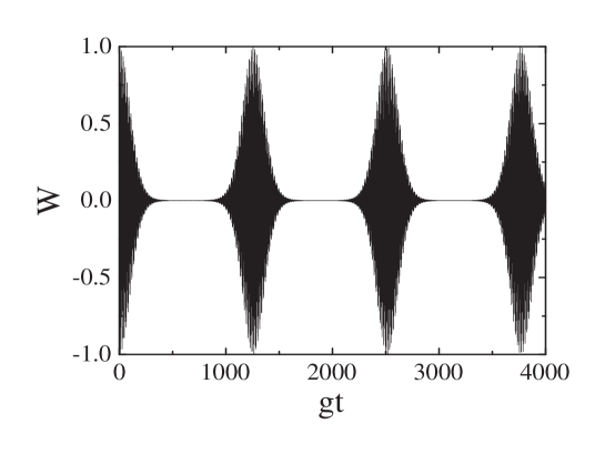
Figure 1: Atomic inversion as a function of the scaled time $gt$. The field is initially in the vacuum state, $\overline{n}=0$, and the vibrational motion in a coherent state with $\overline{m}=4$. The ion is prepared in its internal excited state, and $\eta=0.05$.

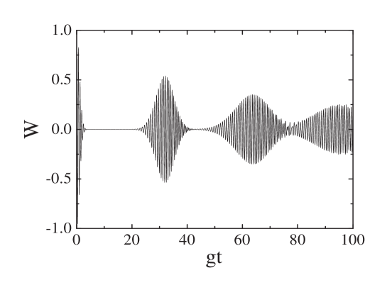
Figure 2: Atomic inversion as a function of the scaled time $gt$. The field is initially in a coherent state, $\overline{n}=25$, and the vibrational motion in a coherent state with $\overline{m}=4$. The ion is prepared in its internal excited state, and $\eta=0.02$.

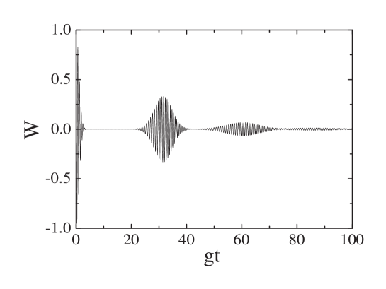
Figure 3: Atomic inversion as a function of the scaled time $gt$. The field is initially in a coherent state, $\overline{n}=25$, and the vibrational motion in a coherent state with $\overline{m}=4$. The ion is prepared in its internal excited state, and $\eta=0.04$.

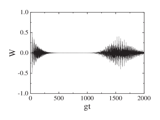
Figure 4: Atomic inversion as a function of the scaled time $gt$. The field is initially in a coherent state, $\overline{n}=25$, and the vibrational motion in a coherent state with $\overline{m}=4$. The ion is prepared in its internal excited state, and $\eta=0.02$.

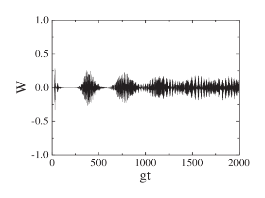
Figure 5: Atomic inversion as a function of the scaled time $gt$. The field is initially in a coherent state, $\overline{n}=25$, and the vibrational motion in a coherent state with $\overline{m}=4$. The ion is prepared in its internal excited state, and $\eta=0.04$.

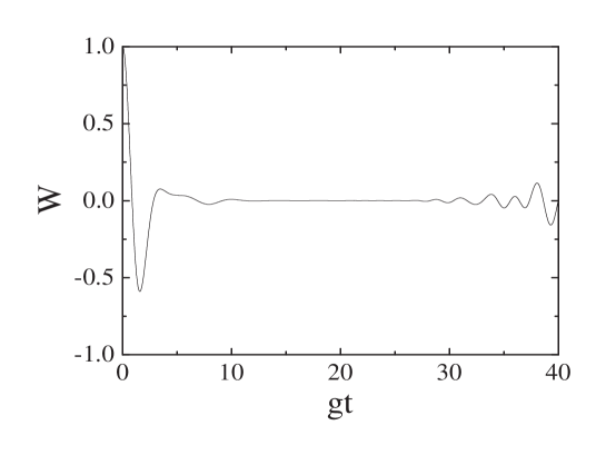
Figure 6: Atomic inversion as a function of the scaled time $gt$. The field is initially in a coherent state, $\overline{n}=1.69$, and the vibrational motion in a coherent state with $\overline{m}=10.24$. The ion is prepared in its internal excited state, and $\eta=0.2$.

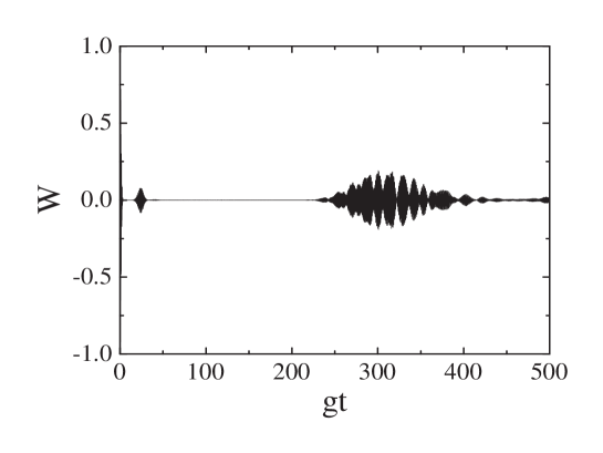
Figure 7: Atomic inversion as a function of the scaled time $gt$. The field is initially in a coherent state, $\overline{n}=16$, and the vibrational motion in a coherent state with $\overline{m}=16$. The ion is prepared in its internal excited state, and $\eta=0.05$.

- (1) D.J. Wineland, C. Monroe, W.M Itano, D. Leibfried, B.E. King, and D.M. Meekhof, NIST J. Res. 103, 259 (1998).
- (2) H. Zeng and F. Lin, Phys. Rev. A 50, R3589 (1994).
- (3) V. Bužek, G. Drobný, M.S. Kim, G. Adam, and P.L. Knight, Phys. Rev. A 56, 2352 (1998).
- (4) A.S. Parkins and H.J. Kimble, J. Opt. B: Quantum Semiclass Opt. 1, 496 (1999).
- (5) F.L. Semião, A. Vidiella-Barranco and J.A. Roversi, Phys. Rev. A 64, 024305 (2001).
- (6) F.L. Semião, A. Vidiella-Barranco and J.A. Roversi, Phys. Lett. A, 299, 423 (2002); E. Jané, M. B. Plenio, and D. Jonathan, Phys. Rev. A 65, 050302 (2002); M. Feng and X. Wang J. Opt. B: Quantum Semiclass. Opt. 4, 283 (2002); X.B. Zou, K. Pahlke, and W. Mathis, Phys. Rev. A 65, 064303 (2002); J. Pachos and H. Walther, quant-ph/0111088.
- (7) W. Vogel and R. L. de Matos Filho, Phys. Rev. A 52, 4214 (1995).
- (8) C.C. Gerry, Phys. Rev. A 55, 2478 (1997).
- (9) B. Buck and C.V. Sukumar, Phys. Lett. A, 81, 132 (1981).
- (10) Dagoberto S. Freitas and A. Vidiella-Barranco and J.A. Roversi, Phys. Lett. A, 249, 275 (1998).
- (11) S. M. Dutra and P. L. Knight and H. Moya-Cessa, Phys. Rev. A 49, 1993 (1994).
- (12) H. Moya-Cessa and A. Vidiella-Barranco and J. A. Roversi and D.S. Freitas and S.M. Dutra, Phys. Rev. A 59, 2518 (1999).
- (13) G.R. Guthörlein, M. Keller, K. Hayasaka, W. Lange, and H. Walther, Nature, 414 49 (2001); A. B. Mundt, A. Kreuter, C. Becher, D. Leibfried, J. Eschner, F. Schmidt-Kaler, and R. Blatt, Phys. Rev. Lett. 89, 103001 (2002); S. Gulde et al., to be published in Atomic Physics 18 (Proceedings of the ICAP 2002, also found in http://heart-c704.uibk.ac.at/papers.html).